

Significance
Active systems, from self-propelled colloids to animal swarms, can form complex dynamical patterns as their microscopic constituents exchange energy and momentum with the environment. Reflecting this complexity, continuum models for active matter typically possess many more parameters than those of classical fluids, like water. While much progress has been made in the qualitative understanding of active pattern formation, measuring the various hydrodynamic parameters of an active system still poses major challenges. Here, we present a broadly applicable computational framework that translates video data from self-propelled particle suspensions and fish swarms into continuum equations, yielding direct estimates for previously inaccessible hydrodynamic parameters and providing predictions that agree with recent experiments.
Keywords: active matter, sparse regression, coarse-graining, hydrodynamic equations
Abstract
Recent advances in high-resolution imaging techniques and particle-based simulation methods have enabled the precise microscopic characterization of collective dynamics in various biological and engineered active matter systems. In parallel, data-driven algorithms for learning interpretable continuum models have shown promising potential for the recovery of underlying partial differential equations (PDEs) from continuum simulation data. By contrast, learning macroscopic hydrodynamic equations for active matter directly from experiments or particle simulations remains a major challenge, especially when continuum models are not known a priori or analytic coarse graining fails, as often is the case for nondilute and heterogeneous systems. Here, we present a framework that leverages spectral basis representations and sparse regression algorithms to discover PDE models from microscopic simulation and experimental data, while incorporating the relevant physical symmetries. We illustrate the practical potential through a range of applications, from a chiral active particle model mimicking nonidentical swimming cells to recent microroller experiments and schooling fish. In all these cases, our scheme learns hydrodynamic equations that reproduce the self-organized collective dynamics observed in the simulations and experiments. This inference framework makes it possible to measure a large number of hydrodynamic parameters in parallel and directly from video data.
Natural and engineered active matter, from cells (1), tissues (2), and organisms (3) to self-propelled particle suspensions (4, 5) and autonomous robots (6–8), exhibits complex dynamics across a wide range of length and time scales. Predicting the collective self-organization and emergent behaviors of such systems requires extensions of traditional theories that go beyond conventional physical descriptions of nonliving matter (9–11). Due to the inherent complexity of active matter interactions in multicellular communities (12, 13) and organisms (14), or even nonequilibrium chemical (15) or colloidal (4, 5, 16) systems, it becomes increasingly difficult and inefficient for humans to formulate and quantitatively validate continuum theories from first principles. A key question is therefore whether one can utilize computing machines (17) to identify interpretable systems of equations that elucidate the mechanisms underlying collective active matter dynamics.
Enabled by recent major advances in microscopic imaging (12, 14, 18, 19) and agent-based computational modeling (20), active matter systems can now be observed and analyzed at unprecedented spatiotemporal (21–23) resolution. To infer interpretable predictive theories, the high-dimensional data recorded in experiments or simulations have to be compressed and translated into low-dimensional models. Such learned models must faithfully capture the macroscale dynamics of the relevant collective properties. Macroscale properties can be efficiently encoded through hydrodynamic variables, continuous fields that are linked to the symmetries and conservation laws of the underlying microscopic system (10, 11). Although much theoretical progress has been made in the field of dynamical systems learning over the last two decades (24–30), the inference of hydrodynamic models and their parameters from particle data has remained largely unsuccessful in practice, not least due to severe complications arising from measurement noise, inherent fluctuations, and self-organized scale-selection in active systems. Yet, extrapolating the current experimental revolution (4, 5, 12, 13, 18, 19), data-driven equation learning will become increasingly more important as simultaneous observations of physical, biological, and chemical properties of individual cells and other active units will become available in the near future (31, 32).
Learning algorithms for ordinary differential equations (ODEs) and partial differential equations (PDEs) have been proposed and demonstrated based on least-squares fitting (24, 25), symbolic regression (26, 27), and sparse regression (28, 29) combined with weak formulations (33–36), artificial neural networks (37–41), and stability selection (30, 42). These groundbreaking studies, however, focused primarily on synthetic data from a priori known continuum models, and recent coarse-graining applications have remained limited to ODEs (43) or one-dimensional (1D) PDEs (44, 45). By contrast, it is still an open challenge to infer higher-dimensional PDE models and measure hydrodynamic coefficients directly from microscopic active matter simulations or experiments.
Here, we present a comprehensive learning framework that takes microscopic particle data as input and proposes sparse interpretable hydrodynamic models as output (Fig. 1). We demonstrate its practical potential in applications to data from simulations of nonidentical active particles and recent experimental studies of microroller suspensions (4) as well as from schooling fish (46), for which the biophysical interactions are not exactly known. The learned hydrodynamic models replicate the emergent collective dynamics seen in the experimental videos, and their predictions agree with microroller experiments performed in different geometries. Furthermore, the linear hydrodynamic coefficients identified by the algorithm agree with independent estimates obtained by analytic coarse graining and active-sound spectroscopy (4). In addition, the framework identifies previously inaccessible nonlinear coefficients, providing data-informed closure relations for hydrodynamic models (10) of active matter when analytic coarse-graining procedures fail. From a broader theoretical perspective, the analysis below demonstrates how insights from analytic coarse-graining calculations and prior knowledge of conservation laws and broken symmetries can enhance the robustness of automated equation discovery from microscopic data. From a practical perspective, the algorithms and codes are directly applicable to imaging and tracking data generated in typical active matter experiments, offering a cost-efficient method for inferring hydrodynamic coefficients from videos.
Fig. 1.

Learning hydrodynamic models from particle simulations and experiments. (A) Inputs are time-series data for particle positions xi(t), particle orientations pi(t)=(cosθi, sinθi)⊤, etc., measured in simulations or experiments with microscale resolution (Active Particle Simulations). (B) Spatial kernel coarse graining of the discrete microscopic variables provides continuous hydrodynamic fields, such as the density ρ(t, x) or the polarization density p(t, x) (Hydrodynamic Fields). (C) Coarse-grained fields are sampled on a spatiotemporal grid and projected onto suitable spectral basis functions. Systematic spectral filtering (compression) ensures smoothly interpolated hydrodynamic fields, enabling efficient, and accurate computation of spatiotemporal derivatives (Spatiotemporal Representation and Differentiation). (D) Using these derivatives, a library of candidate terms Cl(ρ, p) and Cl(ρ, p) consistent with prior knowledge about conservation laws and broken symmetries is constructed. A sparse regression algorithm determines subsets of relevant phenomenological coefficients al and bl (Inference of Hydrodynamic Equations). The resulting hydrodynamic models are sparse and interpretable, and their predictions can be directly validated against analytic coarse-graining results (Validation and Discussion of Learned Models) or experiments (Learning from Experimental Data). Bottom: Snapshots illustrating the workflow for microscopic data generated from simulations of chiral active Brownian particles in Eq. 1.
1. Learning Framework
A. Active Particle Simulations.
To generate challenging test data for the learning algorithm, we simulated a 2D system of interacting self-propelled chiral particles (47–51) with broadly distributed propulsion and turning rate parameters. Microscopic models of this type are known to capture essential aspects of the experimentally observed self-organization of protein filaments (52, 53), bacterial swarms (21, 54, 55), and cell monolayers (56). In the simulations, a particle i with orientation pi = (cosθi, sinθi)⊤ moved and changed orientation according to the Brownian dynamics
| [1a] |
| [1b] |
where ηi(t) denotes orientational Gaussian white noise, with zero mean and ⟨ηi(t)ηj(t′)⟩=δijδ(t − t′), modulated by the rotational diffusion constant Dr. The parameter g > 0 determines the alignment interaction strength between particles i and j within a neighborhood 𝒩i of radius R. The self-propulsion speed vi ≥ 0 and orientational rotation frequency Ωi ≥ 0 were drawn from a joint distribution p(vi, Ωi) (SI Appendix, section A1). This heuristic distribution was chosen such that long-lived vortex states, similar to those observed in swimming sperm cell suspensions (57), formed spontaneously from arbitrary random initial conditions (Fig. 2A). Emerging vortices are left-handed for Ωi ≥ 0, and their typical size is ∼⟨vi⟩p/⟨Ωi⟩p, where ⟨ ⋅ ⟩p denotes an average over the parameter distribution p(vi, Ωi). We simulated Eq. 1 in a nondimensionalized form, choosing the interaction radius R as reference length and R/⟨vi⟩p as time scale. Accordingly, we set R = 1 and ⟨vi⟩p = 1 from now on. Simulations were performed for N = 12, 000 particles on a periodic domain of size 100 × 100 (Fig. 2A).
Fig. 2.

Learning mass conservation dynamics. (A) Top: Time evolution of positions and orientations of 12,000 particles following the dynamics in Eqs. 2a and 2b. Bottom: Coarse-grained density ρ (color code) and polarization field p (arrows). Starting from random initial conditions (t = 0), a long-lived vortex pattern with well-defined handedness emerges (t = 1, 250). Training data were randomly sampled from the time window t ∈ [40, 400], enclosed within the gray box. Domain size: 100 × 100. (B) Slices through the spatiotemporal power spectrum for different values of the Chebyshev polynomial order n ∈ {0, 300, 600}, corresponding to modes with increasing temporal frequencies. The rightmost panel depicts the total spatial spectral power ∑qSx; n, q of each Chebyshev mode n; see Eq. 3b. The slowly decaying long tail of fast modes indicates a regime in which fluctuations dominate over a smooth signal. The cutoff n0 = 600 removes these modes, in line with the goal to learn a hydrodynamic model for the slow long-wavelength modes. (C) Kymographs of the spectral derivatives ∂tρ and −∇⋅p at y = 50, obtained from the spectrally truncated data. (D) Mass conservation in the microscopic system restricts the physics-informed candidate library to terms that can be written as divergence of a vector field. (E) Learned phenomenological coefficients al of PDEs with increasing complexity (decreasing sparsity) (SI Appendix, section C). PDE 1 (◂) is given by ∂tρ = a1∇⋅p with a1 = −0.99. As PDE 1 is the sparsest PDE that agrees well with analytic coarse-graining results (Table 1), it is selected for the hydrodynamic model.
From a learning perspective, this model poses many of the typical challenges that one encounters when attempting to infer hydrodynamic equations from active matter experiments: spontaneous symmetry breaking and mesoscale pattern formation, microscopic parameter variability, noisy dynamics, anisotropic interactions, and so on. Indeed, similar to many experimental systems, it is not even clear a priori whether the heterogeneous active particle system described by Eq. 1 permits a description in terms of a sparse hydrodynamic continuum model, as the standard analytic coarse-graining procedure yields a physically unstable model (SI Appendix, section B1 and Fig. S5), reflecting the failure of ad hoc closure assumptions when parameters are broadly distributed. Below we will see that the learning framework is able to identify a set of hydrodynamic equations that replicate the key features of the particle simulations, including density patterns, vortex dynamics and scales, and spectral characteristics.
B. Hydrodynamic Fields.
Given particle-resolved data, hydrodynamic fields are obtained by coarse graining. A popular coarse-graining approach is based on convolution kernels (58, 59), weight functions that translate discrete fine-grained particle densities into continuous fields, analogous to the point-spread function of a microscope. For example, given the particle positions xi(t) and orientations pi(t), an associated particle number density field ρ(t, x) and polarization density field p(t, x) can be defined by
| [2a] |
| [2b] |
The symmetric kernel K(x) is centered at x = 0 and normalized, ∫d2x K(x)=1, so that the total number of particles is recovered from ∫d2x ρ(t, x)=N. Eqs. 2a and 2b generalize to higher tensorial density fields in a straightforward manner and can be readily adapted to accommodate different boundary conditions (SI Appendix, section A2).
We found that, in the context of hydrodynamic model learning, the coarse-graining Eqs. 2a and 2b with a Gaussian kernel K(x)∝exp[−|x|2/(2σ2)] present a useful preprocessing step that simplifies the use of fast transforms at later stages. The coarse-graining scale σ determines the spatial resolution of the hydrodynamic theory. In practice, σ must be chosen larger than the particles’ mean-free path length or interaction scale to ensure smoothness of the hydrodynamic fields but also smaller than the emergent collective structures. In accordance with these requirements, we fixed σ = 5 for the microscopic test data from Eq. 1 (Fig. 2A and SI Appendix, Fig. S13). Interestingly, measuring the spectral entropy as a function of σ for both simulated and experimental data showed that coarse-grained hydrodynamic fields typically maintain only about 1% of the spectral information contained in the fine-grained particle data (SI Appendix, section E and Figs. S13 and S14).
C. Spatiotemporal Representation and Differentiation.
A central challenge in PDE learning is the computation of spatial and temporal derivatives of the coarse-grained fields. Our framework exploits that hydrodynamic models aim to capture the long-wavelength dynamics of the slow collective modes (10). This fact allows us to project the coarse-grained fields on suitable basis functions that additionally enable sparse representations (high compression), fast transforms, and efficient differentiation. Here, we work with representations of the form
| [3a] |
| [3b] |
where Tn(t) denotes a degree-n Chebyshev polynomial of the first kind (60, 61), Fq(x)=exp(2πiq ⋅ x) is a Fourier mode with wave vector q = (qx, qy)⊤, and and are complex mode coefficients (Fig. 2B). Generally, the choice of the basis functions should be adapted to the spatiotemporal boundary conditions of the microscopic data (Learning from Experimental Data).
The spectral representation in Eq. 3 enables the efficient and accurate computation of space and time derivatives (62). Preprocessing via spatial coarse graining (Hydrodynamic Fields) ensures that the mode coefficients and decay fast for |q|≫1/(2πσ) (Fig. 2B, Left). If the asymptotic decay of the mode amplitudes with the temporal mode number n is at least exponential, then deterministic PDE descriptions are sufficient, whereas algebraically decaying temporal spectra indicate that stochastic PDEs may be required to capture essential aspects of the coarse-grained dynamics. For the simulated and experimental systems considered in this work, temporal spectra were found to decay exponentially (Fig. 2B) or superexponentially (SI Appendix, Fig. S17), suggesting the existence of deterministic PDE-based hydrodynamic models. To infer such models from data, we focus on the slow hydrodynamic modes and filter out the fast modes with n > n0 by keeping only the dominant Chebyshev terms in Eq. 3. The cutoff value n0 can usually be directly inferred from a characteristic steep drop-off in the power spectrum of the data, which signals the transition to hydrodynamically irrelevant fast fluctuations (63) (Fig. 2B, Right). Choosing n0 according to this criterion yields accurate, spatiotemporally consistent derivatives as illustrated for the kymographs of the derivative fields ∂tρ and −∇⋅p, which are essential to capture mass conservation. More generally, combining kernel-based and spectral coarse graining also mitigates measurement noise, enabling a direct application to experimental data (Learning from Experimental Data).
D. Inference of Hydrodynamic Equations.
To infer hydrodynamic models that are consistent with the coarse-grained projected fields from Eq. 3, we build on a recently proposed sparse regression framework (28, 29). The specific aim is to determine sparse PDEs for the density and polarization dynamics of the form
| [4a] |
| [4b] |
Additional dynamic equations and libraries can be added to Eq. 4 if, for example, higher-rank orientational order-parameter fields (such as a Q-tensor field describing spatiotemporal nematic order; SI Appendix, section B2) are dynamically relevant and can be extracted from microscopic data. For self-propelled polar systems, the relaxation of higher-rank hydrodynamic fields is typically fast compared to the relaxation of the polar orientation field (64). In this case, higher-rank tensorial fields are dynamically less relevant and can often be approximated by lower-rank fields and their derivatives through theoretically or empirically motivated closure relations (9, 10, 48). Accordingly, for the active particle data considered here, ρ and p present a natural choice for the hydrodynamic variables in a minimal mean-field description. This rationale is supported by generic analytic coarse-graining arguments (SI Appendix, section B), which also suggest first-order-in-time dynamics as described by Eq. 4.
The candidate library terms {Cl(ρ,p)} and {Cl(ρ,p)} are functions of the fields and their derivatives, which can be directly evaluated using spectral representation Eq. 3 at various sample points. Eq. 4 thus define a linear system for the phenomenological coefficients al and bl, and the objective is to find sparse solutions such that the resulting hydrodynamic model recapitulates the collective particle dynamics.
Hydrodynamic models for both equilibrium and nonequilibrium systems must respect the symmetries of the underlying microscopic dynamics. This requirement is a natural extension (65) of Landau-type theories for equilibrium systems, which derive hydrodynamic models from gradients of free energies that have to respect the symmetries of the underlying microscopic dynamics. However, continuum theories of nonequilibrium systems can have additional terms that are not functional derivatives of potentials, requiring more general libraries to perform model inference. Notwithstanding, prior knowledge of symmetries can greatly accelerate the inference process by placing constraints on the continuum model parameters. For example, the learning ansatz Eq. 4b already assumes global rotational invariance by using identical coefficients bl for the x and y components of the polarization field equations. Generally, coordinate independence of hydrodynamic models demands that the dynamical fields and the library functions Cl, Cl, etc., have the correct scalar, vectorial, or tensorial transformation properties. This fact imposes stringent constraints on permissible libraries, as do microscopic conservation laws, such as particle number conservation.
D.1. Symmetries and conservation laws: Generating a physics-informed candidate library.
Whenever prior knowledge about (broken) symmetries and conservation laws is available, it should inform the candidate library construction to ensure that the PDE learning is performed within a properly constrained model space. A useful constraint that holds in many experimental active matter systems as well as in the microscopic model in Eq. 1 arises from particle number conservation. To impose a corresponding mass conservation in the learned hydrodynamic models, we can restrict the scalar library terms Cl(ρ, p) in Eq. 4a to expressions that can be written as the divergence of a vector field. In this case, each term represents a different contribution to an overall mass flux, and mass conservation holds by construction for any model that will be learned. For the application considered in this work, we included fluxes up to first order in derivatives and third order in the fields (Fig. 2D). If required, such an approach can easily be generalized to other conservation laws, which then require libraries to be constructed exclusively from divergences of suitable tensors.
The active particle model in Eq. 1 describes a chiral dynamical system with intrinsic microscopic rotation rates Ωi ≥ 0. The space of valid hydrodynamic models therefore includes PDEs in which the mirror symmetry is explicitly broken. Formally, this implies that the Levi-Civita symbol ϵij can be used to generate a pseudovector p⊥ := ϵ⊤ ⋅ p = ( − py, px)⊤ that has to be included in the construction of the candidate libraries {Cl(ρ,p)} and {Cl(ρ,p)}. The vectorial library {Cl(ρ,p)} for the chiral polarization dynamics, Eq. 4b, cannot be constrained further by symmetries or conservation laws. Mechanical substrate interactions with the environment as invoked by the microscopic model in Eq. 1 and present in many active matter experiments explicitly break Galilean invariance, leading to external forces and torques whose form is not known a priori. We therefore included in Eq. 4b also vector fields that cannot be written as a divergence, such as p⊥, ρp or (p ⋅ ∇)p, in our candidate library {Cl(ρ,p)}.
In general, higher-order terms can be systematically constructed from the basic set of available fields and operators ℬ = {ρ, p, p⊥, ∇}. We illustrate the general procedure for an example library containing terms up to linear order in ρ and up to cubic order of the other terms in ℬ. The first step is to write the list of distinct rank-2 tensors
| [5] |
where s ∈ {1,ρ,∇⋅p,∇⋅p⊥} represents one of the linearly independent scalars that can be formed from elements in ℬ. From any tensor and its transpose, we can then generate vectorial terms Cl by forming scalar products with the elements in ℬ. In particular, terms yield possible contributions from internal stresses and torques due to alignment interactions, while and correspond to substrate-dependent interactions. Note that we omitted ϵ from the set 𝒮, as it yields only one additional linearly independent term ∼∇⊥ρ that can be excluded for the microscopic dynamics in Eq. 1a on the basis of generic coarse-graining arguments (SI Appendix, section B2).
For pattern-forming systems with emergent length scale selection, the library should be extended to include Swift–Hohenberg-type (66) terms Δ2p, Δ2p⊥, etc. (67, 68). Such terms can stabilize small-wavelength modes and, combined with Δp and Δp⊥, can give rise to patterns of well-defined length (66). The final 19-term library with linearly independent terms (SI Appendix, section A5) used to learn the polarization dynamics for the chiral particle model from Eq. 1 is summarized in Fig. 3C.
Fig. 3.

Learning polarization dynamics. (A) Same particle dynamics as in Fig. 2A for visual reference. (B) Top: Coarse-grained density and polarization field as in Fig. 2A. Bottom: Magnitude |p| of the coarse-grained polarization field. Emerging vortices (t=400, 1,250) appear as ring-like patterns in |p|. Training data were randomly sampled from the time window t ∈ [40, 400], enclosed within the gray box. (C) Physics-informed candidate library (with b1 = −Dr) including terms constructed from p⊥ = ( − py, px)⊤, which are allowed due to the chirality of the microscopic system. (D) Learned phenomenological coefficients bl of PDEs with increasing complexity (SI Appendix, section C). For all PDEs, learned coefficients of the linear terms p⊥ and ∇ρ compare well with analytic predictions (Table 1 and SI Appendix, section B2). (E) Simulation of the final hydrodynamic model (PDE 8 for the polarization dynamics and PDE 1 in Fig. 2E for the density dynamics). Starting from random initial conditions (t = 0), long-lived vortex states emerge on a similar time scale, with similar spatial patterns, and with comparable density and polarization amplitudes as in the coarse-grained microscopic model data (B). Hydrodynamic models with PDEs sparser than PDE 8 do not form stable vortex patterns.
D.2. Sparse model learning.
To determine the hydrodynamic parameters al and bl in Eq. 4, we randomly sampled the coarse-grained fields ρ(t, x) and p(t, x) and their derivatives at ∼106 space-time points within a predetermined learning interval (SI Appendix, section A). Generally, the success or failure of hydrodynamic model learning depends crucially on the choice of an appropriate space-time sampling interval. As a guiding principle, learning should be performed during the relaxation stage, when both time and space derivatives show the most substantial variation.
Evaluating Eqs. 4a and b at all sample points yields linear systems of the form , where the vector Ut contains the time derivatives (SI Appendix, section A3). The columns of the matrix hold the numerical values of the library terms Cl(ρ, p) and Cl(ρ, p) computed from the spectral representations in Eq. 3. The aim is to infer a parsimonious model so that the vector ξ containing the hydrodynamic parameters al or bl is sparse. In this case, the corresponding PDE contains only a subset of the library terms, and we refer to the total number of terms in a PDE as its complexity.
To estimate sparse parameters ξ, we used the previously proposed sequentially thresholded least-squares (STLSQ) algorithm from SINDy (28). STLSQ first finds the least-squares estimate . Subsequently, sparsity of is imposed by iteratively setting coefficients below a thresholding hyperparameter τ to zero. By construction, this regression uses data only from the bulk of the domain and therefore does not require information about boundary conditions. Adopting a stability selection approach (30, 42, 69, 70) in which τ is systematically varied over a regularization path [τmax, τmin] (SI Appendix, section A3), we obtain candidate PDEs of increasing complexity (Figs. 2E and 3D) whose predictions need to be validated against the phenomenology of the input data.
D.3. Performance improvements and pitfalls.
Sparse regression-based learning becomes more efficient and robust if known symmetries or other available information can be used to reduce the number of undetermined parameters al and bl in Eq. 4. Equally helpful and important is prior knowledge of the relevant time and length scales. The coarse-grained field data need to be sampled across spatiotemporal scales that contain sufficient dynamical information; oversampling in a steady-state typically prevents algorithms from learning terms relevant to the relaxation dynamics. Systems exhibiting slow diffusion time scales can pose additional challenges. For example, generic analytic coarse graining (SI Appendix, section B1) shows that additive rotational noise as in Eq. 1b implies the linear term −Drp in the polarization dynamics in Eq. 4b. If the diffusive time scale 1/Dr approaches or exceeds the duration of the sampling time interval, then the learned PDEs may not properly capture the relaxation dynamics of the polarization field. From a practical perspective, this is not a prohibitive obstacle, as the rotational diffusion coefficient Dr can be often measured independently from isolated single-particle trajectories (71). In this case, fixing −Drp in Eq. 4b and performing the regression over the remaining parameters produced satisfactory learning results (Fig. 3, where 1/Dr ∼ 100 is comparable to the length of the learning interval t ∈ [40, 400]).
E. Validation and Discussion of Learned Models.
The STLSQ algorithm with stability selection proposes PDEs of increasing complexity—The final learning step is to identify the sparsest acceptable hydrodynamic model among these (Fig. 1). This can be achieved by simulating all the candidate PDEs (SI Appendix, section A6) and comparing their predictions against the original data and, if available, against analytic coarse-graining results (SI Appendix, section B).
For the microscopic particle model from Eq. 1, the sparsest learned PDE for the particle number density is ∂tρ = a1∇⋅p (Fig. 2E); this mass conservation equation is also predicted by analytic coarse graining (SI Appendix, section B). The learned coefficient a1 = −0.99 implies an effective number density flux −a1p ≈ p, which agrees very well with the analytic prediction ⟨vi⟩pp = p. Additional coefficients appearing in more complex models proposed by the algorithm are at least one order of magnitude smaller than a1 (Fig. 2E). Hence, as part of a hydrodynamic description of the microscopic system in Eq. 1, we adopt the minimal density dynamics ∂tρ = a1∇⋅p from now on.
The sparsest learned PDE for the dynamics of the polarization field p contains only three terms. However, together with the density dynamics, the resulting hydrodynamic models are either unstable or do not lead to the formation of vortex patterns. Our simulations showed that a certain level of model complexity is required to reproduce the dynamics observed in the test data. In particular, there exists a unique sparsest model (PDE 8 in Fig. 3D) for which long-lived vortex states emerge from random initial conditions. The resulting hydrodynamic model exhibits density and polarization patterns matching those observed in the original particle system (Fig. 3A, B, and E and SI Appendix, Movie S1), which also form on a similar time scale. Furthermore, the learned coefficients of the linear terms ∼p⊥ and ∼∇ρ agree well with the analytic predictions (Table 1 and SI Appendix, section B2). A direct comparison of temporal and spatial spectra from simulations of the learned hydrodynamic model with the coarse-grained original data shows satisfactory agreement between the characteristic length and time scales seen in each dataset (SI Appendix, section D and Figs. S11 and S12). Furthermore, density profiles, vortex sizes, and the disordered nature of emergent vortex patterns are also consistent between the coarse-grained particle data and the learned model (SI Appendix, Fig. S10), confirming that the learned model captures key features of the collective hydrodynamic modes.
Table 1.
Parameters of the hydrodynamic model learned for the microscopic dynamics in Eq. 1 and values predicted by analytic coarse graining (SI Appendix, section B2)

|
The individual terms appearing in the learned hydrodynamic equations identify specific physical mechanisms that contribute to emergent pattern formation. The linear contributions are directly interpretable based on generic analytic coarse-graining arguments (SI Appendix, section B): The term b1p with b1 < 0 corresponds to the lowest-order mean-field contribution of rotational diffusion that suppresses orientational order at long times. The chiral term b3p⊥ with b3 > 0 drives counterclockwise rotations of the local polar field since ∂tp = b3p⊥ is solved by the rotating vector field p = (cosb3t, sinb3t). This term represents the lowest-order chiral mean-field contribution to the dynamics and is a direct consequence of the active rotations ∼Ωi of single particles in Eq. 1b. The term b7∇ρ with b7 < 0 comes from an effective extensile isotropic stress σ ∼ −b7ρ𝕀 that arises entropically in systems with moving polar particles (SI Appendix, section B2). The nonlinear ρp and |p|2p terms represent density-dependent polar alignment interactions, similar to ferromagnetic interactions in spin systems. Other higher-order and nonlinear terms can be identified as contributions from an effective closure relation, capturing the interplay between polar and nematic order in the particle system, or from effects of the microscopic parameter variability. (A detailed discussion is provided in SI Appendix, section B3.) We emphasize that, for the microscopic model in Eq. 1, standard methods for analytically deriving coarse-grained hydrodynamic equations (10, 48, 49, 55, 64, 72, 73) predict coefficients for nonlinear terms that are quantitatively different from those in our learned equations (SI Appendix, Table SI). Even more critically, the analytically derived model does not correctly capture vortex pattern formation, instead exhibiting locally diverging mass and polarization densities that render simulations unstable (SI Appendix, Fig. S5). By contrast, the learned hydrodynamic model is numerically stable and correctly reproduces the vortex formation seen in the particle simulations.
As the learning algorithm used coarse-grained field data only in the time interval t ∈ [40, 400], simulation results for t > 400 represent predictions of the learned hydrodynamic model (Fig. 3E). The close agreement between original data and the model simulations (Fig. 3 B and E) shows that the inference framework has succeeded in learning a previously unknown hydrodynamic description for a chiral polar active particle system with broadly distributed microscopic parameters.
2. Learning from Experimental Data
The inference framework can be readily applied to experimental data. We illustrate this by learning a hydrodynamic model directly from a video recorded in a recent study (4) of driven colloidal suspensions (Fig. 4A). In these experiments, an electrohydrodynamic instability enables micron-sized particles to self-propel with speeds up to a few millimeters per second across a surface. The rich collective dynamics of these so-called Quincke rollers (4, 74) provides a striking experimental realization of self-organization in active polar particle systems (10, 75, 76).
Fig. 4.

Learning from active polar particle experiments. (A) Snapshot of particle positions and velocity components of ∼2,200 spontaneously moving Quincke rollers in a microfluidic channel (4). (Scale bar, 200 µm.) (B) Coarse-grained density field ρ(t, x), expressed as the fraction of area occupied by the rollers with diameter Dc = 4.8 µm, and components vx(t, x) and vy(t, x) of the coarse-grained velocity field (σ = 45 µm). 5 × 10⁵ randomly sampled data points from ∼580 such snapshots over a time duration of 1.4 s were used for the learning algorithm. (C) Physics-informed candidate libraries for the density and velocity dynamics, and , respectively, Eq. 6b. These are the same libraries as shown in Figs. 2E and 3D but without the chiral terms and replacing p → v. (D) Learned phenomenological coefficients cl and dl of the four sparsest PDEs for the density (Left) and velocity (Right) dynamics. The coefficients are nondimensionalized with length scale σ and time scale σ/v0, where v0 = 1.2 mm s−1 is the average roller speed. PDE 1 for density dynamics corresponds to ∂tρ = c3∇⋅(ρv) with c3 ≃ −0.95. PDE 2 for the velocity dynamics is shown in Eq. 7b. Learned coefficients compare well with the values reported in ref. 4 (Table 2). (E) Simulation snapshot at t = 1.8 s of the learned hydrodynamic model (PDEs marked by ◂ in (D) in a doubly periodic domain. Spontaneous flow emerges from random initial conditions and exhibits density and velocity fluctuations that show similar spatial patterns and amplitudes as seen in the experiments (A). (F) Simulation snapshots at t = 18.5 s of the same hydrodynamic model as in (E) on a square domain with reflective boundary conditions. The model predicts the emergence of a vortex-like flow permeated by density shock waves. This prediction agrees qualitatively with experimental observations (Rightmost) of Quincke rollers in a 5 mm× 5 mm confinement with average density ρ0 ≈ 0.1 (Image credits: Alexandre Morin, Delphine Geyer, and Denis Bartolo). (Scale bars, 200 µm (simulation) and 1 mm (experiment).)
A. Coarse Graining and Spectral Representation of Experimental Data.
To gather dynamic particle data from experiments, we extracted particle positions xi(t) from the SI Appendix, Movie S2 in ref. 4, with particle velocities vi(t)=dxi/dt replacing the particle orientations pi(t) from before. This dataset captures a weakly compressible suspension of Quincke rollers in a part of a racetrack-shaped channel (Fig. 4A). We then applied the kernel coarse graining in Eq. 2 with σ = 45 μm, SI Appendix, Fig. S14 to obtain the density field ρ and the velocity field v = p/ρ. Accounting for the nonperiodicity of the data, ρ and v were projected on a Chebyshev polynomial basis, Eq. 3, in time and space (Fig. 4B). Filtering out nonhydrodynamic fast modes with temporal mode numbers n > n0, we found that the final learning results were robust for a large range of cutoff modes n0 (SI Appendix, section C).
B. Physics-Informed Library.
The goal is to learn a hydrodynamic model of the form
| [6a] |
| [6b] |
where and denote library terms with coefficients cl and dl, respectively. The experimental Quincke roller system shares several key features with the particle model in Eq. 1, so the construction of the candidate libraries and follows similar principles (Fig. 4C). Conservation of the particle number implies that can be written as divergences of vector fields. However, rollers do not explicitly break mirror symmetry, so chiral terms can be dropped from the library, leaving the candidate terms shown in Fig. 4C.
C. Learned Hydrodynamic Equations and Validation.
The sparse regression algorithm proposed a hierarchy of hydrodynamic models with increasing complexity (Fig. 4D). The sparsest learned model that recapitulates the experimental observations is given by
| [7a] |
| [7b] |
Notably, Eqs. 7a and 7b contain all the relevant terms to describe the propagation of underdamped sound waves, a counterintuitive, but characteristic feature of overdamped active polar particle systems (4).
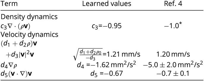
Although the finite experimental observation window and imperfect particle tracking was expected to limit the accuracy of the learned models, the learned coefficient values agree well with corresponding parameters estimated in ref. 4 by fitting a linearized Toner-Tu model to the experimental data (Table 2). The coefficient c3 ≃ −0.95 in the mass conservation equation is close to the theoretically expected value −1. The learned coefficient d4 in the velocity Eq. 7b is of similar magnitude but slightly less negative than the dispersion-based estimate in ref. 4. The learned coefficients d1, d2, and d3 are described in SI Appendix, Table SVI. Despite being inferred from a single video, these parameters yield a remarkably accurate prediction for the typical roller speed as a function of the area fraction ρ0 (SI Appendix, Fig. S4 in ref. 4 and Fig. 5). Similarly, the learned coefficient d5 of the nonlinear advective term ∼(v ⋅ ∇)v is in close agreement with the value reported in ref. 4. Interestingly, d5 ≠ −1 reveals the broken Galilean invariance (9, 10) due to fluid-mediated roller–substrate interaction, a key physical aspect of the experimental system that is robustly discovered by the hydrodynamic model learning framework.
Table 2.
Parameters of the learned hydrodynamic model for the Quincke roller system are close to values expected from analytic coarse graining (*) and reported in ref. 4 for experiments performed at mean area fraction ρ0≈0.11
|
Fig. 5.

The learned model accurately predicts collective Quincke roller speeds v0 at different average area fractions ρ0. Although Eq. 7 was learned from a single experiment (SI Appendix, Movie S2 in ref. 4) at fixed average area fraction ρ0 = 0.11 (filled black circle), the model prediction (solid line) with inferred parameters d1, d2, d3 (SI Appendix, Table SVI), agrees well the experimentally measured speed values (red symbols) reported in SI Appendix, Fig. S4 of ref. 4.
To validate the learned hydrodynamic model, we simulated Eq. 7 on a periodic domain comparable to the experimental observation window (Fig. 4E and SI Appendix, section A6). Starting from random initial conditions, spontaneously flowing states emerge (SI Appendix, Movie S2), even though the spontaneous onset of particle flow is not a part of the experimental data from which the model was learned. The emergent density and flow patterns are quantitatively similar to the experimentally observed ones. In particular, the learned model predicts the formation of transverse velocity bands as seen in the experiments (Fig. 4B and E).
D. Predicting Collective Roller Dynamics in Confinement.
Useful models must be able to make predictions for a variety of experimental conditions. At minimum, if a learned hydrodynamic model captures the most relevant physics of an active system, then it should remain valid in different geometries and boundary conditions. To confirm this for the Quincke system, we simulated Eq. 7 on a square domain using no-flux and shear-free boundary conditions (SI Appendix, section A6). Starting from random initial conditions, our learned model predicts the formation of a vortex-like flow, permeated by four interwoven density shock waves, which arise from reflections at the boundary (Fig. 4F, Left and SI Appendix, Movie S3). Remarkably, this behavior has indeed been observed in experiments (74) in which Quincke rollers were confined within a square domain (Fig. 4F, Right). These results demonstrate the practical potential of automated model learning for complex active matter systems. As an additional demonstration, we present in SI Appendix, section F an application of the above learning framework to recent fish schooling experiments (46). In this case, the exact nature of the underlying fish–fish interactions, which likely involve both hydrodynamic (77, 78) and visual (79, 80) cues, is not exactly known. Interestingly, the inference algorithm identifies a sparse hydrodynamic model (SI Appendix, Table SVIII) that is structurally similar to the Quincke system (SI Appendix, Table SVI), despite a vast difference in scales.
E. Limitations and Outlook.
Any learning or inference framework is fundamentally limited by its underlying model space. In neural network (NN)-based machine learning schemes (39, 81–83), the NN architecture is prescribed by the human modeler, whose heuristically plausible yet ad hoc choices limit the range of predictable phenomena. In continuum dynamical systems inference (26, 28, 37, 84–86), as considered here, the spatiotemporal evolution of tensorial order-parameter fields is parameterized in terms of partial differential equations, and the range of predictable phenomena is limited by the choice of the library. Independent of whether one prefers NN-based, PDE-based, or other approaches, once the model space and its parameterization have been fixed, “learning” reduces to solving a high-dimensional (usually nonconvex) optimization problem. While NN models prioritize expressive power over interpretability, PDE-based models tend to be more easily interpretable and amenable to symmetry constraints, but their expressive power is inherently limited by the “domain knowledge” that informs library selection. An interesting approach toward reducing bias and increasing flexibility in model formulation are symbolic regression techniques (87–89) that could, in principle, discover novel classes of equations. Unfortunately, symbolic regression comes with high computational complexity, so that human-informed modeling frameworks will remain practically relevant in the physical and life sciences.
3. Discussion & Conclusions
Leveraging spectral representations of field observables and recent advances in the sparse PDE inference (28–30, 42), we have presented a PDE learning framework that robustly identifies hydrodynamic models for the self-organized dynamics of active matter systems. To illustrate its broad practical potential and applicability, we demonstrated the automated inference of interpretable hydrodynamic models from microscopic simulation data as well as from experimental video data for active and living systems (SI Appendix, section F). The underlying computational framework complements modern machine learning approaches, including model-free methods (90, 91) and others that leverage a priori known model structure to predict complex dynamics (39, 41, 59, 81), infer specific model parameters (92) or hidden fields (82), partially replace PDE models with suitably trained neural networks (40, 93), or use them for dimensionality reduction (94, 95).
Inferring sparse hydrodynamic models from coarse-grained active matter data also complements analytic coarse-graining techniques (10, 48, 49, 55, 64, 72, 73), which generally require ad hoc moment closures to truncate infinite hierarchies of coupled mode equations (SI Appendix, section B). Such closures typically neglect correlations and rely on approximations that may not be valid in heterogeneous interacting active matter systems. Automated learning of hydrodynamic equations instead yields data-informed closure relations, while simultaneously providing quantitative measurements of phenomenological coefficients (viscosities, elastic moduli, etc.) from video data (92). We have shown here that this data-driven approach yields well-defined, numerically stable continuum models in situations where analytic coarse-graining methods lead to hydrodynamic equations that do not reproduce the observed patterns and instead generate locally diverging density patterns (SI Appendix, Fig. S5).
Successful model learning requires both good data and a good library. Good data need to sample all dynamically relevant length and time scales (84). A good library is large enough to include all hydrodynamically relevant terms and small enough to enable robust sparse regression (30). Since the number of possible terms increases combinatorially with the number of fields and differential operators, library construction should be guided by prior knowledge of global, local, and explicitly broken symmetries. From a physics perspective, using symmetry considerations as a key guiding principle to construct phenomenological models naturally builds on Ginzburg–Landau-type approaches to nonequilibrium pattern formation (65, 96). Here, this approach enabled us to infer quantitative hydrodynamic models directly from particle data, consistent with symmetry constraints arising from the microscopic dynamics. From an algorithmic perspective, physics-informed libraries ensure properly constrained model search spaces, promising a more efficient sparse regression. Equally important is the use of suitable spectral field representations—without these, an accurate evaluation of the library terms seems nearly impossible even for very-high quality data.
In view of the above successful applications, which encompassed microscopic parameter variability, explicitly noisy particle dynamics, and measurement noise in experimental data, we expect that the computational framework presented here can be directly applied to a wide variety of passive and active matter systems. Specifically, the fish schooling (46) example (SI Appendix, section F) demonstrates that automated model inference can yield predictive continuum models even when the biophysical particle–particle interactions are highly complex (77–80) or not yet exactly known. The computational framework presented here can likely be enhanced by combining recent advances in sparse regression (42, 97) and weak formulations (35) with statistical information criteria (85) and cross-validation (98) for model selection. Furthermore, an extension to three dimensions is conceptually and computationally straightforward: Kernel-based coarse-graining, spectral data representation, the implementation of conservation laws through suitable restrictions of library terms, and the sparse regression scheme all extend naturally to higher dimensions in a parallelizable manner. Given the rapid progress in experimental imaging and tracking techniques (12, 14, 18, 19, 46), we anticipate that many previously intractable physical and biological systems will soon find interpretable quantitative continuum descriptions that may reveal novel ordering and self-organization principles.
Supplementary Material
Appendix 01 (PDF)
Supporting Video for Figs. 2 and 3 of the main text: Comparison of discrete particle dynamics and coarse-grained density and polarization fields from simulations of an active chiral Brownian particle model (Eqs. (1), main text; see SI Sec. A 1 for simulation details and model parameters) with simulations of the learned continuum model (see SI Secs. C and D for details of the continuum model and its parameters).
Supporting Video for Fig. 4A-E of the main text: Simulations of the learned continuum model for the experimental Quincke roller system in a channel geometry with periodic boundary conditions along the horizontal direction.
Supporting Video for Fig. 4F of the main text: Simulation of the learned continuum model for the Quincke roller system in a closed-square geometry recapitulates essential characteristics of the experimental observations.
Acknowledgments
We thank Keaton Burns for helpful advice on the continuum simulations, Henrik Ronellenfitsch for insightful discussions about learning methodologies, and the MIT SuperCloud for providing us access to HPC resources. We thank Tristan Walter and Iain Couzin for sharing and explaining the sunbleak data. This work was supported by a MathWorks Engineering Fellowship (R.S.), a Graduate Student Appreciation Fellowship from the MIT Mathematics Department (B.S.), a NSF Mathematical Sciences Postdoctoral Research Fellowship (DMS-2002103, G.P.T.C.), a Longterm Fellowship from the European Molecular Biology Organization (ALTF 528-2019, A.M.), a Postdoctoral Research Fellowship from the Deutsche Forschungsgemeinschaft (Project 431144836, A.M.), a Complex Systems Scholar Award from the James S. McDonnell Foundation (J.D.), NSF Award DMS-1952706 (J.D.), and the Robert E. Collins Distinguished Scholarship Fund (J.D.).
Author contributions
J.D. designed research; R.S., B.S., A.H., G.P.T.C., and A.M. performed research; and R.S., A.H., A.M., and J.D. wrote the paper.
Competing interests
The authors declare no competing interest.
Footnotes
This article is a PNAS Direct Submission.
Contributor Information
Alexander Mietke, Email: amietke@mit.edu.
Jörn Dunkel, Email: dunkel@mit.edu.
Data, Materials, and Software Availability
All study data are included in the article and/or SI Appendix. The codes and data required to generate Quincke Roller results are provided in this GitHub repository: https://github.com/rohitsupekar/learning-active-matter-equations. Due to size constraints, any other data are available from authors upon reasonable request.
Supporting Information
References
- 1.Tambe D. T., et al. , Collective cell guidance by cooperative intercellular forces. Nat. Mater. 10, 469–475 (2011). [DOI] [PMC free article] [PubMed] [Google Scholar]
- 2.Heisenberg C. P., Bellaïche Y., Forces in tissue morphogenesis and patterning. Cell 153, 948–962 (2013). [DOI] [PubMed] [Google Scholar]
- 3.Tennenbaum M., Liu Z., Hu D., Fernandez-Nieves A., Mechanics of fire ant aggregations. Nat. Mater. 15, 54–59 (2016). [DOI] [PubMed] [Google Scholar]
- 4.Geyer D., Morin A., Bartolo D., Sounds and hydrodynamics of polar active fluids. Nat. Mater. 17, 789–793 (2018). [DOI] [PubMed] [Google Scholar]
- 5.Soni V., et al. , The odd free surface flows of a colloidal chiral fluid. Nat. Phys. 15, 1188–1194 (2019). [Google Scholar]
- 6.Rubenstein M., Cornejo A., Nagpal R., Programmable self-assembly in a thousand-robot swarm. Science 345, 795–800 (2014). [DOI] [PubMed] [Google Scholar]
- 7.Nash L. M., et al. , Topological mechanics of gyroscopic metamaterials. Proc. Natl. Acad. Sci. U.S.A. 112, 14495–14500 (2015). [DOI] [PMC free article] [PubMed] [Google Scholar]
- 8.Savoie W., et al. , A robot made of robots: Emergent transport and control of a smarticle ensemble. Sci. Robot. 4, eaax4316 (2019). [DOI] [PubMed] [Google Scholar]
- 9.Toner J., Tu Y., Long-range order in a two-dimensional dynamical XY model: How birds fly together. Phys. Rev. Lett. 75, 4326–4329 (1995). [DOI] [PubMed] [Google Scholar]
- 10.Marchetti M. C., et al. , Hydrodynamics of soft active matter. Rev. Mod. Phys. 85, 1143–1189 (2013). [Google Scholar]
- 11.Jülicher F., Grill S. W., Salbreux G., Hydrodynamic theory of active matter. Rep. Prog. Phys. 81, 076601 (2018). [DOI] [PubMed] [Google Scholar]
- 12.Hartmann R., et al. , Emergence of three-dimensional order and structure in growing biofilms. Nat. Phys. 15, 251–256 (2019). [DOI] [PMC free article] [PubMed] [Google Scholar]
- 13.Li Y., et al. , Volumetric compression induces intracellular crowding to control intestinal organoid growth via wnt/β-catenin signaling. Cell Stem Cell 28, 63–78 (2021). [DOI] [PMC free article] [PubMed] [Google Scholar]
- 14.Shah G., et al. , Multi-scale imaging and analysis identify pan-embryo cell dynamics of germlayer formation in zebrafish. Nat. Commun. 10, 5753 (2019). [DOI] [PMC free article] [PubMed] [Google Scholar]
- 15.Cira N. J., Benusiglio A., Prakash M., Vapour-mediated sensing and motility in two-component droplets. Nature 519, 446–450 (2015). [DOI] [PubMed] [Google Scholar]
- 16.Rogers W. B., Shih W. M., Manoharan V. N., Using DNA to program the self-assembly of colloidal nanoparticles and microparticles. Nat. Rev. Mater. 1, 16008 (2016). [Google Scholar]
- 17.Cichos F., Gustavsson K., Mehlig B., Volpe G., Machine learning for active matter. Nat. Mach. Intell. 2, 94–103 (2020). [Google Scholar]
- 18.Stelzer E. H. K., Light-sheet fluorescence microscopy for quantitative biology. Nat. Meth. 12, 23–26 (2015). [DOI] [PubMed] [Google Scholar]
- 19.Power R. M., Huisken J., A guide to light-sheet fluorescence microscopy for multiscale imaging. Nat. Meth. 14, 360–373 (2017). [DOI] [PubMed] [Google Scholar]
- 20.Shaebani M. R., Wysocki A., Winkler R. G., Gompper G., Rieger H., Computational models for active matter. Nat. Rev. Phys. 2, 181–199 (2020). [Google Scholar]
- 21.Jeckel H., et al. , Learning the space-time phase diagram of bacterial swarm expansion. Proc. Natl. Acad. Sci. U.S.A. 116, 1489–1494 (2019). [DOI] [PMC free article] [PubMed] [Google Scholar]
- 22.Qin B., et al. , Cell position fates and collective fountain flow in bacterial biofilms revealed by light-sheet microscopy. Science 369, 71–77 (2020). [DOI] [PMC free article] [PubMed] [Google Scholar]
- 23.Hartmann R., et al. , Quantitative image analysis of microbial communities with BiofilmQ. Nat. Microbiol. 6, 151–156 (2021). [DOI] [PMC free article] [PubMed] [Google Scholar]
- 24.Vallette D. P., Jacobs G., Gollub J. P., Oscillations and spatiotemporal chaos of one-dimensional fluid fronts. Phys. Rev. E 55, 4274–4287 (1997). [Google Scholar]
- 25.Bär M., Hegger R., Kantz H., Fitting partial differential equations to space-time dynamics. Phys. Rev. E 59, 337–342 (1999). [Google Scholar]
- 26.Bongard J., Lipson H., Automated reverse engineering of nonlinear dynamical systems. Proc. Natl. Acad. Sci. U.S.A. 104, 9943–9948 (2007). [DOI] [PMC free article] [PubMed] [Google Scholar]
- 27.Schmidt M., Lipson H., Distilling free-form natural laws. Science 324, 81–86 (2009). [DOI] [PubMed] [Google Scholar]
- 28.Brunton S. L., Proctor J. L., Kutz J. N., Discovering governing equations from data by sparse identification of nonlinear dynamical systems. Proc. Natl. Acad. Sci. U.S.A. 113, 3932–3937 (2016). [DOI] [PMC free article] [PubMed] [Google Scholar]
- 29.Rudy S. H., Brunton S. L., Proctor J. L., Kutz J. N., Data-driven discovery of partial differential equations. Sci. Adv. 3, e1602614 (2017). [DOI] [PMC free article] [PubMed] [Google Scholar]
- 30.Maddu S., Cheeseman B. L., Müller C. L., Sbalzarini I. F., Learning physically consistent differential equation models from data using group sparsity. Phys. Rev. E 103, 042310 (2021). [DOI] [PubMed] [Google Scholar]
- 31.Linghu C., et al. , Spatial multiplexing of fluorescent reporters for imaging signaling network dynamics. Cell 183, 1682–1698.e24 (2020). [DOI] [PMC free article] [PubMed] [Google Scholar]
- 32.Cermak N., et al. , Whole-organism behavioral profiling reveals a role for dopamine in state-dependent motor program coupling in C. elegans. eLife 9, e57093 (2020). [DOI] [PMC free article] [PubMed] [Google Scholar]
- 33.Reinbold P. A. K., Grigoriev R. O., Data-driven discovery of partial differential equation models with latent variables. Phys. Rev. E 100, 022219 (2019). [DOI] [PubMed] [Google Scholar]
- 34.Gurevich D. R., Reinbold P. A. K., Grigoriev R. O., Robust and optimal sparse regression for nonlinear PDE models. Chaos 29, 103113 (2019). [DOI] [PubMed] [Google Scholar]
- 35.Reinbold P. A., Gurevich D. R., Grigoriev R. O., Using noisy or incomplete data to discover models of spatiotemporal dynamics. Phys. Rev. E 101, 010203(R) (2020). [DOI] [PubMed] [Google Scholar]
- 36.Reinbold P. A. K., Kageorge L. M., Schatz M. F., Grigoriev R. O., Robust learning from noisy, incomplete, high- dimensional experimental data via physically constrained symbolic regression. Nat. Commun. 12, 3219 (2021). [DOI] [PMC free article] [PubMed] [Google Scholar]
- 37.Champion K., Lusch B., Nathan Kutz J., Brunton S. L., Data-driven discovery of coordinates and governing equations. Proc. Natl. Acad. Sci. U.S.A. 116, 22445–22451 (2019). [DOI] [PMC free article] [PubMed] [Google Scholar]
- 38.Both G. J., Choudhury S., Sens P., Kusters R., Deepmod: Deep learning for model discovery in noisy data. J. Comput. Phys. 428, 109985 (2020). [Google Scholar]
- 39.Raissi M., Perdikaris P., Karniadakis G. E., Physics-informed neural networks: A deep learning framework for solving forward and inverse problems involving nonlinear partial differential equations. J. Comput. Phys. 378, 686–707 (2019). [Google Scholar]
- 40.C. Rackauckas et al., Universal differential equations for scientific machine learning (2020).
- 41.S. Shankar et al., “Learning non-linear spatio-temporal dynamics with convolutional neural odes” in NeurIPS ML4PS Workshop (2020).
- 42.Maddu S., Cheeseman B. L., Sbalzarini I. F., Müller C. L., Stability selection enables robust learning of differential equations from limited noisy data. Proc. R. Soc. Lond. 478, 20210916 (2022). [DOI] [PMC free article] [PubMed] [Google Scholar]
- 43.Nardini J. T., Baker R. E., Simpson M. J., Flores K. B., Learning differential equation models from stochastic agent-based model simulations. J. R. Soc. Interface 18, 20200987 (2021). [DOI] [PMC free article] [PubMed] [Google Scholar]
- 44.Felsberger L., Koutsourelakis P. S., Physics-constrained, data-driven discovery of coarse-grained dynamics. Commun. Comput. Phys. 25, 1259–1301 (2019). [Google Scholar]
- 45.Bakarji J., Tartakovsky D. M., Data-driven discovery of coarse-grained equations. J. Comput. Phys. 434, 110219 (2021). [Google Scholar]
- 46.Walter T., Couzin I. D., TRex, a fast multi-animal tracking system with markerless identification, and 2D estimation of posture and visual fields. eLife 10, e64000 (2021). [DOI] [PMC free article] [PubMed] [Google Scholar]
- 47.Peruani F., Deutsch A., Bär M., A mean-field theory for self-propelled particles interacting by velocity alignment mechanisms. Eur. Phys. J. Spec. Top. 157, 111–122 (2008). [Google Scholar]
- 48.Farrell F. D. C., Marchetti M. C., Marenduzzo D., Tailleur J., Pattern formation in self-propelled particles with density-dependent motility. Phys. Rev. Lett. 108, 248101 (2012). [DOI] [PubMed] [Google Scholar]
- 49.Liebchen B., Cates M. E., Marenduzzo D., Pattern formation in chemically interacting active rotors with self-propulsion. Soft Matter 12, 7259–7264 (2016). [DOI] [PubMed] [Google Scholar]
- 50.Liebchen B., Levis D., Collective behavior of chiral active matter: Pattern formation and enhanced flocking. Phys. Rev. Lett. 119, 058002 (2017). [DOI] [PubMed] [Google Scholar]
- 51.Kruk N., Carrillo J. A., Koeppl H., Traveling bands, clouds, and vortices of chiral active matter. Phys. Rev. E 102, 22604 (2020). [DOI] [PubMed] [Google Scholar]
- 52.Sumino Y., et al. , Large-scale vortex lattice emerging from collectively moving microtubules. Nature 483, 448–452 (2012). [DOI] [PubMed] [Google Scholar]
- 53.Huber L., Suzuki R., Krüger T., Frey E., Bausch A. R., Emergence of coexisting ordered states in active matter systems. Science 361, 255–258 (2018). [DOI] [PubMed] [Google Scholar]
- 54.Li H., et al. , Data-driven quantitative modeling of bacterial active nematics. Proc. Natl. Acad. Sci. U.S.A. 116, 777–785 (2019). [DOI] [PMC free article] [PubMed] [Google Scholar]
- 55.Chaté H., Dry aligning dilute active matter. Annu. Rev. Condens. Matter Phys. 11, 189–212 (2020). [Google Scholar]
- 56.Giavazzi F., et al. , Giant fluctuations and structural effects in a flocking epithelium. J. Phys. D: Appl. Phys. 50, 384003 (2017). [Google Scholar]
- 57.Riedel I. H., Kruse K., Howard J., A self-organized vortex array of hydrodynamically entrained sperm cells. Science 309, 300–303 (2005). [DOI] [PubMed] [Google Scholar]
- 58.Solon A. P., Stenhammar J., Cates M. E., Kafri Y., Tailleur J., Generalized thermodynamics of phase equilibria in scalar active matter. Phys. Rev. E 97, 020602 (2018). [DOI] [PubMed] [Google Scholar]
- 59.Wallin E., Servin M., Data-driven model order reduction for granular media. Comput. Part. Mech. 9, 15–28 (2022). [Google Scholar]
- 60.J. P. Boyd, Chebyshev and Fourier Spectral Methods (Courier Corporation, 2001).
- 61.J. C. Mason, D. C. Handscomb, Chebyshev Polynomials (CRC Press, 2002).
- 62.Bruno O., Hoch D., Numerical differentiation of approximated functions with limited order-of-accuracy deterioration. SIAM J. Numer. Anal. 50, 1581–1603 (2012). [Google Scholar]
- 63.Aurentz J. L., Trefethen L. N., Chopping a Chebyshev series. ACM Trans. Math. Softw. 43 (2017). [Google Scholar]
- 64.Bertin E., Droz M., Grégoire G., Hydrodynamic equations for self-propelled particles: Microscopic derivation and stability analysis. J. Phys. A 42, 445001 (2009). [Google Scholar]
- 65.Fruchart M., Hanai R., Littlewood P. B., Vitelli V., Non-reciprocal phase transitions. Nature 592, 363–369 (2021). [DOI] [PubMed] [Google Scholar]
- 66.Cross M., Greenside H., Pattern Formation and Dynamics in Nonequilibrium Systems (Cambridge University Press, Cambridge, 2009). [Google Scholar]
- 67.Wensink H. H., et al. , Meso-scale turbulence in living fluids. Proc. Natl. Acad. Sci. U.S.A. 109, 14308–14313 (2012). [DOI] [PMC free article] [PubMed] [Google Scholar]
- 68.James M., Bos W. J., Wilczek M., Turbulence and turbulent pattern formation in a minimal model for active fluids. Phys. Rev. Fluids 3, 061101(R) (2018). [Google Scholar]
- 69.Meinshausen N., Bühlmann P., Stability selection. J. R. Statist. Soc. B 72, 417–473 (2010). [Google Scholar]
- 70.Shah R. D., Samworth R. J., Variable selection with error control: Another look at stability selection. J. R. Statist. Soc. B 75, 55–80 (2013). [Google Scholar]
- 71.Edmond K. V., Elsesser M. T., Hunter G. L., Pine D. J., Weeks E. R., Decoupling of rotational and translational diffusion in supercooled colloidal fluids. Proc. Natl. Acad. Sci. U.S.A. 109, 17891–17896 (2012). [DOI] [PMC free article] [PubMed] [Google Scholar]
- 72.Bertin E., Baskaran A., Chaté H., Marchetti M. C., Comparison between Smoluchowski and Boltzmann approaches for self-propelled rods. Phys. Rev. E 92, 042141 (2015). [DOI] [PubMed] [Google Scholar]
- 73.Ventejou B., Chaté H., Montagne R., Shi X. Q., Susceptibility of orientationally ordered active matter to chirality disorder. Phys. Rev. Lett. 127, 238001 (2021). [DOI] [PubMed] [Google Scholar]
- 74.Bricard A., Caussin J. B., Desreumaux N., Dauchot O., Bartolo D., Emergence of macroscopic directed motion in populations of motile colloids. Nature 503, 95–98 (2013). [DOI] [PubMed] [Google Scholar]
- 75.Vicsek T., Czirok A., Ben-Jacob E., Cohen I., Shochet O., Novel type of phase transition in a system of self-driven particles. Phys. Rev. Lett. 75, 1226–1229 (1995). [DOI] [PubMed] [Google Scholar]
- 76.Toner J., Tu Y., Ramaswamy S., Hydrodynamics and phases of flocks. Ann. Phys. (N. Y). 318, 170–244 (2005). [Google Scholar]
- 77.Ristroph L., Liao J. C., Zhang J., Lateral line layout correlates with the differential hydrodynamic pressure on swimming fish. Phys. Rev. Lett. 114, 018102 (2015). [DOI] [PMC free article] [PubMed] [Google Scholar]
- 78.Filella A., Nadal F. M. C., Sire C., Kanso E., Eloy C., Model of collective fish behavior with hydrodynamic interactions. Phys. Rev. Lett. 120, 198101 (2018). [DOI] [PubMed] [Google Scholar]
- 79.Pearce D. J. G., Miller A. M., Rowlands G., Turner M. S., Role of projection in the control of bird flocks. Proc. Natl. Acad. Sci. U.S.A. 111, 10422–10426 (2014). [DOI] [PMC free article] [PubMed] [Google Scholar]
- 80.Davidson J. D., et al. , Collective detection based on visual information in animal groups. J. R. Soc. Interface 18, 20210142 (2021). [DOI] [PMC free article] [PubMed] [Google Scholar]
- 81.Zhang D., Guo L., Karniadakis G. E., Learning in modal space: Solving time-dependent stochastic PDEs using physics-informed neural networks. SIAM J. Sci. Comput. 42, A639–A665 (2020). [Google Scholar]
- 82.Raissi M., Yazdani A., Karniadakis G. E., Hidden fluid mechanics: Learning velocity and pressure fields from flow visualizations. Science 367, 1026–1030 (2020). [DOI] [PMC free article] [PubMed] [Google Scholar]
- 83.Colen J., et al. , Machine learning active-nematic hydrodynamics. Proc. Natl. Acad. Sci. U.S.A. 118, e2016708118 (2021). [DOI] [PMC free article] [PubMed] [Google Scholar]
- 84.Champion K. P., Brunton S. L., Kutz J. N., Discovery of nonlinear multiscale systems: Sampling strategies and embeddings. SIAM J. Appl. Dyn. Syst. 18, 312–333 (2019). [Google Scholar]
- 85.Mangan N. M., Kutz J. N., Brunton S. L., Proctor J. L., Model selection for dynamical systems via sparse regression and information criteria. Proc. R. Soc. A 473, 20170009 (2017). [DOI] [PMC free article] [PubMed] [Google Scholar]
- 86.S. L. Brunton, J. N. Kutz, Data-Driven Science and Engineering: Machine Learning, Dynamical Systems, and Control (Cambridge University Press, 2019).
- 87.M. Cranmer et al., “Discovering symbolic models from deep learning with inductive biases” in Advances in Neural Information Processing Systems, H. Larochelle, M. Ranzato, R. Hadsell, M. Balcan, H. Lin, Eds. (Curran Associates, Inc., 2020), vol. 33, pp. 17429–17442.
- 88.Udrescu S. M., Tegmark M., AI Feynman: A physics-inspired method for symbolic regression. Sci. Adv. 6, eaay2631 (2020). [DOI] [PMC free article] [PubMed] [Google Scholar]
- 89.P. Lemos, N. Jeffrey, M. Cranmer, S. Ho, P. Battaglia, Rediscovering orbital mechanics with machine learning arXiv [Preprint] 2022). http://arxiv.org/abs/2202.02306
- 90.Pathak J., Hunt B., Girvan M., Lu Z., Ott E., Model-free prediction of large spatiotemporally chaotic systems from data: A reservoir computing approach. Phys. Rev. Lett. 120, 24102 (2018). [DOI] [PubMed] [Google Scholar]
- 91.Brunton S. L., Noack B. R., Koumoutsakos P., Machine learning for fluid mechanics. Annu. Rev. Fluid Mech. 52, 477–508 (2020). [Google Scholar]
- 92.Colen J., et al. , Machine learning active-nematic hydrodynamics. Proc. Natl. Acad. Sci. U.S.A. 118, e2016708118 (2021). [DOI] [PMC free article] [PubMed] [Google Scholar]
- 93.Bar-Sinai Y., Hoyer S., Hickey J., Brenner M. P., Learning data-driven discretizations for partial differential equations. Proc. Natl. Acad. Sci. U.S.A. 116, 15344–15349 (2019). [DOI] [PMC free article] [PubMed] [Google Scholar]
- 94.Linot A. J., Graham M. D., Deep learning to discover and predict dynamics on an inertial manifold. Phys. Rev. E 101, 062209 (2020). [DOI] [PubMed] [Google Scholar]
- 95.Linot A. J., Graham M. D., Data-driven reduced-order modeling of spatiotemporal chaos with neural ordinary differential equations. Chaos 32, 073110 (2022). [DOI] [PubMed] [Google Scholar]
- 96.Hohenberg P., Krekhov A., An introduction to the Ginzburg-Landau theory of phase transitions and nonequilibrium patterns. Phys. Rep. 572, 1–42 (2015). [Google Scholar]
- 97.Zheng P., Askham T., Brunton S. L., Kutz J. N., Aravkin A. Y., A unified framework for sparse relaxed regularized regression: SR3. IEEE Access 7, 1404–1423 (2019). [Google Scholar]
- 98.T. Hastie, R. Tibshirani, J. Friedman, The Elements of Statistical Learning (Springer New York Inc., 2001).
Associated Data
This section collects any data citations, data availability statements, or supplementary materials included in this article.
Supplementary Materials
Appendix 01 (PDF)
Supporting Video for Figs. 2 and 3 of the main text: Comparison of discrete particle dynamics and coarse-grained density and polarization fields from simulations of an active chiral Brownian particle model (Eqs. (1), main text; see SI Sec. A 1 for simulation details and model parameters) with simulations of the learned continuum model (see SI Secs. C and D for details of the continuum model and its parameters).
Supporting Video for Fig. 4A-E of the main text: Simulations of the learned continuum model for the experimental Quincke roller system in a channel geometry with periodic boundary conditions along the horizontal direction.
Supporting Video for Fig. 4F of the main text: Simulation of the learned continuum model for the Quincke roller system in a closed-square geometry recapitulates essential characteristics of the experimental observations.
Data Availability Statement
All study data are included in the article and/or SI Appendix. The codes and data required to generate Quincke Roller results are provided in this GitHub repository: https://github.com/rohitsupekar/learning-active-matter-equations. Due to size constraints, any other data are available from authors upon reasonable request.