Tumor growth towards lower extracellular matrix conductivity regions under Darcy’s Law and steady morphology

Abstract

We study a classic Darcy’s law model for tumor cell motion with inhomogeneous and isotropic conductivity. The tumor cells are assumed to be a constant density fluid flowing through porous extracellular matrix (ECM). The ECM is assumed to be rigid and motionless with constant porosity. One and two dimensional simulations show that the tumor mass grows from high to low conductivity regions when the tumor morphology is steady. In the one-dimensional case, we proved that when the tumor size is steady, the tumor grows towards lower conductivity regions. We conclude that this phenomenon is produced by the coupling of a special inward flow pattern in the steady tumor and Darcy’s law which gives faster flow speed in higher conductivity regions.

1. Introduction

In 1856, Henry Darcy introduced what is now known as Darcy’s law to model groundwater flowing in porous media, which has become a foundation for hydrogeology (Bear 1972). The first explicit claim¹ of the application of Darcy’s law for tumor cell motion in porous extracellular matrix (ECM) is by Byrne and Chaplain (Byrne and Chaplain 1996) in 1996, who explained “given its heterogeneous structure, it seems reasonable that the internal microstructure of the tumour can be described as a porous medium and that Darcy’s law can be used to model the motion of the tumour cells through the tumour matrix”. Since then Darcy’s law has flourished in tumor modeling including (Byrne and Chaplain 1997; Cristini et al. 2003; Zheng et al. 2005; Cristini et al. 2005; Frieboes et al. 2006; Wise et al. 2008; Giverso and Ciarletta 2016; Zheng and Sweidan 2018) and analysis such as (Friedman and Reitich 2001; Bazaliy and Friedman 2003; Friedman and Hu 2006; Friedman 2008), to name a few in each type of literature. For a comprehensive review of continuum models of tumor growth, please refer to (Lowengrub et al. 2010; Sciumè et al. 2013).

1.1. Darcy’s law model of tumor growth with inhomogeneous conductivity

Here we present a new form of a classic tumor growth model using Darcy’s law that includes spatial variations in ECM conductivity, where the details of model formulation can be found in the Appendix. Denote the tumor domain as $\mathrm{\Omega }\in {ℝ}^{dim}$, where dim =1, 2, or 3, which evolves with time t, thus can be denoted as Ω(t). Denote the porosity as ϕ, that is, at any point x ∈ Ω(t), the void space volume fraction is ϕ. Besides Darcy’s law, the following assumptions are implemented.

• (A1)The ECM has a constant density ρ and it is inhomogeneous, isotropic, rigid, and motionless. However, we keep in mind that ECM biomechanical properties are constantly remodeled by ECM-cell interactions (Malandrino et al. 2018; Giussani et al. 2019), such as matrix stiffening, fiber rearrangement, and ECM component degradation and production.
• (A2)The porosity ϕ is constant in space and time.
• (A3)The tumor cells are regarded as a single phase fluid of the same constant density as the ECM and are flowing in the void space.

Then Darcy’s law can be written as

$$\mathbf{u}=-K(x)\nabla p,x\in \mathrm{\Omega }(t),$$ (1)

where u is the tumor cell velocity and p is a scaled pressure expressed as p = p_s/(ρgϕ), where p_s is hydrostatic pressure and g is gravity acceleration. In this form, the dimension of p is length. The quantity K(x)is hydraulic conductivity of dimension length/time and

$$K=\frac{\rho gk}{\mu },$$ (2)

where k is ECM intrinsic permeability and μ is the tumor cell dynamic viscosity.

Remark 1

Rewriting (1) as K = |u|/|∇ p| clarifies that K represents the fluid speed under an external pressure. In the context of cell motion, K measures the cell speed under pressure. So it is also called cell motility. However, motility in cell biology refers to the spontaneous, self-generated movement of a cell from one location to another by consumption of energy (Risler 2013) (also see the website https://www.nature.com/subjects/cellular-motility). In contrast, the motion in Darcy’s law model of tumor cells is created by the pressure due to the birth and death of collective cells. Therefore, we will only use the concept “conductivity” for the parameter K in this work.

Remark 2

Darcy’s law (1) remains valid when K is a variable in space, as stated in Bear’s book (Bear 1972) (section 5.2.1). This form is also derived in (Moura Neto and Melo 2001) from Stokes flow.

The only difference we make here is that the ECM conductivity K is a variable of spatial position, in contrast to being as a constant in previous tumor modeling except in (Sweidan et al. 2020). According to the expression (2), when both ρ and g are constants, there are two variables to modulate: k and μ. According to (Caliari and Harley 2011), “Permeability of tissue engineering scaffolds is dictated by a variety of microstructural characteristics including porosity, pore size and orientation, pore interconnectivity, fenestration size and shape, specific surface area, and applied strain”. For example, the permeability of collagen-glycosaminoglycan (CG) scaffold without applied strain is, according to (Brace 1977; Gibson and Ashby 1997; O’Brien et al. 2007),

$$k=A^{\prime }{d}^2{\varphi }^{3/2},$$ (3)

where A′ is a dimensionless constant and d is the pore size. In (O’Brien et al. 2005), CG scaffolds with a constant porosity (ϕ = 99.5%) but having four different pore sizes are manufactured. Based on these facts and (3), it is possible for ECM to have spatially variable permeability under assumption (A2).

On the other hand, the tumor cell viscosity can be also inhomogeneous across the tumor body. As summarized in (Shimolina et al. 2017), although it is established that the relative viscosity of whole tumor cells is higher than that of normal cells, some domains of the tumor cell body may have the lower viscosity than the normal cells, such as the aqueous cytoplasm domain. Furthermore, some treatment protocols such as chemotherapy and photodynamic therapy could lead to the increase of the plasma membrane microviscosity, with different levels dependent on drug-resistent phenotypes. Therefore, both the ECM permeability and the tumor cell viscosity can contribute to the spatial dependence of the conductivity. In this work, various forms of conductivity K will be used, such as exponential functions and piecewise constant functions.

The following boundary condition is imposed for the pressure

$${p|}_{\partial \mathrm{\Omega }(t)}=\left\{\begin{array}{c}\tau \kappa ,dim=2,3\\ 0,dim=1\hfill \end{array}\right\}.$$ (4)

When dim = 2, 3, the boundary condition is taken from (Cristini et al. 2003). The quantity κ is the mean curvature which is simply the curvature in two dimensional space and the average of two principle curvatures in three dimensional space, and τ is the surface tension representing the adhesion force between cancer cells. When dim = 1, the model represents a slender tumor that is approximately one dimensional, such as some spinal cord tumors. In this case, there is no curvature and the boundary condition of the pressure has been discussed in (Zheng and Sweidan 2018). In this work, to focus on the effect of K(x), we simply choose ${p|}_{\partial \mathrm{\Omega }}=0$ in the one dimensional case.

According to (Byrne and Chaplain 1996; Friedman and Reitich 2001; Cristini et al. 2003) and many other work, a nutrient (oxygen or glucose) consumed by tumor cells with concentration n(x, t) satisfies the quasi-steady state equation and boundary condition as follows,

$$-D{\nabla }^{2}n+\gamma n=0,x\in \mathrm{\Omega }(t),$$ (5)

$${n|}_{\partial \mathrm{\Omega }(t)}=1,$$ (6)

where D is diffusion rate and γ is consumption rate by tumor cells. For simplicity, we take D = γ = 1 in this work. The mass balance equation for tumor cells is

$$\nabla \cdot \mathbf{u}=G(n-A),x\in \mathrm{\Omega }(t).$$ (7)

where G is the cell mototic rate and A is the apoptotic threshold, both are constants.

The full model will be the above equations equipped with the initial position of the tumor domain Ω(0) and the evolution equation of the tumor boundary, whose details will be given in the following sections. The one dimensional simulation and analysis will be given in Sect. 2 and two dimensional simulations in Sect. 3. The conclusions will be given in Sect. 4.

2. One dimensional analysis and numerical simulations

2.1. One dimensional Darcy’s law model and steady state of tumor size

Following (Sweidan et al. 2020), the complete one dimensional tumor model is given by:

$$-n\prime \prime (x)+n=0,x\in \mathrm{\Omega }=(x_L,x_R),$$ (8)

$$n(x_L)=1,n(x_R)=1,$$ (9)

$$u=-K(x)p^{\prime },$$ (10)

$$u^{\prime }(x)=G(n(x)-A),$$ (11)

$$p(x_L)=0,p(x_R)=0,$$ (12)

$$\frac{d{x}_L(t)}{dt}=u(x_L),\frac{d{x}_R(t)}{dt}=u(x_R),$$ (13)

along with the initial values x_L(0) and x_R(0). Here, prime denotes $\frac{d}{dx}(\prime =\frac{d}{dx})$.

It is easy to compute that the nutrient distribution is

$$n(x)=\frac{\text{cosh}(x-x_C)}{\text{cosh}(\beta )},x_L\le x\le x_R,$$ (14)

where x_C = (x_L + x_R)/2 is the tumor center and

$$\beta =(x_R-x_L)/2$$ (15)

is one half of the tumor size. We have the following results about the steady state of the tumor size and the associated velocity field. Note when the tumor domain moves with a fixed size, the velocities at the two boundaries are the same, i.e, u(x_L) = u(x_R), and thus they are defined as the entire tumor velocity.

Theorem 1

Suppose G > 0 and 0 < A < 1.

1. There is a unique, nonzero, stable steady state of the tumor size satisfying tanh(β) = Aβ.

2. In the steady state of the tumor size, the velocities at the left endpoint, the tumor center, and the right endpoint are the same, i.e., u(x_L) = u(x_C) = u(x_R). The adjusted velocity

   $$\tilde{u}(x)\triangleq u(x)-u(x_L)=\frac{\text{sinh}(x-x_C)}{\text{cosh}(\beta )}-A(x-x_C),$$ (16)

   which is positive when x_L < x < x_C and negative when x_C < x < x_R, and symmetric around the point x_C, that is, $\tilde{u}(x)=-\tilde{u}(x_R+x_L-x)$.

3. Suppose the tumor size is fixed. If u(x_L) < 0, then |u(x)| > |u(x_L +x_R −x)| for x ∈ (x_C, x_R). If u(x_L) > 0, then |u(x)| > |u(x_L + x_R − x)| for x ∈ (x_L, x_C).

4. Suppose further the conductivity K(x) is continuous, positive, and strictly increasing in $ℝ$. Then in the steady state of the tumor size, the entire tumor velocity is negative, i.e., u(x_L) < 0. On the other hand, when K(x) is strictly decreasing, then in the steady state of the tumor size, the entire tumor velocity is positive, i.e., u(x_L) > 0.

5. Suppose the conductivity K(x) is continuous and positive. If the tumor size is fixed and the entire tumor velocity becomes zero, then

   $${\int }_{x_L}^{x_R}\frac{\tilde{u}(x)}{K(x)}dx=0.$$ (17)

Remark 3

This theorem suggests that between a pair of symmetric points around the tumor center, excluding the endpoints, the velocity of tumor cells has a larger magnitude on the point in the higher conductivity region, when the tumor size is fixed.

Remark 4

All the results still hold when the pressures on the two endpoints are nonzero but equal.

Proof

For simplicity, we take G = 1.

Part (i). Since u′ = n − A,

$$\begin{gathered} \frac{d(x_R-x_L)}{dt}=u(x_R)-u(x_L)={\int }_{x_L}^{x_R}{u}^{\prime }(x)dx={\int }_{x_L}^{x_R}(n(x)-A)dx \\ ={\int }_{x_L}^{x_R}\left(\frac{\text{cosh}(x-x_c)}{\text{cosh}(\beta )}-A\right)dx=2(\text{tanh}(\beta )-A\beta ). \end{gathered}$$ (18)

This yields

$$\frac{d\beta }{dt}=\text{tanh}(\beta )-A\beta .$$ (19)

Thus, the steady state of the tumor size must satisfy tanh(β) = Aβ, which has nonzero solutions only if 0 < A < 1. Since tanh is monotonically increasing, it is easy to see the nonzero steady state solution is unique and stable.

Part (ii). Integrating u′(x) = n(x) − A from x_L to x results in

$$\begin{gathered} \tilde{u}(x)\triangleq u(x)-u(x_L)={\int }_{x_L}^x(n(x)-A)dx=\frac{\text{sinh}(x-x_C)+\text{sinh}(\beta )}{\text{cosh}(\beta )}-A(x-x_L) \\ =\frac{\text{sinh}(x-x_C)}{\text{cosh}(\beta )}-A(x-x_C)+\text{tanh}(\beta )-A\beta . \end{gathered}$$ (20)

In the steady state of the tumor size, $\tilde{u}(x)=\frac{\text{sinh}(x-x_C)}{\text{cosh}(\beta )}-A(x-x_C)$. It is easy to check $\tilde{u}(x_L)=\tilde{u}(x_C)=\tilde{u}(x_R)=0$, $\tilde{u}(x)=-\tilde{u}(x_L+x_R-x)$, and $\tilde{u}(x)>0$ when x_L < x < x_C and $\tilde{u}(x)<0$ when x_C < x < x_R.

Part (iii). For any x ∈ (x_C, x_R), denote its mirror image with respect to x_C as x_s, that is, x_s = x_L+x_R−x. From Part (ii), it is known that $\tilde{u}(x)<0$ and $\tilde{u}(x_S)=-\tilde{u}(x)$. Thus, if u(x_L) < 0,

$$\begin{gathered} |u(x)|=\left|u\left(x_L\right)+\tilde{u}(x)\right|=-u(x_L)-\tilde{u}(x)=-u(x_L)+\tilde{u}(x_S) \\ >\text{max}\left\{u\left(x_L\right)+\tilde{u}\left(x_s\right),-u(x_L)-\tilde{u}(x_s)\right\}=\left|u\left(x_L\right)+\tilde{u}(x_s)\right|. \end{gathered}$$ (21)

The second inequality when u(x_L) > 0 can be proven similarly.

Part (iv). Since $p^{\prime }=-\frac{u}{K}$ and $u=\tilde{u}+u(x_L)$, then $p^{\prime }=-\frac{\tilde{u}+u(x_L)}{K(x)}$. Integrating p′ from x_L to x with p(x_L) = 0 gives

$$p(x)=-{\int }_{x_L}^x\frac{\tilde{u}(y)+u(x_L)}{K(y)}dy.$$

The boundary condition p(x_R) = 0 yields ${\int }_{x_L}^{x_R}\frac{\tilde{u}(x)+u\left(x_L\right)}{K(x)}dx=0$. By mean value theorem, we have ${\int }_{x_L}^{x_R}\frac{u\left(x_L\right)}{K(x)}dx=\frac{u\left(x_L\right)}{K(\xi )}\left(x_R-x_L\right)$ for some ξ ∈ (x_L, x_R). Then

$$\frac{u\left(x_L\right)}{K(\xi )}=-\frac{1}{x_R-x_L}{\int }_{x_L}^{x_R}\frac{\tilde{u}(x)}{K(x)}dx.$$ (22)

Note that since $\tilde{u}(x)=-\tilde{u}\left(x_L+x_R-x\right)$, then we have

$$\begin{gathered} {\int }_{x_L}^{x_R}\frac{\tilde{u}(x)}{K(x)}dx={\int }_{x_L}^{x_C}\frac{\tilde{u}(x)}{K(x)}dx+{\int }_{x_C}^{x_R}\frac{\tilde{u}(x)}{K(x)}dx \\ ={\int }_{x_L}^{x_C}\tilde{u}(x)\left(\frac{1}{K(x)}-\frac{1}{K\left(x_L+x_R-x\right)}\right)dx. \end{gathered}$$

Because K(x) is strictly increasing and x < x_L + x_R − x when x_L < x < x_C, we know $\frac{1}{K(x)}-\frac{1}{K\left(x_L+x_R-x\right)}>0$ when x_L < x < x_C. Moreover, we have shown above that $\tilde{u}(x)>0$ when x_L < x < x_C. Hence, it holds that

$${\int }_{x_L}^{x_C}\tilde{u}(x)\left(\frac{1}{K(x)}-\frac{1}{K\left(x_L+x_R-x\right)}\right)dx>0.$$

Therefore, ${\int }_{x_L}^{x_R}\frac{\tilde{u}(x)}{K(x)}dx>0$. Thus, it follows from K(x) > 0 and (22) that u(x_L) < 0. The proof when K(x) is strictly decreasing is similar.

Part (v). The formula (17) is a natural extension of (22) when u(x_L) = 0.

This theorem is illustrated in Fig. 1. Note the steady state of the tumor size and the adjusted velocity are irrelevant to Darcy’s law (10) and thus the conductivity, because they are solely determined by the nutrient equations (8), (9) and the tumor volume rate equation (11).

Fig. 1.

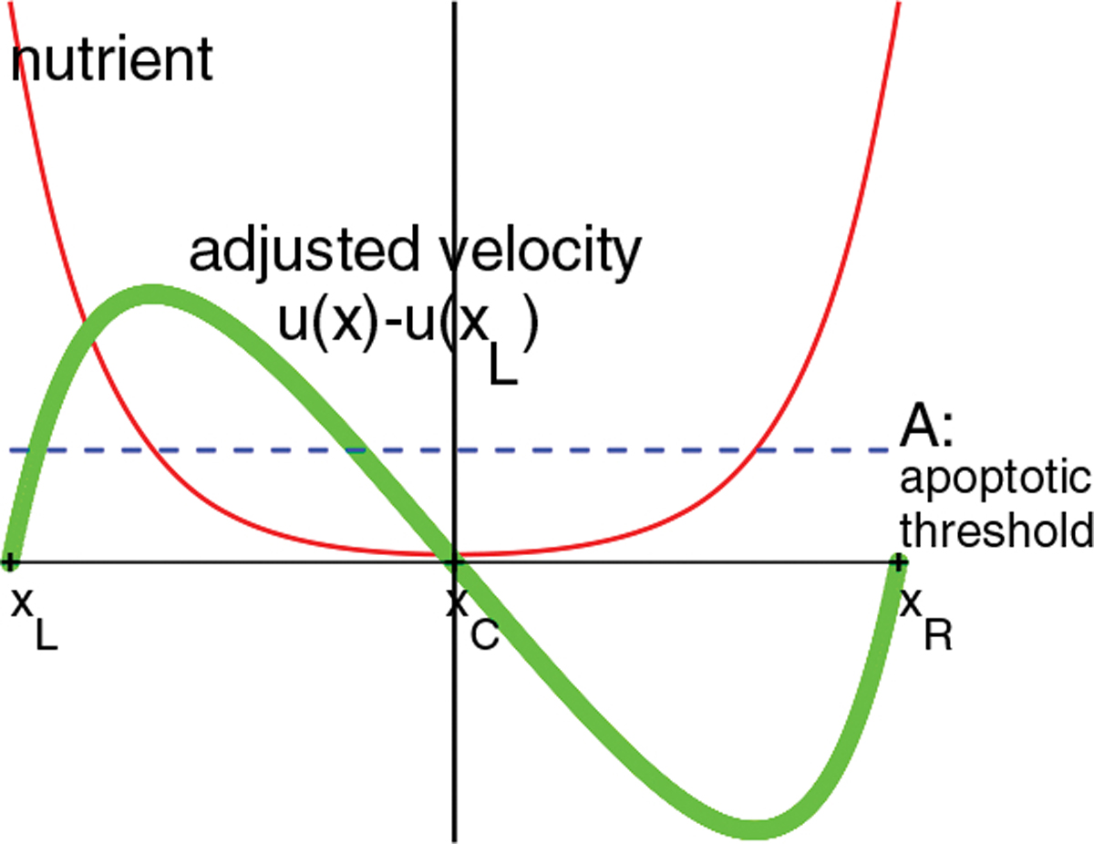
Solutions of nutrient and adjusted velocity u(x)−u(xL) when the tumor size is in the steady state. The tumor domain is the interval (x_L, x_R) where x_C is the center. The nutrient n(x) = cosh(x − x_C)/cosh(β) and is symmetric around the x = x_C vertical line. The adjusted $\text{velocity}=\frac{\text{sinh}\left(x-x_C\right)}{\text{cosh}(\beta )}-A\left(x-x_C\right)$ is symmetric around the tumor center point x_C

2.2. One dimensional simulation when K(x) = e^cx

First, we consider a special case where K(x) = exp(cx), where c is a constant. According to the calculations in (Sweidan et al. 2020), the velocity in the tumor for x ∈ (x_L, x_R) is

$$\begin{gathered} u(x)=G\left(\frac{A}{c}-\frac{c}{c^2-1}+\frac{c^2}{c^2-1}\text{tanh}(\beta )\frac{1+e^{-2c\beta }}{1-e^{-2c\beta }}\right. \\ \left.+\frac{\text{sinh}\left(x-x_L-\beta \right)}{\text{cosh}(\beta )}-A\left(x-x_L\right)-2A\beta \frac{e^{-2c\beta }}{1-e^{-2c\beta }}\right). \end{gathered}$$ (23)

Thus, the velocities at the tumor boundary x = x_L, x_R are:

$$u\left(x_L\right)=G\left(\frac{A}{c}-\frac{c}{c^2-1}+\frac{\text{tanh}(\beta )}{c^2-1}\cdot \frac{1+\left(2c^2-1\right)e^{-2c\beta }}{1-e^{-2c\beta }}-\frac{2A\beta e^{-2c\beta }}{1-e^{-2c\beta }}\right),$$ (24)

$$u\left(x_R\right)=G\left(\frac{A}{c}-\frac{c}{c^2-1}+\frac{\text{tanh}(\beta )}{c^2-1}\cdot \frac{2c^2-1+e^{-2c\beta }}{1-e^{-2c\beta }}-\frac{2A\beta }{1-e^{-2c\beta }}\right).$$ (25)

At the steady state of the tumor size, u(x_L) = u(x_R) and the entire tumor velocity is

$$u_{tbs}=G\frac{(A-1)c^2+c\text{tanh}(\beta )\coth (c\beta )-A}{c\left(c^2-1\right)}.$$ (26)

Because this velocity is a constant in both space and time, the entire tumor domain moves with a steady velocity. Since it is an odd function of c, when c switches sign, the tumor will change its direction but grows with the same speed.

Note that the velocity u(x) in (23) can be rewritten as $u(x)=\widehat{u}\left(x-x_L\right)$ where

$$\begin{gathered} \widehat{u}(z)=G\left(\frac{A}{c}-\frac{c}{c^2-1}+\frac{c^2}{c^2-1}\text{tanh}(\beta )\frac{1+e^{-2c\beta }}{1-e^{-2c\beta }}\right. \\ \left.+\frac{\text{sinh}(z-\beta )}{\text{cosh}(\beta )}-Az-2A\beta \frac{e^{-2c\beta }}{1-e^{-2c\beta }}\right). \end{gathered}$$ (27)

Therefore, the velocity profile over the tumor domain is invariant. In other words, the velocity field is identical when the tumor domain moves from one location to another. Integration of p′(x) = −u(x)/K(x) with K = e^cx, $u(x)=\widehat{u}\left(x-x_L\right)$, and p(x_L) = 0 yields

$$p(x)=-{\int }_{x_L}^x\frac{\widehat{u}\left(x-x_L\right)}{e^{cx}}dx=-e^{-c{x}_L}{\int }_0^s\frac{\widehat{u}(s)}{e^{cs}}ds,$$ (28)

where s = x − x_L. This indicates the pressure field over the tumor domain is also identical up to a multiplicative factor $e^{-c{x}_L}$ when the tumor domain moves in the steady state.

The steady state tumor boundary velocity in (26) is shown in Fig. 2 for several values of 0 < A < 1 and c > 0 in K(x) = e^cx. It is clear from these numerical values that the velocity is always negative in these cases, thus in the negative gradient direction of K.

Fig. 2.

Tumor velocity in (26) for some values of A and K = e^cx. G = 1

Next, we use the numerical scheme developed in (Zheng and Sweidan 2019; Sweidan et al. 2020) to solve the system in Sect. 2.1 and illustrate the numerical results for A = 0.2 and K(x) = e^0.5x. The initial position of the tumor is $\left(-\frac{3}{11},\frac{59.6}{11}\right)$. From the results presented in Fig. 3a, the pressure has a much larger gradient at the front (x = x_L) than at the rear (x = x_R). In the steady state of the tumor size, the tumor domain moves with a constant negative velocity (Fig. 3b).

Fig. 3.

One dimensional simulation. G = 1, A = 0.2, K = e^0.5x. a plots of nutrient, velocity, and pressure at t = 20. b is the boundary positions vs time.

2.3. One dimensional tumor growth when conductivity K(x) is piecewise constant

We present more examples in the one-dimensional case with G = 1, A = 0.2. In this case, the steady tumor size is 10. First, we set up a step function for the conductivity

$$K_1(x)=5+\text{tanh}\left(\frac{x+5}{ϵ}\right)+\text{tanh}\left(\frac{x}{ϵ}\right)+\text{tanh}\left(\frac{x-5}{ϵ}\right)+\text{tanh}\left(\frac{x-10}{ϵ}\right),$$ (29)

where ϵ = 0.05, whose graph is shown in Fig. 4a. The initial tumor domain is (7.5, 17.5), so the tumor size is already in the steady state. Under this step function, the tumor domain moves to the left without changes in its size (Fig. 4b). The final tumor domain is (−15, −5) and thus is completely located in a region with constant, lowest value of K₁.

Fig. 4.

Step function case. a step function in (29). b tumor boundary evolution. c nutrient, pressure, velocity profiles at t = 800

Second, we set up an L-step conductivity function

$$\begin{gathered} K_2(x)=6-\text{tanh}\left(\frac{x+10}{ϵ}\right)+\text{tanh}\left(\frac{x+5}{ϵ}\right)+\text{tanh}\left(\frac{x}{ϵ}\right)+\text{tanh}\left(\frac{x-5}{ϵ}\right) \\ +\text{tanh}\left(\frac{x-10}{ϵ}\right), \end{gathered}$$ (30)

where ϵ = 0.05, whose shape is shown in Fig. 5a. Note the lowest K₂-region is the interval (−10, −5). The tumor starts the same position as in the step function K₁ case but its final state is (−12.5, −2.5). That is, the tumor center, x = −7.5, coincides with the center of the lowest K₂-region. Note the conductivity in the tumor domain is an even function with respect to the tumor center. Therefore, the necessary condition (17) for the zero entire tumor velocity is achieved in the final state.

Fig. 5.

L-step function case. a L-step function in (30). b tumor boundary evolution. c nutrient, pressure, velocity profiles at t = 800

Next, to examine the preference of the tumor to grow to low conductivity region, we design the following K function

$$K_3(x)=-\left(1-\frac{h}{2}\right)\text{tanh}\left(\frac{x+2.5}{ϵ}\right)+\text{tanh}\left(\frac{x-2.5}{ϵ}\right)+3-\frac{h}{2},$$ (31)

where ϵ = 0.05 and h is the drop from the right bank to the left bank, as shown in Fig. 6a. The right bank is in the interval (2.5, 10) and its K-value is kept as 3. The bed occupies the region (−2.5, 2.5) and its K-value is 1. The left bank is (−10, −2.5) and its K-value is 3 − h. The initial tumor domain is set as (−5, 5). The simulations are implemented for several values of h ∈ [0, 2] and each simulation runs to time t = 500 to ensure that the tumor evolves to a steady state. The final tumor position with respect to the jump value h is summarized in Fig. 6b. It is observed that the tumor size remains as 10 in all the simulations. When h = 0, that is, the left and right banks having the same conductivity, the final tumor domain takes the central position and has the same length on both banks. When 0 < h < 2, the lengths of the tumor on both banks are nonzero. However, with the increase of the jump, the length on the left bank increases and that on the right bank decreases (see Fig. 6c). When h = 2, the left bank levels with the bed and the final tumor domain is (−7.5, 2.5), thus entirely growing out of the right bank. The necessary condition (17) for the zero entire tumor velocity is satisfied in all these states. Although this example is quite complicated, it still demonstrates the tendency of tumor growth towards the region of low conductivity.

Fig. 6.

a K function with jump defined in (31). The middle low value region (bed) is (−2.5, 2.5). The K value on the right bank is kept as 3. b final tumor domain vs jump value h. c lengths of the final state tumor on both banks vs jump h

2.4. Some extreme cases in one-dimensional tumor growth

To provide more insights to the impact of inhomogeneous conductivity on the tumor growth, we consider a few extreme cases: the apoptosis rate A = 0 and the nutrient n = 0. Note that when G = 0, the divergence of velocity is zero, which leads to −∇ · (K(x)∇ p(x)) = 0. Along with the Dirichlet boundary condition ${\left.p\right|}_{\partial \mathrm{\Omega }}=0$, the pressure has a unique zero solution, which results in the zero solution of the velocity. Thus, in the case of G = 0, the tumor domain does not move.

In the first extreme case, A = 0, the tumor cells never die. We set G = 1 and K(x) = e^cx. Following the calculation in (18), we get $\frac{d\beta }{dt}=\text{tanh}(\beta )$. The solution is sinh(β(t)) = sinh(β₀)e^t. Since sinh is a monotonically increasing function, it is easy to see that as t → ∞, the tumor size increases to infinity. When β ≫ 1, sinh(β) ≈ e^β/2 and (x_R − x_L)(t) ≈ 2t +2 ln(2 sinh(β₀)). So the tumor size expands to infinity linearly. To find out the speed of the left and right boundaries, we performed some numerical simuations with the initial tumor position (−3/11, 59.6/11). From the result in Fig. 7a for c = 0.5, the tumor expands in both directions. However, the right boundary moves faster to the right than the left boundary moving to the left. The change of the boundary speeds with respect to c is summarized in Table 1. As c tends to zero, the magnitudes of boundary velocity approach the same. When c > 0, the right boundary always moves faster than the left boundary. The larger value of c, the larger difference between the two boundary velocities.

Fig. 7.

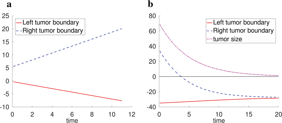
a boundary evolution when A = 0 and K(x) = e^0.5x. b boundary and tumor size evolution when nutrient n = 0 and K(x) = e^0.5x.

Table 1.

Left and right tumor boundary velocities when A = 0

c in K (x) = ecx	Left boundary velocity	Right boundary velocity
0.5	−0.67	1.33
0.25	−0.80	1.20
0.125	−0.89	1.11
0	−1	1

In the second extreme case, n(x, t) =R 0, that is, the nutrient is depleted. The equations u′ = −GA and $\frac{d\left(x_R-x_L\right)}{dt}={\int }_{x_L}^{x_R}{u}^{\prime }dx=-GA\left(x_R-x_L\right)$ lead to (x_R − x_L)(t) = (x_R − x_L)(0)e−^GAt. So the tumor size shrinks to zero exponentially. In the numerical simulations, we take the initial tumor position as (−35, 35) and the result is shown in Fig. 7b for the parameters G = 1, A = 0.2, and K(x) = e^0.5x. The average left and right boundary velocities for several values of c in K = e^cx functions are shown in Table 2. When c > 0, the right boundary always moves faster than the left boundary, and the gap between the boundary speed increases as c value becomes larger.

Table 2.

Left and right tumor boundary average velocities when nutrient n = 0, G = 1. Average velocity=total displacement/time duration

c in K (x) = ecx	Left boundary average velocity	Right boundary average velocity
0.5	0.32	−3.06
0.25	0.54	−2.84
0.125	0.83	−2.55
0	1.69	−1.69

In summary, the results in this subsection demonstrate when the whole tumor is expanding or shrinking in one dimensional space, the two tumor endpoints move in the opposite directions but the motion in the high conductivity region is faster than that in the low conductivity region.

3. Two dimensional simulations

In this case, we solve the equations (1), (4), (5), (6), (7) in two dimension. The evolution of the tumor boundary is implemented by the level-set method. Let ψ be the signed distance function to the tumor boundary ∂Ω(t), thus $\partial \mathrm{\Omega }(t)=\left\{\mathbf{x}\in {ℝ}^2:\psi (\mathbf{x})=0\right\}$. Then

$$\frac{\partial \psi }{\partial t}+\mathbf{u}\cdot \nabla \psi =0.$$ (32)

We used the interface-fitted adaptive mesh method developed in (Zheng and Lowengrub 2016) to solve this problem and evolve the tumor boundary. To confirm convergence, all the simulations were performed with three different mesh sizes and the convergence was observed in all the cases. The results presented here are from the finest resolution, where the smallest mesh size of the adaptive mesh is h = 0.01.

3.1. Perturbed circular tumor under radially symmetric conductivity

If both the initial tumor shape and the conductivity are radially symmetric, the tumor always grows in the radially symmetric manner irrelevant to the conductivity. Indeed, the solution uniqueness implies the nutrient, pressure, and velocity are all radially symmetric. Denote r as the polar radius. The radial component of the velocity u_r satisfies $\frac{1}{r}\frac{\partial \left(r{u}_r\right)}{\partial r}=G(n(r)-A)$. Along with the non-singular condition u_r(0) = 0, the velocity field is fully determined.

In the first group of nontrivial two-dimensional simulations, the initial tumor boundary is set as a perturbed circle: (2 + 0.1 cos(2s), 2 + 0.1 sin(2s)), s ∈ [0, 2π]. The other parameters are G = 20, A = 0.5, τ = 1. When K = 1, the linear analysis in (Cristini et al. 2003) shows the tumor growth is unstable, which agrees with the numerical solution (Fig. 8d) produced by the method used in this work (the direct comparison is given in (Zheng and Lowengrub 2016)). Here, we choose the conductivity as K = exp(cr), where c is a constant. The evolutions of equivalent tumor radii and shapes for some values of c are shown in Fig. 8. When c ≥ 0.6, the tumor grows to a disk of radius 3.324, which is the steady state radius when the initial tumor boundary is a circle. But when c ≤ 0.5, the tumor volume increases with time and some bulbs are formed that merge at a finite time, where the volume increase rate is higher and the merging time is earlier for smaller c values,

Fig. 8.

a evolution of equivalent tumor radius for the conductivity K = exp(cr). A curve stops when the tumor bulbs merge or one part of the tumor grows out of the computational domain [−6, 6]×[−6, 6]. b–e evolution of tumor shape with different conductivity K

According to the discussion in (Zheng et al. 2005), the formation of bulbs is produced by diffusion instability because the bulbs possess greater perimeter to area ratios, which allow them to be exposed to more nutrient within a unit tumor area diffusing from the boundary than a flat region. This mechanism drives the bulbs to grow larger and larger. On the other hand, according to the findings in the one dimensional case, the conductivity K = exp(cx) with c > 0 would induce the inward growth and the counterpart with c < 0 would induce outward growth. Both the diffusion instability and the directed growth induced by conductivity exist, sometimes competing and sometimes cooperating, in these simulations.

In particular, when the conductivity increases with radius and has a sufficiently large gradient magnitude (c ≥ 0.6), the tumor grows to a stable disk centered at the origin with the initial perturbation vanished. In this case, the inward growth suppresses the diffusion instablility. When the increasing conductivity has a sufficiently small gradient magnitude (0 < c ≤ 0.5), the diffusion instability exceeds the inward growth in the competition and thus the tumor grows to an unstable phase but with a slower volume increase rate compared with the K = 1 case, where the conductivity has no effect. Finally, when the conductivity decreases with radius (c < 0), the diffusional instability is enchanced by the conductivity induced outward growth and thus leads to ever faster unstable growth.

3.2. Circular tumor under non-radially symmetric conductivity

We fix G = 1, A = 0.8. In the case of a circular tumor, the steady state radius is approximately 1.47. We use this value as the initial radius of a tumor which is a circle centered at (0, 0). The conductivity is chosen as

$$K(x,y)=\exp (4x+2y).$$ (33)

Thus, its negative gradient direction is (−4, −2) at any point in space.

The simulation results of the zero surface tension are shown in Fig. 9. Figure 9a shows the path of tumor center with different line types indicating different directions. From the temporal snapshots of the tumor’s pressure field and boundary velocity depicted in Fig. 9b–d, we see that the tumor domain moves along the (−4, −2) direction from t = 0 to t = 14 and at the same time the tumor is bent forward because the speed on the center rear of path is larger than on the wings. However, after t = 14, the two bulbs at the back of the tumor grow larger in the backward direction, which pulls the tumor center back towards (0, 0). A little after time t = 31, the two bulbs are ready to merge.

Fig. 9.

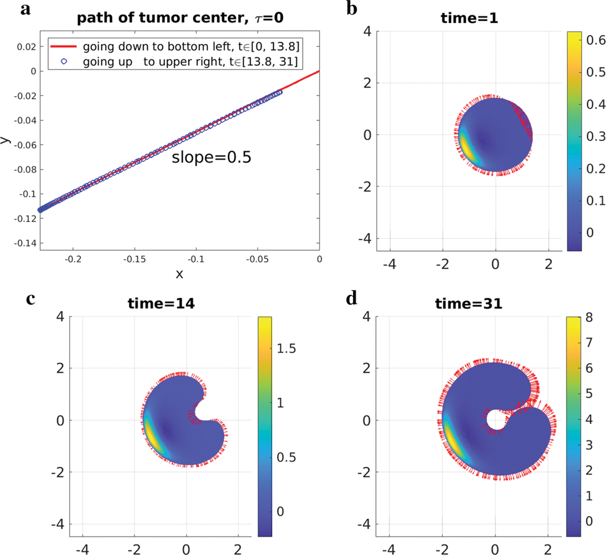
τ = 0 case. a path of tumor center. b, c, d pressure field and boundary velocity. The vectors are the velocity on the tumor boundary. The maximum magnitudes of velocity of these pictures are between 0.04 and 0.08

When the surface tension is τ = 0.05, 0.2, 0.5, 1, 4 or 8, the tumor center moves along the negative gradient direction of K without any reverse motion up to time t = 120 (Fig. 10a). The equivalent tumor radii decrease initially for all the positive surface tension values, more rapidly when the surface tension is larger (Fig. 10b). Afterwards the radii increase roughly linearly in time. Both the x and y coordinates of the tumor center evolve linearly in time (Fig. 10c, d).

Fig. 10.

a path of tumor center vs time where the arrow indicates the tumor center movement direction. All the cases when τ > 0 are roughly the same. b evolution of equivalent tumor radii. c, d evolution of tumor center

When τ = 0.05,0.5,8, the tumor morphology, pressure field, and velocity field on the tumor boundary at some later times of tumor growth are shown in Fig. 11. Some morphology snapshots can be found in Fig. 12. With the increase of surface tension, the tumor tends to keep a more compact form with less bulbs.

Fig. 11.

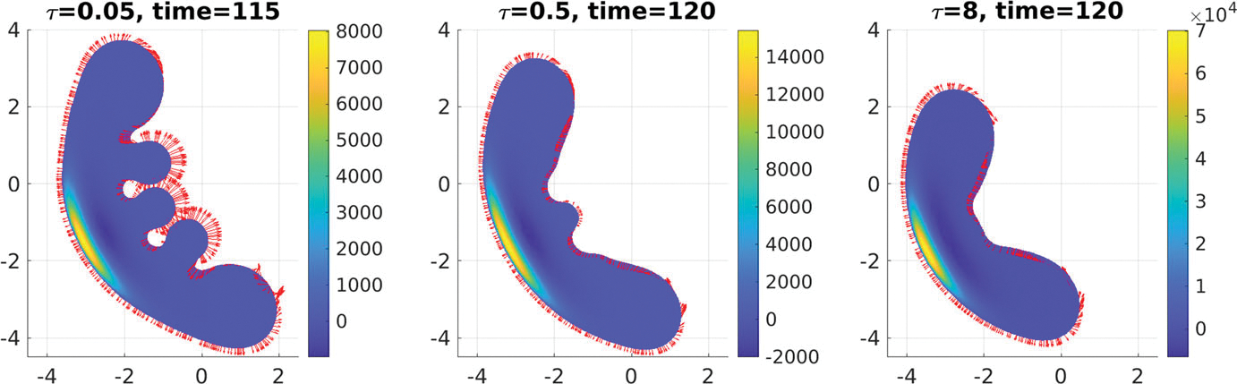
Comparison of tumor pressure and velocity fields under different surface tensions

Fig. 12.

Snapshots of tumor evolution in the same axes. When τ = 0, t = 0, 6, · · ·, 30, 31. When τ = 0.05, t = 0, 10, …, 110, 115. When τ = 0.5 and 8, t = 0, 10, · · ·, 120.

There are some similarities about the results between the one-dimensional (1-D) and two-dimensional (2-D) simulations in Sect. 3.2². The first is that the tumor grows towards the negative gradient direction of conductivity. The second is that the tumor thickness in 2-D case or the tumor size in 1-D case is almost steady in time. In 2-D case, when the surface tension is positive, the tumor roughly adopts a crescent shape at the later stage and one portion of the boundary forms a clear advancing front. The tumor thickness is not only quite uniform across the front but also roughly constant in time (by visual examination). In 1-D case, the tumor size is fixed once the tumor reaches the steady size. The third similarity is the pressure distribution after the center of the front, as shown in Fig. 13. It jumps sharply from a nearly zero value on the tumor boundary to a large positive value after the front, then drops to a large negative value in the middle, and then slowly goes up to zero to the rear boundary. It resembles the pressure field in the 1-D case in Fig. 3a.

Fig. 13.

Pressure field after the advancing front at time t = 120 when surface tension τ = 8. a top view. b side view perpendicular to the growth direction. The tumor domain moves to the left

4. Discussion

In this work, we discovered a phenomenon from one and two dimensional numerical simulations using a Darcy’s law model of tumor growth that the tumor tends to grow to regions of low hydraulic conductivity, when the tumor morphology is steady. The examples in two-dimensional space indicate the tumor would grow in the negative gradient direction of the conductivity. This phenomenon is accompanied with a critical condition: in one-dimensional case the tumor size is fixed, and in two-dimensional case the tumor thickness in the direction of the growth is roughly fixed. Especially in one-dimensional case, we proved in Theorem 1 part (iv) that when the tumor size is steady, the tumor must favor growth towards lower conductivity regions if the conductivity is strictly increasing or decreasing in space. If the tumor size is not fixed, then this phenomenon might not be true. For example, when the cell death is turned off, the tumor size grows to infinity and the two boundaries expand outwards but the boundary in the larger conductivity region moves faster.

The similarities of the one- and two-dimensional cases make it plausible to look into the one-dimensional case to understand this phenomenon. Two mechanisms stand out as follows.

1. The special inward flow pattern inside the tumor when the size is steady. The velocity field relative to the tumor center³ is towards the tumor center and symmetric around the center. It is completely determined by the nutrient distribution and cell division and death. This leaves only one degree of freedom for Darcy’s law to play around: the entire tumor domain moves to left or right, or stays still.

2. The faster flow speed in higher conductivity regions due to Darcy’s law. Remark 3 states when the tumor size is steady, the speed is faster on a point of higher conductivity than on its symmetric point across the center (not including boundary points). The extreme cases in Sect.2.4 demonstrate when the tumor size is not steady, the boundary in the higher conduction region travels faster. This is a nature of Darcy’s law because of |u| = K|∇ p|, that is, under the same pressure gradient magnitude, the larger conductivity yields the larger flow speed.

To understand how these mechanisms generate this phenomenon, we design a comparison experiment. A tumor domain is chosen as (−5, 5). Let G = 1, A = 0.2. The tumor size is steady with these parameters. At first, we set the conductivity K = 1 everywhere. As shown in Fig. 14a, the pressure profile is symmetric around the tumor center. However, when the conductivity on the right half is suddenly changed to 11 while the conductivity on the left is kept the same as before, Fig. 14b shows the velocity on the right increases the negative magnitude. At the same time, the pressure from the right of the center is larger than from the left. This implies the flow from the right exerts compressing force to the left. The pressure reaches the maximum value near the left endpoint because the conductivity is lowest there and an extra force is required to push the left endpoint to move in the same speed as the right endpoint. Therefore, we conclude the growth to lower conduction regions, under steady morphology, is induced by the pushing force from the faster inward flow in the higher conductivity regions.

Fig. 14.

Comparison of velocity and pressure fields with uniform conductivity (a) and with higher conductivity on the right half of tumor domain (b)

The finding that the tumor grows towards regions of low conductivity is deduced from both mathematical analysis and numerical experiments of the growing dynamics. Although there are many experiments evaluating single cell movement through a heterogeneous ECM (e.g. (Harley et al. 2008; Wolf et al. 2013)), we have not seen any biological or clinical reports on the collective movement of proliferating cells in response to inhomogeneous conductivity. However, we believe this work is meaningful for the cancer research community. Above all, the ECM has a high degree of heterogeneity due to the intrinsic disorder of the fiber network (Malandrino et al. 2018). Therefore, if this finding can be verified experimentally, then it can be used as a basis for further development of mathematical models and design of potential therapy. One possible experimental setup to test this finding is using a nondegradable and nondeformable substrate as in (Wolf et al. 2013). On the other hand, if this prediction is not observed in experiments given the same assumptions of this model, it would be an opportunity to consider the range of validity of this model.

The existing understanding of collective cancer invasion (e.g., (Wu et al. 2021)) involves many features such as distinct cell phyenotypes at leading and trailing edges, and pericellular proteolysis mediated ECM reorganization, neither of which is present in this work. In contrast, this work shows that the motion under Darcy’s law could solely drive the tumor to spread from high to low ECM conductivity regions. Thus, the mechanism, if verified in cancer biology, would unveil a new mode of collective tumor invasion that may lead to complications of cancer therapy. For instance, in all the possible responses to a therapy, there is a special category named stable disease (Therasse et al. 2000), where the tumor could stay in relatively the steady size (between 30% decrease and 20% increase since the initial baseline measurement) over 6 to 8 weeks. Under this mechanism, the tumor may spread to nearby tissue or organs, which would increase the risk of metastasis and the difficulty of prognosis.

Note that the tumor boundary remains smooth for all the two-dimensional simulations until the possible merging occurs, which is also true when the conductivity is a constant in space (see (Cristini et al. 2003)). This tumor model has a strong correlation with the Hele-Shaw flow problem, where Darcy’s law is applied to the motion of incompressible viscous fluid between two parallel horizontal plates separated by a thin gap. The fluid domain is expanding or shrinking due to a point source or sink in the center of the domain. The cusp singularity (a zero angle corner) occurs in Hele-Shaw flows for shrinking fluid with zero surface tension (Howison 1986). This type of singularity is not observed in this work even when the tumor surface tension is zero. We postulate this is because in this tumor growth model, the nutrient level is always set as one on the tumor boundary and thus whenever A < 1, the volume change rate ∇ · u = G(n − A) is always positive near the tumor boundary. Therefore, this tumor model seems more similar to the expanding Hele-Shaw problem near the tumor boundary. According to (Howison 1986), the expanding Hele-Shaw problem is well-posed and the boundary is analytic as long as the domain keeps simply connected, which agrees well the simulations in this work. But certainly it will be worthwhile to perform rigorous theoretical and numerical analysis in this direction.

Appendix

Basics of Darcy’s law and mass transport in porous media

This section extracts some information useful for our discussion from a classic book by Bear (Bear 1972). Above all, notice that in the continuum approach of fluid dynamics in porous media, all the kinematic and dynamic variables are defined as averaged values in a proper volume (representative elementary volume), such as porosity, velocity, pressure. Darcy’s law for homogeneous fluid flowing through inhomogeneous isotropic porous media can be written as

$$\mathbf{q}=-K\nabla \phi ,$$ (34)

where q is the specific flux with dimension length/time, measuring the volume of fluid discharged through porous media per unit area per unit time. Let ϕ be the porosity (the fraction of pores or void space in a unit volume) and u be the flow velocity of the fluid in the pores, then relation between specific flux and velocity is expressed with the following Dupuit-Forchheimer equation,

$$\mathbf{q}=\varphi \mathbf{u}.$$ (35)

The value of ϕ is between 0 and 1 and often expressed by a percentage. The porosity is defined in such a way that around any point in the porous media, the void space fraction is ϕ. The coefficient K = K(x), $\mathbf{x}\in {ℝ}^3$, is the hydraulic conductivity and a scalar variable for inhomogeneous isotropic media. Its expression is

$$K=\frac{\rho gk}{\mu },$$ (36)

where ρ is the fluid density, g is the gravity acceleration, k is the intrinsic permeability (dependent solely on the property of the solid matrix) with dimension length², μ is the dynamic viscosity of the fluid. Thus, the dimension of K is length/time. The quantity φ is the piezometric or hydraulic head and given by

$$\phi =\frac{p}{\rho g}+z.$$ (37)

Here, p is hydrostatic pressure and z is the height. All these quantities with their dimensions are listed in Table 3. Using relation (35), the Darcy’s law (34) can be rewritten as

$$\mathbf{u}=-\frac{K}{\varphi }\nabla \phi .$$ (38)

Table 3.

Quantities used in Darcy’s law for porous media. Here the units are the ones usually used in groundwater hydrology

Symbol	Meaning	Dimension	Unit
q	specific flux in the whole porous media, q = ϕu	length/time	cm/s
K	hydraulic conductivity, K = ρgk/μ	length/time	cm/s
k	intrinsic permeability	length2	2 cm
φ	piezometric head, φ = p/(ρg) + z	length	cm
u	flow velocity in empty space	length/time	cm/s
ϕ	porosity or fraction of empty space	dimensionless
μ	fluid dynamic viscosity	force·time/length2	dyn·s/cm2.
ρ	fluid density	mass/volume	g/cm3
g	gravitational acceleration	length/time2	cm/s2
p	hydraulic pressure	force/area	dyn/cm2
z	height	length	cm

The mass balance equation for the tumor cell component according to (Bear 1972) (equation 4.3.1 therein) is

$$\frac{\partial (\rho \varphi )}{\partial t}+\nabla \cdot (\rho \varphi \mathbf{u})=I_t,$$ (39)

where I_t is the tumor cell source term. Under the assumption of constant density ρ and fixed porosity in time, $\frac{\partial (\rho \varphi )}{\partial t}=0$. The source of tumor cells given in (Cristini et al. 2003) is ρG(n − A), where G is the division rate and A is the apoptotic threshold. Because the tumor cell source term must be only present in the void space, therefore, I_t = ϕρG(n − A). Then the mass balance equation is reduced to

$$\nabla \cdot (\varphi \mathbf{u})=\varphi G(n-A).$$ (40)

In (Cristini et al. 2003), the mass equation is simply

$$\nabla \cdot \mathbf{u}=G(n-A).$$ (41)

Compared with (40), this must be done by assuming ϕ is a constant in space. For the sake of simplicity and comparison, we accept the assumption here.

Define $\tilde{p}=\frac{\phi }{\varphi }$ and use the definition of K in (36), then (38) becomes

$$\mathbf{u}=-K\nabla \tilde{p}.$$ (42)

Ignoring z in (37) and dropping the tilde for $\tilde{p}$, we get (1).

References

- Bazaliy BV, Friedman A (2003) A free boundary problem for an elliptic–parabolic system: application to a model of tumor growth. Commun Partial Differ Equa 28:517–560. 10.1081/PDE-120020486 [DOI] [Google Scholar]
- Bear J (1972) Dynamics of fluids in porous media. Dover [Google Scholar]
- Brace WF (1977) Permeability from resistivity and pore shape. J Geophys Res 82:3343–3349. 10.1029/JB082i023p03343 [DOI] [Google Scholar]
- Byrne HM, Chaplain MAJ (1996) Modelling the role of cell-cell adhesion in the growth and development of carcinomas. Math Comput Model 24:1–17. 10.1016/S0895-7177(96)00174-4 [DOI] [Google Scholar]
- Byrne HM, Chaplain MAJ (1997) Free boundary value problems associated with the growth and development of multicellular spheroids. Eur J Appl Math 8(6):639–658. 10.1017/S0956792597003264 [DOI] [Google Scholar]
- Caliari SR, Harley BAC (2011). 2.216.4.3. Cell Motility, in the book Comprehensive Biomaterials, Editor-in-Chief: Paul Ducheyne, Elsevier [Google Scholar]
- Cristini V, Lowengrub JS, Nie Q (2003) Nonlinear simulation of tumor growth. J Math Biol 46(3):191–224. 10.1007/s00285-002-0174-6 [DOI] [PubMed] [Google Scholar]
- Cristini V, Frieboes HB, Gatenby R et al. (2005) Morphologic instability and cancer invasion. Clin Cancer Res 11(19):6772–6779. 10.1158/1078-0432.CCR-05-0852 [DOI] [PubMed] [Google Scholar]
- Frieboes HB, Zheng X, Sun CH, Tromberg B, Gatenby R, Cristini V (2006) An integrated computational/experimental model of tumor invasion. Cancer Res 66(3):1597–1604. 10.1158/0008-5472.CAN-05-3166 [DOI] [PubMed] [Google Scholar]
- Friedman A, Reitich F (2001) Symmetry-breaking bifurcation of analytic solutions to free boundary problems: an application to a model of tumor growth. Trans Am Math Soc 353(4):1587–1634. 10.1090/S0002-9947-00-02715-X [DOI] [Google Scholar]
- Friedman A (2008) A multiscale tumor model. Interfaces Free Bound 10:245–262. 10.4171/IFB/188 [DOI] [Google Scholar]
- Friedman A, Hu B (2006) Asymptotic stability for a free boundary problem arising in a tumor model. J Differ Equa 227(2):598–639. 10.1016/j.jde.2005.09.008 [DOI] [Google Scholar]
- Gibson LJ, Ashby MF (1997) Cellular solids: structure and properties. In: Clarke DR, Suresh S, Ward IM (eds) Cambridge solid state science series. Cambridge University Press, Cambridge [Google Scholar]
- Giussani M, Triulzi T, Sozzi G, Tagliabue E (2019) Tumor extracellular matrix remodeling: new perspectives as a circulating tool in the diagnosis and prognosis of solid tumors. Cells 8(2):81. 10.3390/cells8020081 [DOI] [PMC free article] [PubMed] [Google Scholar]
- Giverso C, Ciarletta P (2016) On the morphological stability of multicellular tumour spheroids growing in porous media. Eur Phys J E 39(10):1–11. 10.1140/epje/i2016-16092-7 [DOI] [PubMed] [Google Scholar]
- Greenspan H (1976) On the growth and stability of cell cultures and solid tumors. J Theor Biol 56(1):229–242. 10.1016/s0022-5193(76)80054-9 [DOI] [PubMed] [Google Scholar]
- Harley BAC, Kim H-D, Zaman MH et al. (2008) Microarchitecture of three-dimensional scaffolds influences cell migration behavior via junction interactions. Biophys J 95(8):4013–4024. 10.1529/biophysj.107.122598 [DOI] [PMC free article] [PubMed] [Google Scholar]
- Howison SD (1986) Cusp development in Hele–Shaw flow with a free surface. SIAM J Appl Math 46(1):20–26. 10.1137/0146003 [DOI] [Google Scholar]
- Lowengrub JS, Frieboes HB, Jin F et al. (2010) Nonlinear modeling of cancer: bridging the gap between cells and tumors. Nonlinearity 23:R1–R91. 10.1088/0951-7715/23/1/r01 [DOI] [PMC free article] [PubMed] [Google Scholar]
- Malandrino A, Mak M, Kamm RD, Moeendarbary E (2018) Complex mechanics of the heterogeneous extracellular matrix in cancer. Extreme Mech Lett 21:25–34. 10.1016/j.eml.2018.02.003 [DOI] [PMC free article] [PubMed] [Google Scholar]
- Moura Neto F, Melo S (2001) Darcy’s law for a heterogeneous porous medium. J Porous Media. 10.1615/JPorMedia.v4.i2.60 [DOI] [Google Scholar]
- O’Brien FJ, Harley BA, Yannas IV, Gibson LJ (2005) The effect of pore size on cell adhesion in collagen-gag scaffolds. Biomaterials 26(4):433–441. 10.1016/j.biomaterials.2004.02.052 [DOI] [PubMed] [Google Scholar]
- O’Brien FJ, Harley BA, Waller MA et al. (2007) The effect of pore size on permeability and cell attachment in collagen scaffolds for tissue engineering. Technology and Health Care 15(1):3–17. 10.3233/THC-2007-15102 [DOI] [PubMed] [Google Scholar]
- Risler T (2013) Cytoskeleton and cell motility. In: Meyers R (ed) Encyclopedia of complexity and systems science. Springer, New York [Google Scholar]
- Sciumè G, Gray WG, Ferrari M et al. (2013) On computational modeling in tumor growth. Arch Comput Methods Eng 20:327–352. 10.1007/s11831-013-9090-8 [DOI] [Google Scholar]
- Shimolina LE, Izquierdo MA, López-Duarte I et al. (2017) Imaging tumor microscopic viscosity in vivo using molecular rotors. Sci Rep 7:41097. 10.1038/srep41097 [DOI] [PMC free article] [PubMed] [Google Scholar]
- Sweidan M, Chen X, Zheng X (2020) The Shortley–Weller scheme for variable coefficient two-point boundary value problems and its application to tumor growth problem with heterogeneous microenvironment. J Comput Appl Math 376:112874. 10.1016/j.cam.2020.112874 [DOI] [Google Scholar]
- Therasse P, Arbuck SG, Eisenhauer EQ et al. (2000) New guidelines to evaluate the response to treatment in solid tumors. JNCI J Natl Cancer Instit 92(3):205–216. 10.1093/jnci/92.3.205 [DOI] [PubMed] [Google Scholar]
- Wise SM, Lowengrub JS, Frieboes HB, Cristini V (2008) Three-dimensional multispecies nonlinear tumor growth-I: model and numerical method. J Theor Biol 253(3):524–543. 10.1016/j.jtbi.2008.03.027 [DOI] [PMC free article] [PubMed] [Google Scholar]
- Wolf K, Te Lindert M, Krause M et al. (2013) Physical limits of cell migration: control by ECM space and nuclear deformation and tuning by proteolysis and traction force. J Cell Biol 201(7):1069–84. 10.1083/jcb.201210152 [DOI] [PMC free article] [PubMed] [Google Scholar]
- Wu J, Jiang J, Chen B, Wang K, Tang Y, Liang X (2021) Plasticity of cancer cell invasion: patterns and mechanisms. Transl Oncol. 10.1016/j.tranon.2020.100899 [DOI] [PMC free article] [PubMed] [Google Scholar]
- Zheng X, Lowengrub J (2016) An interface-fitted adaptive mesh method for elliptic problems and its application in free interface problems with surface tension. Adv Comput Math 42(5):1225–1257. 10.1007/s10444-016-9460-5 [DOI] [Google Scholar]
- Zheng X, Sweidan M (2018) A mathematical model of angiogenesis and tumor growth: analysis and application in anti-angiogenesis therapy. J Math Biol 77(5):1589–1622. 10.1007/s00285-018-1264-4 [DOI] [PubMed] [Google Scholar]
- Zheng X, Sweidan M (2019) Analysis of ghost-fluid method with cubic extrapolation for two-point boundary value problem. Int J Numer Methods Appl 18(1):19–58. 10.17654/nm018010019 [DOI] [Google Scholar]
- Zheng X, Wise S, Cristini V (2005) Nonlinear simulation of tumor necrosis, neo-vascularization and tisse invasion via an adaptive finite-element/level-set method. Bull Math Biol 67:211–259. 10.1016/j.bulm.2004.08.001 [DOI] [PubMed] [Google Scholar]