Typical States and Their Risks for Mortgage Loans

Abstract

In this study, we construct a compartmental model that tracks the different states and their respective hazards for typical mortgage loans. We consider that an active mortgage loan could become delinquent in light of either common systemic risks or idiosyncratic risks in the job market. These two groups of employment-related perils jeopardize the sources of income underlying the mortgage monthly payments to lenders and could hurt the ability of mortgage loan borrowers to retire their debt. We also contemplate ongoing risks of a collapse in the housing market, which might transform the mortgage loan to be “underwater” and consequently diminish borrowers’ incentives to service the outstanding balance. We develop the necessary derivations, illustrate the functionality of the model over several hypothetical simulations and sensitivity analyses, suggest variable estimation specific guidelines, conclude, and discuss potential extensions for the proposed model.

Introduction

In this study, we construct a compartmental reliability model that tracks the conventional states of nature that lenders (of typical mortgage loans) encounter along with their respective common hazards. We shall consider that an active (or prompt) 30-year Fixed Rate Mortgage (FRM) loan could become delinquent during its lifetime because of three types of hazards. The first two classes of threats include systemic risks and idiosyncratic risks within the job market. These two groups of employment-related perils jeopardize the sources of income underlying the mortgage monthly payments to lenders and could hurt the ability of mortgage loan borrowers to retire their outstanding debt. We also contemplate ongoing risks of a collapse in the housing market, which might transform the mortgage loan to be “underwater” and consequently diminish borrowers’ incentives to service the outstanding mortgage balance.

We first develop the necessary derivations, based on eight possible states of nature and the routine transition rates (per unit of time) among them. We then illustrate the functionality of the proposed model over several hypothetical simulations and sensitivity analyses. These simulations aim to represent realistic scenarios, though they intentionally utilize somewhat exaggerated values, to stretch and inspect the limitations of the present model. Next, we uncover the overall behavior of this dynamic system. We also determine the expected lifetime of this mortgage loan (as the most likely time that the 30-year FRM loan will become delinquent), and further detect the critical points in time where the lender faces the highest risks. We also suggest variable estimation specific guidelines, conclude, and discuss potential extensions for the proposed model. We thus direct the current model to serve as an adaptable framework hence open for modifications with respect to diverse economic circumstances.

Lenders of conventional mortgage loans (not insured by the federal government and only secured by the collateral of a specified real estate property) are normally subject to three types of risks: interest rate risk, prepayment risk (also including the risk of refinance), and default risk. Interest rate risk arises when the rate on an Adjustable Rate Mortgage (ARM) decreases, leading to reduced monthly payments for a floating interest rate loan. Prepayment risk applies when the borrowers have both the ability and willingness to prematurely remove larger portions than scheduled of the (or even the entire) principal loan amount. In this event, lenders would also suffer from lower future interest payments (similar consequences occur when borrowers refinance the mortgage loan with dropping interest rates). However, these two situations do not result in delinquent mortgage loans (and subsequent foreclosures), as in the case of default risk, which in most instances impacts both principal and interest payments. Therefore, default risk is the major risk that habitually causes the larger monetary losses and the utmost legal complications to lenders. Thus, we shall focus hereafter on the root causes of default risk for FRM loans, and in particular for 30-year FRM loans. Traditionally, this class of mortgage loans is the most popular among first time homebuyers in the U.S., as well as in many other nations. Its attractiveness relies on the facts that it is amortized over a rather convenient horizon of 30 years, with 360 identical principal and interest monthly payments, and it provides stability and, relative to other types of loans, ease of budget planning to borrowers.

Nonetheless, the notion of default risk is rooted in several factual vulnerabilities. The first and obvious peril evolves from the potential risk that if mortgage loan borrowers lost their sources of income, they simply would not be able to pay back the remaining debt. This situation could arise because of either systemic risks or idiosyncratic risks in the job market. In addition, lenders face the risk that the housing market will collapse and consequently the value of the property underlying the mortgage loan will drop in value to below the outstanding balance on the mortgage. These (somewhat rare yet feasible) unfortunate circumstances may induce the borrower to default due to moral hazard. Furthermore, in this latter event, the lender must not only incur the costs of foreclosing but also must sell the underlying property at a price that fails to recoup the lender's investment.

We are therefore motivated to explore the various operational states (active and delinquent) along with their respective hazards (systemic risks and idiosyncratic risks in the job market and the risk of a collapse in the housing market) for 30-year FRM loans. This investigation could benefit mortgage lenders and associated financial institutions by enhancing the awareness of the deep roots of the regular risks and the underlying processes that could lead to mortgage delinquency and subsequent foreclosures. We contribute to the literature of risk management by presenting here a simple framework that examines the distinct types of failures in the realm of mortgage loans. The proposed model does not aspire to capture all of the feasible economic scenarios. Nonetheless, intrigued researchers can modify the present scheme to accommodate other related settings of mortgage lending.

The remainder of the study is organized as follows. In the next section, we provide a brief survey of the literature on mortgage delinquencies. In the third section, we assemble a quantifiable model that tracks the operational states and their respective risks for common mortgage loans. In the fourth section, we deploy several simulations and sensitivity analyses that provide further insight into our proposed model. In the fifth section, we provide some detailed estimation guidelines to the essential input variables. In the sixth section, we summarize, conclude, and suggest a few possible extensions and alternations of the current model.

Related Literature on Mortgage Delinquencies

To allow readers a broader view on the subject, to place the current study in the right context, and to highlight the contribution of the proposed model, we survey hereafter articles related to mortgage delinquencies. Because of its importance, this topic has attracted scholars’ attention over the past several decades. Early studies including von Furstenberg and Green (1974a, b), Morton (1975), Webb (1982), Campbell and Dietrich (1983), and Vandell and Thibodeau (1985) are the pioneers that examine how and which loans’ features and borrowers’ characteristics are associated with mortgage delinquencies. These articles find that household income and interest rates are more influential determinants than home equity in rationalizing delinquency, while home equity and borrowers’ ability to pay are more pronounced at a final foreclosure than among mortgage late payments. Households headed by minorities and income variability factors also contribute to mortgage delinquency rates, where loan-to-value ratio and the presence of junior financing further convey a positive impact on mortgage delinquency rates.

Quercia and Stegman (1992) provide a survey of past literature on residential mortgage defaults. Chinloy (1995) finds that loan-to-value ratio and income are the key determinants of mortgage delinquencies in the U.K. from 1983 to 1992. Ambrose and Capone (1996) empirically show that the length of the first “serious delinquency” (defined as 90 or more days) reduces the likelihood for a second serious delinquency. Calem and Wachter (1999) and Ambrose and Capone (2000) report that credit scores, the incentive structures of the lenders, and contemporary economic conditions can also affect mortgage delinquencies.

Ambrose and Capone (1998), Alexander et al. (2002), Pennington-Cross (2002, 2003), Calem et al. (2004), Cowan and Cowan (2004), Courchane et al. (2004), Capozza and Thomson (2005, 2006), Cutts and van Order (2005), Danis and Pennington-Cross (2005), Pennington-Cross and Chomsisengphet (2007), and Foote et al. (2008a, b) concentrate on delinquencies across Federal Home Administration (FHA) and subprime mortgage loans. These articles find that subprime borrowers are more likely to miss mortgage payments, when compared to prime mortgagers, because of unexpected life-cycle events such as death, illness, divorce, job loss, or sudden increase in mortgage interest rates on ARMs. These articles also document that subprime loans tend to default earlier and reach foreclosures in larger numbers, and they usually carry higher monetary losses compared to prime loans. Doms et al. (2007a, 2007b) describe how pockets of regional economic weakness pushed subprime borrowers into delinquency, while the speed of adjustments in house prices affected the incentives and opportunities for mortgage borrowers to avoid delinquencies and foreclosures. Foote et al. (2008a, b) further demonstrate how negative equity can lead to higher probability of home foreclosure.

Another fast-developing branch of the literature has emerged in the years following the financial crisis in the early 2000s. This outlet examines the harsh economic implications of the mounting mortgage delinquency rates. Among others, Mayer et al. (2009) discuss some facts and myths concerning the growth in mortgage defaults. Mian and Sufi (2009) identify the effects of the sharp increase in the supply of mortgage credit on the housing bubble as recorded from 2001 to 2005. Keys et al. (2010) explain how securitization weakened the motivation of lenders to screen loan applicants. Demyanyk and Hemert (2011) present the deterioration in loan quality from 2001 to 2006, while according to this study securitizers were, at least to some degree, aware of this gradual erosion in loan quality.

Kaufmann et al. (2011) also discover a long-term relationship between the percentage of U.S. mortgages that are 30 to 89 days past due and the interest rate on one-year ARMs, household expenditures on energy, nominal home prices, and rates of home ownership. Jiang et al. (2013a, b, 2014) study some problematic incentives stirring mortgage delinquency. The authors first present a contrast between ex-ante and ex-post relations between lenders and borrowers. In their later paper, the authors analyze mortgage delinquencies from 2004 to 2008 and highlight the two key problems underlying the recent mortgage crisis; a reliance on mortgage brokers who tend to originate lower-quality loans and a prevalence of low documentation loans, which incorporates a large scale of income falsification.

Beem (2014) highlights the determinants of mortgage defaults in the U.S. from 1999 to 2011 by stating that specific region and year also affect mortgage delinquency rates. Keys et al. (2014) use proprietary loan-level panel data, focus on agency loans with 60 or more days delinquent as their measure of delinquency status, and detect that a sizable decline in mortgage payments ($150 per month on average) causes a meaningful drop in mortgage defaults.1 Aron and Muellbauer (2006) introduce a theory-justified estimate of the proportion of mortgages in negative equity as a key driver of aggregate repossessions and arrears in the UK. Lin et al. (2016) further explain that due to their different social and economic background, immigrant households may not integrate well into the host society and therefore are more likely to be delinquent on mortgages than otherwise identical native-born households. Parnes (2018) detects signs of U.S. abnormal mortgage delinquencies from 2004 until 2010 that could have alerted lending institutions with housing crisis early symptoms.

Mortgage delinquencies evidently affect individual households, investors, securitizers, lending banks, different layers of the society, specific geographic regions, and even wide economies. Therefore, the ability to track the operational states and their respective risks for mortgage loans should earn the attention from lending institutions, bank audit companies, policy makers, supervisors, regulators, and professional real estate investors. As described in this brief literature review, there are numerous social and economic determinants for mortgage delinquencies and defaults. Nonetheless, these diverse factors can be customarily clustered into three fundamental groups of systemic risks, idiosyncratic risks, and housing market risks. We therefore focus hereafter on these three groups and assemble a generic risk model that tracks the universal risks for typical mortgage loans. We know of no other circulated study that presents a quantitative model along these lines or takes a parallel modeling approach.2

The Proposed Model

To portray a realistic setting for a customary mortgage loan, its different states, and their respective risks, we consider hereafter that a married couple takes a 30-year FRM from a lender. At the time of initiation of this highly popular mortgage loan among first-time home buyers, i.e., at time $\tau =0$, both spouses work and earn steady income, and the housing market is rather normal, in the sense that it has not experienced major obstructions or any significant depreciations to house prices recently. This very common form of mortgage loan for home purchasing can be continuously serviced as long as at least one person from the married couple still works, i.e., a single paycheck provided by any one of the spouses is sufficient to cover the monthly mortgage payments, and as long as the housing market does not sharply decline, hence house values do not rapidly fall.3

Over a long-term horizon such as thirty years, any one of the spouses can potentially lose his or her job and therefore his or her exclusive source of income because of either systemic risks or idiosyncratic risks. The systemic risks largely include massive layoffs due to reduction in force or structural downsizing of the respective employers and other business-related entities, a lasting contractionary economic cycle or a severe recession, which increases both the national and the local unemployment rates and simultaneously limits occupation opportunities, an outbreak of a pandemic such as the recent coronavirus, which could obliterate entire industries and subsectors for extended periods, and so forth.

Idiosyncratic risks in the job market often include developing chronic health conditions that prevent one from conducting his or her routine work duties, getting fired, having other personal issues and subsequently resigning from a job or abandoning other business initiatives, etc. We deem these systemic and idiosyncratic risks as fundamental and consequently irreparable or at least not redeemable in the foreseeable horizon.4 Apart from ordinary hazards in the job market, in case of a housing market crash, the mortgage loan may become “underwater,” hence the remaining principal of the mortgage loan is higher than the free-market value of the underlying home. Thus, regardless of the collective income earned by the couple and their ability to continue servicing the loan, in this case, the spouses have no equity left for credit and no real incentives to service the mortgage loan any longer, so they simply abandon their mortgage loan and walk away from their house. These ominous developments became widespread in the U.S. during the 2007–2008 financial crisis.

To assemble a tractable model for this common scenario we shall therefore assume that (1) at origination of this 30-year FRM loan both of the spouses work and the housing market is normal (i.e., house-values moderately appreciate or depreciate but they do not collapse), (2) the FRM loan becomes delinquent only when both spouses lose their jobs and/or if the housing market has recently crashed, (3) loss of employment (and thus income) is irreversible and may occur in light of either systemic risks or idiosyncratic risks in the job market, (4) without loss of generality, the two spouses face equal job market risks (i.e., each one of the married couple faces the same systemic risks and the same idiosyncratic risks, but these systemic risks and idiosyncratic risks are not necessarily identical), (5) all failure rates at the job market and the housing market are statistically independent and they are considered constant (or at least stable for the time of the analysis, as they usually approximated from prior actuarial data), and (6) transitions from one state of nature to another are sequential, thus they evolve one at a time (this consecutive order of failures does not assume causality).

To form a quantifiable model for this customary scenario, we denote hereafter $\tau$ as a time indicator, ${\mathit{MLS}}_j$ as the current Mortgage Loan State of nature, $P_j\left(\tau \right)$ as the probability to be in state of nature j at a specific time $\tau$, ${\alpha }_S$ as the job market failure rate because of systemic risks, ${\alpha }_I$ as the job market failure rate because of idiosyncratic risks, ${\alpha }_{\mathit{HM}}$ as the housing market failure rate, i.e., the frequency at which the housing market may collapse within a given time interval, and $\mathcal{s}$ as a Laplace transform variable.

We can now present the eight feasible states of nature (or modes of operation) $j\in \left\{0,,,1,,,2,,,\cdots ,,,7\right\}$ for this typical 30-year FRM loan in Fig. 1. For each state, we specify its job market and housing market circumstances, we mark its ${\mathit{MLS}}_j$ identifier, and we declare whether it represents an active (or prompt) or a delinquent mortgage loan. ${\mathit{MLS}}_0$, ${\mathit{MLS}}_1$, and ${\mathit{MLS}}_2$ describe active states, since in these phases at least one job is still preserved for the married couple, while the housing market is deemed normal. However, ${\mathit{MLS}}_3$, ${\mathit{MLS}}_4$, ${\mathit{MLS}}_5$, ${\mathit{MLS}}_6$, and ${\mathit{MLS}}_7$ illustrate delinquent loans, because in these absorbing states either the housing market has collapsed or both spouses have already lost their sources of income. The arrows among the various states point to the possible sequential transitions, and next to them, we indicate the corresponding failure rates. These paces of transition per time unit are associated with the respective hazards (either systemic risks or idiosyncratic risks in the job market and the risk of a major collapse in the housing market). From the initial state of nature ${\mathit{MLS}}_0$ to either ${\mathit{MLS}}_1$ or ${\mathit{MLS}}_2$ the failure rates are doubled (with $2{\alpha }_S$ and $2{\alpha }_I$, correspondingly), since both spouses still work and both may lose their jobs.

Fig. 1.

Operational states and their failure rates for typical mortgage loans

At this stage of the analysis, we can assemble the complete dynamics of this typical mortgage loan by using the following Ordinary Differential Equations (ODE):

$$\frac{\partial P_0\left(\tau \right)}{\partial \tau }+\left(2{\alpha }_S+2{\alpha }_I+{\alpha }_{\mathit{HM}}\right)P_0\left(\tau \right)=0,$$ 1

$$\frac{\partial P_1\left(\tau \right)}{\partial \tau }+\left({\alpha }_S+{\alpha }_I+{\alpha }_{\mathit{HM}}\right)P_1\left(\tau \right)=2{\alpha }_S{P}_0\left(\tau \right),$$ 2

$$\frac{\partial P_2\left(\tau \right)}{\partial \tau }+\left({\alpha }_S+{\alpha }_I+{\alpha }_{\mathit{HM}}\right)P_2\left(\tau \right)=2{\alpha }_I{P}_0\left(\tau \right),$$ 3

$$\frac{\partial P_3\left(\tau \right)}{\partial \tau }=\left(2{\alpha }_S+{\alpha }_{\mathit{HM}}\right)P_0\left(\tau \right),$$ 4

$$\frac{\partial P_4\left(\tau \right)}{\partial \tau }=\left(2{\alpha }_I+{\alpha }_{\mathit{HM}}\right)P_0\left(\tau \right),$$ 5

$$\frac{\partial P_5\left(\tau \right)}{\partial \tau }={\alpha }_S\left[P_1\left(\tau \right)+P_2\left(\tau \right)\right],$$ 6

$$\frac{\partial P_6\left(\tau \right)}{\partial \tau }={\alpha }_I\left[P_1\left(\tau \right)+P_2\left(\tau \right)\right],$$ 7

$$\frac{\partial P_7\left(\tau \right)}{\partial \tau }={\alpha }_{\mathit{HM}}{P}_0\left(\tau \right),$$ 8

with the trivial initial conditions $P_0\left(0\right)=1$ and $P_j\left(0\right)=0$ for every $j\in \left\{1,,,2,,,\cdots ,,,7\right\}$. These ODE describe a parametrization of time to the eight different ${\mathit{MLS}}_j$, where the first terms on the left hand sides (the partial derivatives with respect to $\tau$) depict the behavior over time while remaining in each state of nature, the second terms on the left hand side (when exist) portray the behavior of departing from each state of nature, and the terms on the right hand sides of these equations present the behavior of transitioning into each state of nature. For instance, the ODE for ${\mathit{MLS}}_0$ is equal to zero, since it is the initial state, and no transition rates lead to it. ${\mathit{MLS}}_3$, ${\mathit{MLS}}_4$, ${\mathit{MLS}}_5$, ${\mathit{MLS}}_6$, and ${\mathit{MLS}}_7$ are absorbing states, and departures out of these states are not allowed.5 We can now take standard Laplace transformations of the above differential equations and obtain

$$\left(2{\alpha }_S+2{\alpha }_I+{\alpha }_{\mathit{HM}}+\mathcal{s}\right){\overline{P}}_0\left(\mathcal{s}\right)=1,$$ 9

$$\left({\alpha }_S+{\alpha }_I+{\alpha }_{\mathit{HM}}+\mathcal{s}\right){\overline{P}}_1\left(\mathcal{s}\right)=2{\alpha }_S{\overline{P}}_0\left(\mathcal{s}\right),$$ 19

$$\left({\alpha }_S+{\alpha }_I+{\alpha }_{\mathit{HM}}+\mathcal{s}\right){\overline{P}}_2\left(\mathcal{s}\right)=2{\alpha }_I{\overline{P}}_0\left(\mathcal{s}\right),$$ 11

$$s{\overline{P}}_3\left(\mathcal{s}\right)=\left(2{\alpha }_S+{\alpha }_{\mathit{HM}}\right){\overline{P}}_0\left(\mathcal{s}\right),$$ 12

$$s{\overline{P}}_4\left(\mathcal{s}\right)=\left(2{\alpha }_I+{\alpha }_{\mathit{HM}}\right){\overline{P}}_0\left(\mathcal{s}\right),$$ 13

$$s{\overline{P}}_5\left(\mathcal{s}\right)={\alpha }_S\left[{\overline{P}}_1\left(\mathcal{s}\right)+{\overline{P}}_2\left(\mathcal{s}\right)\right],$$ 14

$$s{\overline{P}}_6\left(\mathcal{s}\right)={\alpha }_I\left[{\overline{P}}_1\left(\mathcal{s}\right)+{\overline{P}}_2\left(\mathcal{s}\right)\right],$$ 15

$$s{\overline{P}}_7\left(\mathcal{s}\right)={\alpha }_{\mathit{HM}}{\overline{P}}_0\left(\mathcal{s}\right),$$ 16

For ease of presentation, we now utilize two temporary variables, $\psi :=2{\alpha }_S+2{\alpha }_I+{\alpha }_{\mathit{HM}}$ and $\chi :={\alpha }_S+{\alpha }_I+{\alpha }_{\mathit{HM}}$, and then by rearranging the above equations we attain.

$${\overline{P}}_0\left(\mathcal{s}\right)=\frac{1}{\psi +\mathcal{s}},$$ 17

$${\overline{P}}_1\left(\mathcal{s}\right)=\frac{2{\alpha }_S}{\left(\psi +\mathcal{s}\right)\left(\chi +\mathcal{s}\right)},$$ 18

$${\overline{P}}_2\left(\mathcal{s}\right)=\frac{2{\alpha }_I}{\left(\psi +\mathcal{s}\right)\left(\chi +\mathcal{s}\right)},$$ 19

$${\overline{P}}_3\left(\mathcal{s}\right)=\frac{2{\alpha }_S+{\alpha }_{\mathit{HM}}}{\mathcal{s}\left(\psi +\mathcal{s}\right)},$$ 20

$${\overline{P}}_4\left(\mathcal{s}\right)=\frac{2{\alpha }_I+{\alpha }_{\mathit{HM}}}{\mathcal{s}\left(\psi +\mathcal{s}\right)},$$ 21

$${\overline{P}}_5\left(\mathcal{s}\right)=\frac{2{\alpha }_S^2+2{\alpha }_S{\alpha }_I}{s\left(\psi +\mathcal{s}\right)\left(\chi +\mathcal{s}\right)},$$ 22

$${\overline{P}}_6\left(\mathcal{s}\right)=\frac{2{\alpha }_I^2+2{\alpha }_S{\alpha }_I}{s\left(\psi +\mathcal{s}\right)\left(\chi +\mathcal{s}\right)},$$ 23

$${\overline{P}}_7\left(\mathcal{s}\right)=\frac{{\alpha }_{\mathit{HM}}}{s\left(\psi +\mathcal{s}\right)},$$ 24

Since the 30-year FRM loan remains active in ${\mathit{MLS}}_0$, ${\mathit{MLS}}_1$, and ${\mathit{MLS}}_2$, we can define the Laplace transformation of the reliability of this mortgage loan setting as.

$$\overline{\mathrm{\Theta }}\left(\mathcal{s}\right)=\sum _{j=0}^2{\overline{P}}_j\left(s\right)=\frac{1}{\psi +\mathcal{s}}+\frac{2{\alpha }_S}{\left(\psi +\mathcal{s}\right)\left(\chi +s\right)}+\frac{2{\alpha }_I}{\left(\psi +\mathcal{s}\right)\left(\chi +\mathcal{s}\right)}=\frac{\chi +s+2{\alpha }_S+2{\alpha }_I}{\left(\psi +\mathcal{s}\right)\left(\chi +\mathcal{s}\right)}$$ 25

By taking now the inverse Laplace transform of Eq. (25), we acquire the reliability (the overall likelihood to remain active) of this mortgage loan system at any given time $\tau \ge 0$ as.

$$\mathrm{\Theta }\left(\tau \right)=\sum _{j=0}^2{P}_j\left(\tau \right)=\frac{2\left({\alpha }_S+{\alpha }_I\right)\left(e^{-\chi \tau }-e^{-\psi \tau }\right)}{\psi -\chi }+e^{-\psi \tau }=2e^{-\chi \tau }-e^{-\psi \tau },$$ 26

where $e\cong 2.71828$ is the base of the natural logarithm. Clearly, the complementary probability $\left[1,-,\mathrm{\Theta },\left(\tau \right)\right]$ is the cumulative likelihood for a delinquent FRM loan at any given time $\tau \ge 0$. In this situation, the expected or Mean Time To Failure (MTTF) of this mortgage loan system is given by.6

$$MTTF=\underset{0}{\overset{\infty }{\int }}\mathrm{\Theta }\left(\tau \right)d\tau =\underset{0}{\overset{\infty }{\int }}\left[\frac{2\left({\alpha }_S+{\alpha }_I\right)\left(e^{-\chi \tau }-e^{-\psi \tau }\right)}{\psi -\chi }+e^{-\psi \tau }\right]d\tau =\frac{2{\alpha }_S}{\psi \chi }+\frac{2{\alpha }_I}{\psi \chi }+\frac{1}{\psi }=\frac{2{\alpha }_S+2{\alpha }_I+\chi }{\psi \chi }.$$ 27

We can extract more testimony from this generic setting. For instance, the overall probability that at least one of the spouses has lost his or her job in light of systemic risks at any given positive time $\tau >0$ (because of the initial conditions $P_0\left(0\right)=1$ and $P_j\left(0\right)=0$ for every $j\in \left\{1,,,2,,,\cdots ,,,7\right\}$) is.

$$P_S\left(\tau \right)=P_1\left(\tau \right)+P_3\left(\tau \right)+P_5\left(\tau \right)=\frac{\left(2{\alpha }_I^2+2{\alpha }_S{\alpha }_I+2\chi {\alpha }_I\right)e^{-\chi \tau }}{\chi \left(\psi -\chi \right)}-\frac{\left[2{\alpha }_I^2+2{\alpha }_S{\alpha }_I+2\psi {\alpha }_I+\left(2{\alpha }_I+{\alpha }_{\mathit{HM}}\right)\left(\psi -\chi \right)\right]e^{-\psi \tau }}{\psi \left(\psi -\chi \right)}+\frac{2{\alpha }_I+{\alpha }_{\mathit{HM}}}{\psi }+2{\alpha }_I^2+2{\alpha }_S{\alpha }_I$$ 28

This cumulative likelihood $P_S\left(\tau \right)$ will reach its maximum point over time when the following first partial derivative is set as zero (and the second partial derivative is negative):

$$\frac{\partial P_S\left(\tau \right)}{\partial \tau }=\frac{\left[2{\alpha }_I^2+2{\alpha }_S{\alpha }_I+2\psi {\alpha }_I+\left(2{\alpha }_I+{\alpha }_{\mathit{HM}}\right)\left(\psi -\chi \right)\right]e^{-\psi \tau }}{\left(\psi -\chi \right)}-\frac{\left(2{\alpha }_I^2+2{\alpha }_S{\alpha }_I+2\chi {\alpha }_I\right)e^{-\chi \tau }}{\left(\psi -\chi \right)}=0,$$ 29

which yields.

$${\tau }^{\ast }=\frac{1}{\psi -\chi }ln\left[\frac{2{\alpha }_I^2+2{\alpha }_S{\alpha }_I+2\psi {\alpha }_I+\left(2{\alpha }_I+{\alpha }_{\mathit{HM}}\right)\left(\psi -\chi \right)}{2{\alpha }_I^2+2{\alpha }_S{\alpha }_I+2\chi {\alpha }_I}\right].$$ 30

Likewise, the comparable overall probability that at least one of the spouses has lost his or her job in light of idiosyncratic risks at any given time $\tau >0$ (because of the initial conditions $P_0\left(0\right)=1$ and $P_j\left(0\right)=0$ for every $j\in \left\{1,,,2,,,\cdots ,,,7\right\}$) is.

$$P_I\left(\tau \right)=P_2\left(\tau \right)+P_4\left(\tau \right)+P_6\left(\tau \right)=\frac{\left(2{\alpha }_S^2+2{\alpha }_S{\alpha }_I+2\chi {\alpha }_S\right)e^{-\chi \tau }}{\chi \left(\psi -\chi \right)}-\frac{\left[2{\alpha }_S^2+2{\alpha }_S{\alpha }_I+2\psi {\alpha }_S+\left(2{\alpha }_S+{\alpha }_{\mathit{HM}}\right)\left(\psi -\chi \right)\right]e^{-\psi \tau }}{\psi \left(\psi -\chi \right)}+\frac{2{\alpha }_S+{\alpha }_{\mathit{HM}}}{\psi }+2{\alpha }_S^2+2{\alpha }_S{\alpha }_I.$$ 31

This cumulative likelihood $P_I\left(\tau \right)$ will reach its maximum point over time when the following first partial derivative is set as zero (and the second partial derivative is negative):

$$\frac{\partial P_I\left(\tau \right)}{\partial \tau }=\frac{\left[2{\alpha }_S^2+2{\alpha }_S{\alpha }_I+2\psi {\alpha }_S+\left(2{\alpha }_S+{\alpha }_{\mathit{HM}}\right)\left(\psi -\chi \right)\right]e^{-\psi \tau }}{\left(\psi -\chi \right)}-\frac{\left(2{\alpha }_S^2+2{\alpha }_S{\alpha }_I+2\chi {\alpha }_S\right)e^{-\chi \tau }}{\left(\psi -\chi \right)}=0,$$ 32

which yields.

$${\tau }^{\ast }=\frac{1}{\psi -\chi }ln\left[\frac{2{\alpha }_S^2+2{\alpha }_S{\alpha }_I+2\psi {\alpha }_S+\left(2{\alpha }_S+{\alpha }_{\mathit{HM}}\right)\left(\psi -\chi \right)}{2{\alpha }_S^2+2{\alpha }_S{\alpha }_I+2\chi {\alpha }_S}\right].$$ 33

These last four inferences, in Eqs. (28), (30), (31), and (33) could supply further analytical tools to credit officers at various lending institutions. Derivations (28) and (31) both simultaneously consist of transition warning states (where the 30-year FRM loan is still active or prompt in ${\mathit{MLS}}_1$ and ${\mathit{MLS}}_2$, respectively) and absorbing states (where the 30-year FRM loan is delinquent in ${\mathit{MLS}}_3$, ${\mathit{MLS}}_4$, ${\mathit{MLS}}_5$, and ${\mathit{MLS}}_6$, correspondingly). Equations (30) and (33) further indicate the maximum likelihood points of the systemic risks and idiosyncratic risks for the married couple in the job market, respectively.

Illustrative Simulations

To provide readers better intuition and greater insight into the functionality of the proposed generic model, we present hereafter several computer simulations and sensitivity analyses for the model’s input and output variables. We shall start with an illustration of the general progression over time of the reliability function $\mathrm{\Theta }\left(\tau \right)$ (in Eq. (26)) in Fig. 2. For this visual presentation, we arbitrarily select the following quantities: ${\alpha }_S=0.09$ as the systemic job market failure rate per year, ${\alpha }_I=0.02$ as the idiosyncratic job market failure rate per year, ${\alpha }_{\mathit{HM}}=0.01$ as the housing market failure rate per year, therefore $\psi =0.23$ and $\chi =0.12$ (both are fixed in this case). We track the complete path of the system reliability over time within the interval $\tau \in \left\{0,,,1,,,2,,,\cdots ,,,30\right\}$ years (applicable for 30-year mortgage loans).

Fig. 2.

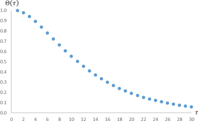
The reliability of a typical mortgage loan over time. A simulation of the reliability function $\mathrm{\Theta }\left(\tau \right)$ for a typical 30-year FRM loan (in Eq. (26)) with ${\alpha }_S=0.09$ as the systemic job market failure rate per year, ${\alpha }_I=0.02$ as the idiosyncratic job market failure rate per year, ${\alpha }_{\mathit{HM}}=0.01$ as the housing market failure rate per year, therefore $\psi =0.23$ and $\chi =0.12$, and we let the time to range in the interval $\tau \in \left\{0,,,1,,,2,,,\cdots ,,,30\right\}$ years

As expected, in light of the different failure rates that affect the various modes of operation, the reliability function starts from one (100% reliability at initiation in ${\mathit{MLS}}_0$ for the 30-year FRM loan), and it gradually decreases. This persistent and natural decline in reliability first takes a concave form (having relatively fast deterioration), but then a convex shape (with somewhat slower deterioration). As observed in this simulation, $\mathrm{\Theta }\left(\tau \right)$ will converge to zero when enough time has passed because of the property $\underset{\tau \to \infty }{\lim }\mathrm{\Theta }\left(\tau \right)=\underset{\tau \to \infty }{\lim }\left(2,e^{-\chi \tau },-,e^{-\psi \tau }\right)=0$.

We should mention at this point that the overall reliability of many 30-year FRM loans may deteriorate at slower paces or might reach higher final levels than our recreation, even over this elongated time interval of 30 years. Throughout the simulations here, we intentionally select rather exaggerated quantities for the input variables to demonstrate the full range of consequences and output parameters.

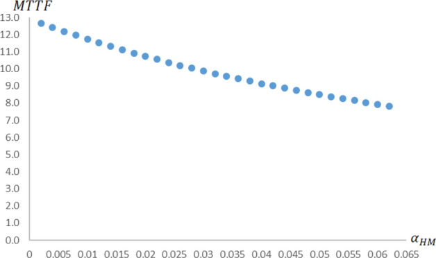
In Figs. 3, 4, and 5, we assess how the MTTF (in Eq. (27)) changes with respect to the systemic, idiosyncratic, and housing-market associated failure rates ${\alpha }_S$, ${\alpha }_I$, and ${\alpha }_{\mathit{HM}}$, respectively. In Fig. 3, we simulate the MTTF as a function of ${\alpha }_S$ by arbitrarily selecting ${\alpha }_S\in \left\{0.003,,,0.006,,,0.009,,,\cdots ,,,0.093\right\}$ as the systemic job market failure rates per year, ${\alpha }_I=0.026$ as the idiosyncratic job market failure rate per year, and ${\alpha }_{\mathit{HM}}=0.02$ as the housing market failure rate per year. In Fig. 4, we simulate the MTTF as a function of ${\alpha }_I$ by arbitrarily choosing ${\alpha }_S=0.068$ as the systemic job market failure rate per year, ${\alpha }_I\in \left\{0.001,,,0.004,,,0.007,,,\cdots ,,,0.091\right\}$ as the idiosyncratic job market failure rates per year, and ${\alpha }_{\mathit{HM}}=0.001$ as the housing market failure rate per year. In Fig. 5, we simulate the MTTF as a function of ${\alpha }_{\mathit{HM}}$ by arbitrarily picking ${\alpha }_S=0.08$ as the systemic job market failure rate per year, ${\alpha }_I=0.036$ as the idiosyncratic job market failure rate per year, and ${\alpha }_{\mathit{HM}}\in \left\{0.002,,,0.004,,,0.006,,,\cdots ,,,0.062\right\}$ as the housing market failure rates per year.

Fig. 3.

Mean time to failure as a function of the systemic risks in the job market. A simulation of the MTTF function for a typical 30-year FRM loan (in Eq. (27)) with ${\alpha }_S\in \left\{0.003,,,0.006,,,0.009,,,\cdots ,,,0.093\right\}$ as the systemic job market failure rates per year, ${\alpha }_I=0.026$ as the idiosyncratic job market failure rate per year, and ${\alpha }_{\mathit{HM}}=0.02$ as the housing market failure rate per year

Fig. 4.

Mean time to failure as a function of the idiosyncratic risks in the job market. A simulation of the MTTF function for a typical 30-year FRM loan (in Eq. (27)) with ${\alpha }_S=0.068$ as the systemic job market failure rate per year, ${\alpha }_I\in \left\{0.001,,,0.004,,,0.007,,,\cdots ,,,0.091\right\}$ as the idiosyncratic job market failure rates per year, and ${\alpha }_{\mathit{HM}}=0.001$ as the housing market failure rate per year

Fig. 5.

Mean time to failure as a function of the contractionary risks in the housing market. A simulation of the MTTF function for a typical 30-year FRM loan (in Eq. (27)) with ${\alpha }_S=0.08$ as the systemic job market failure rate per year, ${\alpha }_I=0.036$ as the idiosyncratic job market failure rate per year, and ${\alpha }_{\mathit{HM}}\in \left\{0.002,,,0.004,,,0.006,,,\cdots ,,,0.062\right\}$ as the housing market failure rates per year

In all of these three recreations, we notice that the MTTF tends to decrease at a decreasing rate (having singular convex patterns though) with the corresponding failure rates. However, we also detect that the specific risks that emerge from the housing market (communicated through ${\alpha }_{\mathit{HM}}$ in Fig. 5) convey the leading factor influencing the MTTF of a 30-year FRM loan. Throughout these three simulations, we alternate the failure rates along rather comparable quantities, yet ${\alpha }_{\mathit{HM}}$ is the failure rate that contracts the MTTF the most. This particular aftermath is a direct result of the inherent asymmetry in our model, where a failure in the housing market has no redundancy, as opposed to any type of failure in the job market.7 In essence, a failure in the housing market immediately leads to an absorbing state (in ${\mathit{MLS}}_3$, ${\mathit{MLS}}_4$, or ${\mathit{MLS}}_7$), though any single failure in the job market (both systemic and idiosyncratic) only leads to a higher-risk but still an operative state of nature (in ${\mathit{MLS}}_1$ or ${\mathit{MLS}}_2$). The 30-year FRM loan becomes delinquent with two successive failures in the job market (in ${\mathit{MLS}}_5$ or ${\mathit{MLS}}_6$).

In Fig. 6, we simulate the overall probability $P_S\left(\tau \right)$ that at least one spouse has lost his or her source of income in light of systemic risks in the job market over time with ${\alpha }_S=0.08$ as the systemic job market failure rate per year, ${\alpha }_I=0.02$ as the idiosyncratic job market failure rate per year, ${\alpha }_{\mathit{HM}}=0.01$ as the housing market failure rate per year, therefore $\psi =0.21$ and $\chi =0.11$ (both are constants here), and we let the time to progress in the relevant interval $\tau \in \left\{0,+,,,1,,,2,,,\cdots ,,,30\right\}$ years. As predicted by analytical derivation (28), this cumulative likelihood first increases (with concavity) but then decreases (with convexity) over time, reaching its highest simulated level of $P_S\left(\tau \right)\cong 0.405$ after seven years (according to Eq. (30) and the arbitrarily selected values in this simulation, ${\tau }^{\ast }\cong 7.282$). Over a long enough horizon, $P_S\left(\tau \right)$ in Eq. (28) will converge to its asymptote $\underset{\tau \to \infty }{\lim }{P}_S\left(\tau \right)=\frac{2{\alpha }_I+{\alpha }_{\mathit{HM}}}{\psi }+{2{\alpha }_I^2+2\alpha }_S{\alpha }_I$, which is about 0.242 here.

Fig. 6.

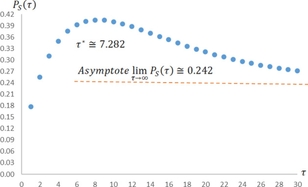
The overall probability that at least one person has lost his / her income because of the systemic risks in the job market over time. A simulation of the overall probability $P_S\left(\tau \right)$ that at least one of the spouses has lost his or her source of income because of systemic risks in the job market (in Eq. (28)) with ${\alpha }_S=0.08$ as the systemic job market failure rate per year, ${\alpha }_I=0.02$ as the idiosyncratic job market failure rate per year, ${\alpha }_{\mathit{HM}}=0.01$ as the housing market failure rate per year, therefore $\psi =0.21$ and $\chi =0.11$ (both are fixed here), and we let the time to progress in the interval $\tau \in \left\{0,+,,,1,,,2,,,\cdots ,,,30\right\}$ years. The simulated maximum probability is achieved at $\tau =7$ years (while analytically, from Eq. (30), ${\tau }^{\ast }\cong 7.282$), with $P_S\left(\tau \right)\cong 0.405$. Over a long enough horizon, $P_S\left(\tau \right)$ (in Eq. (28)) will converge to its asymptote $\underset{\tau \to \infty }{\lim }{P}_S\left(\tau \right)=\frac{2{\alpha }_I+{\alpha }_{\mathit{HM}}}{\psi }+{2{\alpha }_I^2+2\alpha }_S{\alpha }_I$, which is about 0.242 here

In Fig. 7, we simulate the overall probability $P_I\left(\tau \right)$ that at least one spouse has lost his or her source of income in light of idiosyncratic risks in the job market over time with ${\alpha }_S=0.035$ as the systemic job market failure rate per year, ${\alpha }_I=0.06$ as the idiosyncratic job market failure rate per year, ${\alpha }_{\mathit{HM}}=0.025$ as the housing market failure rate per year, therefore $\psi =0.215$ and $\chi =0.12$ (both are constants here), and we let the time to progress in the relevant interval $\tau \in \left\{0,+,,,1,,,2,,,\cdots ,,,30\right\}$ years. Similar to before, and as predicted by analytical derivation (31), this cumulative likelihood first increases (with concavity) but then decreases (with convexity) over time, reaching its highest simulated level of $P_I\left(\tau \right)\cong 0.685$ after eight years (according to Eq. (33) and the arbitrarily selected values in this simulation, ${\tau }^{\ast }\cong 7.513$). Over a long enough horizon, $P_I\left(\tau \right)$ in Eq. (31) will converge to its asymptote $\underset{\tau \to \infty }{\lim }{P}_I\left(\tau \right)=\frac{2{\alpha }_S+{\alpha }_{\mathit{HM}}}{\psi }+{2{\alpha }_S^2+2\alpha }_S{\alpha }_I$, which is roughly 0.449 in this case.

Fig. 7.

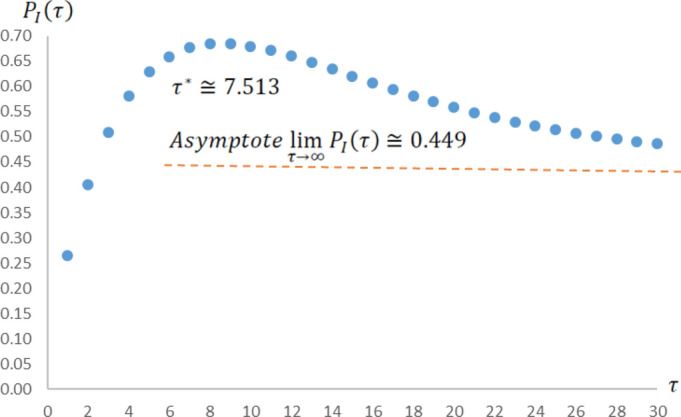
The overall probability that at least one person has lost his / her income because of the idiosyncratic risks in the job market over time. A simulation of the overall probability $P_I\left(\tau \right)$ that at least one of the spouses has lost his or her source of income because of idiosyncratic risks in the job market (in Eq. (31)) with ${\alpha }_S=0.035$ as the systemic job market failure rate per year, ${\alpha }_I=0.06$ as the idiosyncratic job market failure rate per year, ${\alpha }_{\mathit{HM}}=0.025$ as the housing market failure rate per year, therefore $\psi =0.215$ and $\chi =0.12$ (both are fixed here), and we let the time to progress in the interval $\tau \in \left\{0,+,,,1,,,2,,,\cdots ,,,30\right\}$ years. The simulated maximum probability is achieved at $\tau =8$ years (while analytically, from Eq. (33), ${\tau }^{\ast }\cong 7.513$), with $P_I\left(\tau \right)\cong 0.685$. Over a long enough horizon, $P_I\left(\tau \right)$ (in Eq. (31)) will converge to its asymptote $\underset{\tau \to \infty }{\lim }{P}_I\left(\tau \right)=\frac{2{\alpha }_S+{\alpha }_{\mathit{HM}}}{\psi }+{2{\alpha }_S^2+2\alpha }_S{\alpha }_I$, which is roughly 0.449 here

It is also worth mentioning here that the last two illustrations exhibit realistic setups with early upward but then downward sloping curves, because with relatively rare housing market rapid significant declines in practice, hence with fairly low ${\alpha }_{\mathit{HM}}$, the failure rates ${\alpha }_S$ and ${\alpha }_I$ often become dominant in the system. In this common scenarios, $P_S\left(\tau \right)=P_1\left(\tau \right)+P_3\left(\tau \right)+P_5\left(\tau \right)$ in Fig. 6 or $P_I\left(\tau \right)=P_2\left(\tau \right)+P_4\left(\tau \right)+P_6\left(\tau \right)$ in Fig. 7, respectively accumulate mounting odds at the beginning, i.e., they both grow at the expense of the likelihood to shift from ${\mathit{MLS}}_0$ to the absorbing ${\mathit{MLS}}_7$. Nonetheless, the ergodic properties of the model dictate that, unless the system has already reached any of the absorbing states (${\mathit{MLS}}_3$ and ${\mathit{MLS}}_5$ in Fig. 6 or ${\mathit{MLS}}_4$ and ${\mathit{MLS}}_6$ in Fig. 7), the cumulative probabilities $P_S\left(\tau \right)$ and $P_I\left(\tau \right)$ will start to decay over time, because of the growing chances to elude the transition states of nature (${\mathit{MLS}}_1$ in Fig. 6 and ${\mathit{MLS}}_2$ in Fig. 7) and move outside of the respective domains of $P_S\left(\tau \right)$ and $P_I\left(\tau \right)$, i.e., from ${\mathit{MLS}}_1$ to ${\mathit{MLS}}_6$ or from ${\mathit{MLS}}_2$ to ${\mathit{MLS}}_5$. In our distinct simulations, we aim the arbitrarily selected values for the transition rates to genuinely represent this realm. We occasionally inflate the chosen values (for rich sensitivity analyses) although with reasonable proportions.

Estimation Guidelines

To make the current model more tangible, we concisely discuss in this section some estimation guidelines and ongoing calibration practices for the model’s input variables. Our proposed compartmental model aims to be parsimonious, thus it is essentially assembled from only three input variables: ${\alpha }_S$ as the systemic job market failure rate per year, ${\alpha }_I$ as the idiosyncratic job market failure rate per year, and ${\alpha }_{\mathit{HM}}$ as the housing market failure rate per year. In practice, all three entries can be approximated and tuned over time to fit various economic conditions and personal circumstances from actuarial data, as explained hereafter.

Systemic failures in the job market could evolve from diverse macroeconomic disorders (or structural breaks in the economic status quo) including rising national or domestic unemployment rates, gradual transformations in employment opportunities (such as relocation of corporations and other employers from one state to another), global technological advances (such as computerization, automation, mechanization, etc.), ongoing trends in specific industries or subsectors (for example, major setbacks to airlines, tourism, and hospitality firms as the result of a spread of a pandemic, such as the COVID-19), and in our context also regulatory or policy changes that impact the particular jobs at which the mortgage loan borrowers are proficient and currently employed (for instance, certain energy or construction initiatives could be placed on hold by new administrations). There are in fact numerous governmental institutions and other independent agencies that publicly pursue the likelihoods for these proceedings.8 Thus, to remain vigilant, we recommend that lenders should not forecast ${\alpha }_S$ for the next 30 years or so, but roughly guesstimate ${\alpha }_S$ for the systemic risks in the underlying jobs and the relevant industries (to the mortgage loan borrowers) over a sensible horizon, and then adjust it over time.

Idiosyncratic (and not easily reversible) failures in the job market mainly arise because of deteriorating chronic health conditions and the lack of skills, training, education, personality, or motivation to continue working in a certain occupation. Insurance companies naturally hold actuarial (national and more geographically targeted) data on the rates at which both males and females in different age groups may develop symptoms for chronic diseases and consequently lose their jobs. The remaining personal merits involve soft information, and as such, they are more difficult to measure and quantify. Yet, some proxy variables (such as FICO scores or the level and specific concentration of higher education of the mortgage borrowers) could be used to assess these factors. Alternatively, a symbolic premium can be added for them to better approximate ${\alpha }_I$ for upcoming individuals that apply for mortgage loans. This premium can be assessed by reverse engineering the model, once all other input variables are introduced, and the outcome results are aligned with known records of job market and housing market failures.

For example, if the traditional maximum likelihood for idiosyncratic risks in the job market $P_I\left(\tau \right)$ is set as 0.40 per year, and the other two input variables are identified as ${\alpha }_S=0.02$ and ${\alpha }_{\mathit{HM}}=0.027$, then by solving backward Eq. (31) we can learn that ${\alpha }_I=0.085$. If, in addition, actuarial data shows that, historically, the average proportion of a certain population that develops chronic health conditions, which prevent one from doing his or her routine job tasks, is 0.05 per year, then we can deduce that the premium for the personal merits mentioned above should be 0.035 per year. In this case, 3.5% of a given population would lose their sources of income per year because of lack of skills, training, education, or sufficient motivation to continue working.9

In most developed countries, some data is also available concerning ${\alpha }_{\mathit{HM}}$, based on previous episodes of housing market severe downturns throughout modern history. Clearly, past events do not necessarily predict future happenings, but over the past decades, extensive empirical economic research has successfully identified and narrowed the key observable determinants and their coefficients for housing market calamities of various kinds.10 These accessible enquiries and methodologies can assist lenders in their search for the housing market failure rate ${\alpha }_{\mathit{HM}}$, which can be regularly updated as well.

Summary

In this study, we have developed and demonstrated a relatively simple risk model that accounts for the different states and hazard rates of a typical 30-year FRM loan. Our generic scheme accounts for two feasible modes of operation (active and delinquent) and three types of common risks to conventional mortgage loans (systemic risks and idiosyncratic risks within the job market, and the risk of a collapse in the housing market). We also consider that these popular mortgage loans are frequently undertaken by married couples with redundant sources of income (in the sense that they back up each other, and a single paycheck is sufficient to support the mortgage loan monthly payments), yet the ad hoc conditions of the housing market are independent of these employments. The proposed model aims to be parsimonious and universal, and therefore it could fit a large spectrum of economic conditions and personal circumstances.

Nevertheless, the current generic model can be modified and account for other (more or less complex) settings as well. It is beyond the scope of this study to derive all the formulations and recreate the sensitivity analyses for all these feasible scenarios, but we shall concisely discuss these alternatives here. Analogous schemes may further comprise only a single mortgage loan borrower. In that conventional case, the mortgagor has no income back up, thus the model would converge to only four states of nature, with ${\mathit{MLS}}_0$ as the initial active state, and ${\mathit{MLS}}_1$, ${\mathit{MLS}}_2$, and ${\mathit{MLS}}_7$ as the three immediate absorbing states stemming from systemic, idiosyncratic, and housing market risks, respectively.11 Other systems may embed rescindable states of nature. When instances of job loss are temporary, for example, the reliability model would include reverse transition rates from ${\mathit{MLS}}_1$ and ${\mathit{MLS}}_2$ back to ${\mathit{MLS}}_0$ (clearly with distinct values).

Other ordinary situations may comprise detached measures of systemic risks (because of different underlying occupations, which are associated with different employment environments, for instance) and idiosyncratic risks (because of different health conditions or other personal circumstances, for example) for the married couple. In this viable case, the two spouses face diverse hazards in the job market, and a modified model would distinguish between ${\alpha }_{I,1}$ and ${\alpha }_{I,2}$, and between ${\alpha }_{S,1}$ and ${\alpha }_{S,2}$, while it would also account for the chronological order of the transition rates. Another complication of the present model could consider that mortgagors do not always default upon a housing market crash, even when their house is in negative equity (or “under water”). This scenario would add new absorbing states with probabilities or transition rates that correspond to the new conditions.

The model can also incorporate higher resolution of the legal system (i.e., to consider not only prompt loans and delinquent loans, but also ultimate foreclosures. In this intricate setting, delinquent states of nature would become transient states, and foreclosure states of nature would be the absorbing states (different cost structures can be attributed to these separate states as well). In addition, other variations of the model may also include possible statistical dependency between the job market and the housing market (with mathematically correlated transition rates, i.e., ${\alpha }_S$ and ${\alpha }_{\mathit{HM}}$ can have a proportion coefficient that links them, which could also path a direct transition from ${\mathit{MLS}}_0$ to ${\mathit{MLS}}_3$). Simultaneous events such as where both spouses can lose their income sources together are possible as well. This setting fits circumstances where both spouses jointly work in a small family business, for example. Other models may also account for ARM loans that further contemplate interest rate and prepayment risks. As stated before, the current model does not aspire to capture all possible economic scenarios, but merely to serve as a preliminary framework for more variants. We thus recommended that intrigued researchers explore these alternative paths and form a set of generic models for the most common situations.

Data availability

This study presents a theoretical model and no data is used.

Declarations

Conflict of Interest

The author has no conflicts of interest and no funding to report.

References

- Alexander W, Grimshaw SD, McQuen GR, Slade BA. Some loans are more equal than others: Third-party originations and defaults in the subprime mortgage industry. Real Estate Economics. 2002;30(4):667–697. doi: 10.1111/1540-6229.t01-1-00054. [DOI] [Google Scholar]
- Ambrose BW, Capone CA. Cost-benefit analysis of single-family foreclosure alternatives. The Journal of Real Estate Finance and Economics. 1996;13:105–120. doi: 10.1007/BF00154051. [DOI] [Google Scholar]
- Ambrose BW, Capone CA. Modeling the conditional probability of foreclosure in the context of single-family mortgage default resolutions. Real Estate Economics. 1998;26(3):391–429. doi: 10.1111/1540-6229.00751. [DOI] [Google Scholar]
- Ambrose BW, Capone CA. The hazard rates of first and second defaults. The Journal of Real Estate Finance and Economics. 2000;20:275–293. doi: 10.1023/A:1007837225924. [DOI] [Google Scholar]
- Aron J, Muellbauer J. Modelling and forecasting mortgage delinquency and foreclosure in the UK. Journal of Urban Economics. 2006;94:32–53. doi: 10.1016/j.jue.2016.03.005. [DOI] [Google Scholar]
- Balagurusamy E. Reliability Engineering. McGraw-Hill; 1984. [Google Scholar]
- Beem RH. Residential mortgage delinquency rates: The determinants of default. Issues in Political Economy. 2014;23:59–75. [Google Scholar]
- Calem P, Cillen K, Wachter S. The neighborhood distribution of subprime mortgage lending. The Journal of Real Estate Finance and Economics. 2004;29:393–410. doi: 10.1023/B:REAL.0000044020.67401.51. [DOI] [Google Scholar]
- Calem P, Wachter S. Community reinvestment and credit risk: Evidence from affordable-home-loan program. Real Estate Economics. 1999;27:105–134. doi: 10.1111/1540-6229.00768. [DOI] [Google Scholar]
- Campbell TS, Dietrich JK. The determinants of default on insured conventional residential mortgage loans. The Journal of Finance. 1983;38(5):1569–1581. doi: 10.2307/2327587. [DOI] [Google Scholar]
- Capozza DR, Thomson TA. Optimal stopping and losses on subprime mortgages. The Journal of Real Estate Finance and Economics. 2005;30(2):115–131. doi: 10.1007/s11146-004-4875-z. [DOI] [Google Scholar]
- Capozza DR, Thomson TA. Subprime transitions: Lingering and malingering in default? The Journal of Real Estate Finance and Economics. 2006;33(3):241–258. doi: 10.1007/s11146-006-9984-4. [DOI] [Google Scholar]
- Chicone C. Ordinary differential equations with applications. 2. Cham: Springer; 2000. [Google Scholar]
- Chinloy P. Privatized default risk and real estate recessions: The U.K. mortgage market. Real Estate Economics. 1995;23:410–420. doi: 10.1111/1540-6229.00672. [DOI] [Google Scholar]
- Coddington EA, Levinson N. Theory of Ordinary Differential Equations. McGraw-Hill; 1955. [Google Scholar]
- Courchane M, Surette B, Zorn P. Subprime borrowers: Mortgage transitions and outcomes. The Journal of Real Estate Finance and Economics. 2004;29:365–392. doi: 10.1023/B:REAL.0000044019.57580.18. [DOI] [Google Scholar]
- Cowan A, Cowan C. Default correlation: An empirical investigation of a subprime lender. Journal of Banking and Finance. 2004;28(4):753–771. doi: 10.1016/j.jbankfin.2003.10.005. [DOI] [Google Scholar]
- Cutts AC, van Order RA. On the economics of subprime lending. The Journal of Real Estate Finance and Economics. 2005;30(2):167–196. doi: 10.1007/s11146-004-4878-9. [DOI] [Google Scholar]
- Danis MA, Pennington-Cross A. A dynamic look at subprime loan performance. The Journal of Fixed Income. 2005;15(1):28–39. doi: 10.3905/jfi.2005.523088. [DOI] [Google Scholar]
- Demyanyk Y, Hemert OV. Understanding the subprime mortgage crisis. Review of Financial Studies. 2011;24(6):1848–1880. doi: 10.1093/rfs/hhp033. [DOI] [Google Scholar]
- Doms M, Furlong F, Krainer J. House prices and subprime mortgage delinquencies. Federal Reserve Bank of San Francisco Economic Letter. 2007;14(June):1–3. [Google Scholar]
- Doms, M., F. Furlong, and J. Krainer. 2007b. Subprime mortgage delinquency Rates. Working Paper, Federal Reserve Bank of San Francisco, 2007-33.
- Foote CL, Gerardi K, Willen PS. Negative equity and foreclosure: Theory and evidence. Journal of Urban Economics. 2008;64(2):234–245. doi: 10.1016/j.jue.2008.07.006. [DOI] [Google Scholar]
- Foote CL, Goette L, Willen PS. Just the facts: An initial analysis of the subprime crisis. Journal of Housing Economics. 2008;17(4):291–305. doi: 10.1016/j.jhe.2008.09.005. [DOI] [Google Scholar]
- Jiang W, Nelson AA, Vytlacil E. Delinquency model predictive power among low-documentation loans. Economics Letters. 2013;120(2):171–173. doi: 10.1016/j.econlet.2013.03.046. [DOI] [Google Scholar]
- Jiang W, Nelson AA, Vytlacil E. Mortgage securitization and loan performance: A contrast of ex ante and ex post relations. Review of Financial Studies. 2013;27(2):454–483. doi: 10.1093/rfs/hht073. [DOI] [Google Scholar]
- Jiang W, Nelson AA, Vytlacil E. Liar’s loan? Effects of origination channel and information falsification on mortgage delinquency. The Review of Economics and Statistics. 2014;96(1):1–18. doi: 10.1162/REST_a_00387. [DOI] [Google Scholar]
- Kaufmann RK, Gonzalez N, Nickerson TA, Nesbit TS. Do household energy expenditures affect mortgage delinquency rates? Energy Economics. 2011;33(2):188–194. doi: 10.1016/j.eneco.2010.07.007. [DOI] [Google Scholar]
- Keys BJ, Mukherjee T, Seru A, Vig V. Did securitization lead to lax screening? Evidence from subprime loans. Quarterly Journal of Economics. 2010;125(1):307–362. doi: 10.1162/qjec.2010.125.1.307. [DOI] [Google Scholar]
- Keys, B.J., T. Piskorski, A., Seru, and V. Yao V. 2014. Mortgage rates, household balance sheets, and the real economy. NBER Working Paper, No. 20561 (October).
- Kumar KC, Lamberson LR. Reliability in Engineering Design. John Wiley & Sons Inc; 1977. [Google Scholar]
- Lin Z, Liu Y, Jia X. Immigrants and mortgage delinquency. Real Estate Economics. 2016;44(1):198–235. doi: 10.1111/1540-6229.12092. [DOI] [Google Scholar]
- Mayer C, Pence K, Sherlund S. The rise in mortgage defaults: Facts and myths. Journal of Economic Perspectives. 2009;23(1):27–50. doi: 10.1257/jep.23.1.27. [DOI] [Google Scholar]
- Mian A, Sufi A. The consequences of mortgage credit expansion: Evidence from the US mortgage default crisis. The Quarterly Journal of Economics. 2009;124(4):1449–1496. doi: 10.1162/qjec.2009.124.4.1449. [DOI] [Google Scholar]
- Morton TG. A discriminant function analysis of residential mortgage delinquency and foreclosure. Real Estate Economics. 1975;3(1):73–88. doi: 10.1111/1540-6229.00133. [DOI] [Google Scholar]
- Parnes D. Abnormal mortgage delinquencies as housing crisis early symptoms. International Journal of Housing Markets and Analysis. 2018;11(2):412–432. doi: 10.1108/IJHMA-05-2017-0055. [DOI] [Google Scholar]
- Pennington-Cross A. Subprime lending in the primary and secondary markets. Journal of Housing Research. 2002;13(1):31–50. [Google Scholar]
- Pennington-Cross A. Credit history and the performance of prime and nonprime mortgages. The Journal of Real Estate Finance and Economics. 2003;27:279–301. doi: 10.1023/A:1025891223226. [DOI] [Google Scholar]
- Pennington-Cross A, Chomsisengphet S. Subprime refinancing: Equity extraction and mortgage termination. Real Estate Economics. 2007;35(2):233–263. doi: 10.1111/j.1540-6229.2007.00189.x. [DOI] [Google Scholar]
- Quercia RG, Stegman MA. Residential mortgage default: A review of the literature. Journal of Housing Research. 1992;3(2):341–379. [Google Scholar]
- Vandell KD, Thibodeau T. Estimation of mortgage defaults using disaggregate loan history data. Real Estate Economics. 1985;13(3):292–316. doi: 10.1111/1540-6229.00356. [DOI] [Google Scholar]
- von Furstenberg GM, Green RJ. Estimation of delinquency risk for home mortgage portfolios. Real Estate Economics. 1974;2(1):5–19. doi: 10.1111/1540-6229.00117. [DOI] [Google Scholar]
- von Furstenberg GM, Green RJ. Home mortgage delinquencies: A cohort analysis. The Journal of Finance. 1974;29(5):1545–1548. doi: 10.2307/2978558. [DOI] [Google Scholar]
- Webb BG. Borrower risk under alternative mortgage instruments. The Journal of Finance. 1982;37(1):169–183. doi: 10.2307/2327124. [DOI] [Google Scholar]
Associated Data
This section collects any data citations, data availability statements, or supplementary materials included in this article.
Data Availability Statement