An Integrated Approach of Learning Genetic Networks From Genome-Wide Gene Expression Data Using Gaussian Graphical Model and Monte Carlo Method

Abstract

Global genetic networks provide additional information for the analysis of human diseases, beyond the traditional analysis that focuses on single genes or local networks. The Gaussian graphical model (GGM) is widely applied to learn genetic networks because it defines an undirected graph decoding the conditional dependence between genes. Many algorithms based on the GGM have been proposed for learning genetic network structures. Because the number of gene variables is typically far more than the number of samples collected, and a real genetic network is typically sparse, the graphical lasso implementation of GGM becomes a popular tool for inferring the conditional interdependence among genes. However, graphical lasso, although showing good performance in low dimensional data sets, is computationally expensive and inefficient or even unable to work directly on genome-wide gene expression data sets. In this study, the method of Monte Carlo Gaussian graphical model (MCGGM) was proposed to learn global genetic networks of genes. This method uses a Monte Carlo approach to sample subnetworks from genome-wide gene expression data and graphical lasso to learn the structures of the subnetworks. The learned subnetworks are then integrated to approximate a global genetic network. The proposed method was evaluated with a relatively small real data set of RNA-seq expression levels. The results indicate the proposed method shows a strong ability of decoding the interactions with high conditional dependences among genes. The method was then applied to genome-wide data sets of RNA-seq expression levels. The gene interactions with high interdependence from the estimated global networks show that most of the predicted gene-gene interactions have been reported in the literatures playing important roles in different human cancers. Also, the results validate the ability and reliability of the proposed method to identify high conditional dependences among genes in large-scale data sets.

Introduction

The estimation of gene regulatory networks is the reverse engineering for inferring network structures from different gene expressed products such as transcribed RNA or translated proteins.¹ Many approaches in previous studies were proposed for learning gene regulatory networks. Bayesian networks (BNs) reveal directed acyclic graph structures of networks, in which nodes represent random variables and directed edges indicate causal probabilistic conditional independencies,² and therefore, they have often been applied to gene expression data for inferring causal gene regulatory networks.^3-6 Considering the fact that BNs are unable to reflect feedback loops existing in real biological networks, the dynamic Bayesian networks were proposed and applied to gene expression data for inferring causal interaction relationship of genes.^7-10 However, the primary practical problem with the BNs is their computational complexity. It has been demonstrated that learning BNs from data is an NP-complete problem. Algorithms for learning BNs from data include 2 main components: a scoring metric and a search procedure. The search procedure is used to identify network with high scores, and the article by Chickering¹¹ shows that the search problem of identifying a BN is NP-complete. However, simple correlation matrices have been applied in several fields for analyzing the correlation of variables and used as another instrument to extract correlation patterns between genes that are presented in gene expression data.¹² Many researchers have proposed using correlation matrices for the analysis of gene interaction networks.^13-19

The Gaussian graphical models (GGMs), unlike BNs, define undirected graph structures of networks that represent the conditional dependence between variables. The GGM has been widely applied to gene expression data for analyzing gene interactions. Several techniques were reported for GGM model parameter selection; among them are the standard greedy stepwise forward selection^20,21 and the improved model selection approach.²² Using the fact that a gene regulatory network is typically sparse, a lasso-based method²³ was introduced to improve the accuracy by shrinking the nonzero values that might just be noise in the precision matrix representing a GGM. An increasing number of algorithms have since been proposed to estimate the precision matrix, such as gradient directed regularization for sparse Gaussian concentration graphs,²⁴ neighborhood selection with the Lasso,²⁵ the penalized likelihood method,^26,27 the stability approach to regularization selection for GGM,²⁸ the novel Bayesian method for building the GGMs,^29,30 and the joint graphical lasso.³¹ However, these algorithms for analyzing gene interactions focus on relatively small data sets that include a small part of the genes. As a result, some potentially highly significant gene interactions in a large-scale study could be omitted by those small-scale algorithms. Also, these approaches are computationally costly, making them ineffective to be applied to large data sets, such as genome-wide gene expression data sets. Other recent methods on inference of GGM are as follows: an integrated statistical framework based on the graph lasso which is applied to learning gene networks under single-nucleotide-polymorphism perturbations using eQTL data sets was developed.³² A novel regression-based method was proposed to obtain asymptotically normal estimation of a large GGM,³³ and it provides both P values and confidence intervals for each edge in the graph. Based on the penalized likelihood inference, a bias correction approach was applied to make inference of each edge.³⁴ A high-dimensional inference of Gaussian copula graphical model³⁵ was developed based on a novel decorrelated score test statistic.³⁶ A bottom-up GGM algorithm was developed for constructing multilayered hierarchical gene regulatory network on RNA-seq data sets.³⁷ However, these methods also encounter expensive computation issue when they are applied in real biological application.

In this study, an effective network learning model that integrates traditional GGM with the Monte Carlo method (MCGGM) was developed for learning a global network from genome-wide gene expression data. Monte Carlo Gaussian graphical model was applied and verified on a relatively small, real data set of RNA-seq gene expression levels, and the estimated results indicate its strong ability of identifying the interactions with high conditional dependences. Monte Carlo Gaussian graphical model was then applied to a genome-wide data set of RNA-seq gene expression levels. The results validate the ability and reliability of the approach in identifying strong conditional dependences among genes. The contributions of this study are (1) the proposed MCGGM algorithm speeds up the GGM in estimation of large-scale data set and makes it feasible to infer genetic networks under the framework of GGM at a genome-wide scale and (2) the estimated interactions in genome-wide expression data sets provide insights for biologists to explore the complicated molecular interactions.

Model and Methods

A GGM is characterized through the precision matrix, rather than the covariance matrix, of the random variables involved.

Given gene expression data $Y={[y_1,\dots y_n]}^T\in R^{n\times p}$ for $n$ samples and $p$ genes, the gene expression profile of each sample, $y_i={[y_i^1,\dots y_i^p]}^T$ , is assumed to be independent and follows a Gaussian distribution $N(u,\Sigma ),$ where $u$ is the mean and $\Sigma$ is the $p\times p$ covariance matrix. The precision matrix $\Theta ={\Sigma }^{-1}$ is a positive definite and symmetric matrix and presents a model for an undirected graph $\mathrm{G}=(\mathrm{V},\mathrm{E})$ , where V is a set of $p$ vertices corresponding to the $p$ genes and the edge set $\mathrm{E}=\left\{e_{i,j}\right\}$ describes the conditional dependences among the $p$ genes. $e_{i,j}\ne 0$ indicates that gene $i$ and gene $j$ are conditionally dependent, whereas $e_{i,j}=0$ states the 2 genes $i$ and $j$ are conditionally independent of each other, given all other genes. Each entry ${\theta }_{i,j}$ of the precision matrix signifies the strength of the dependence relation. Therefore, learning genetic network is equivalent to estimating the precision matrix, ie, to maximize the log-likelihood with $L_1$ norm penalty on its precision matrix

$$\log \det (\Theta )-\mathrm{trace}\left(\mathrm{S}\Theta \right)-\rho {\Vert \Theta \Vert }_1$$ (1)

where S is the sample covariance matrix, $\rho$ is a non-negative penalty parameter which controls the sparsity of the inverse covariance matrix $\Theta$ and $\left|\right|\Theta |{|}_1={\sum }_i{\sum }_j\left|\theta {}_{i,j}\right|$ represent the $L_1$ norm of $\Theta$ .^27,38 Clearly, the larger the parameter $\rho$ is, the sparser the estimated $\rho$ would be. If $\rho =0$ , this problem is reduced to the typically maximum likelihood estimation problem, whereas when $\rho \to \infty$ , $\Theta =0$ regardless of what sample data sets are used in estimation.

To apply graphical lasso to infer the graphical model, 1 important issue is to choose the optimal penalty parameter $\rho$ , which controls the sparsity level of the estimated $\Theta$ and ensures its stability. Any network to be learned from experimental data could unavoidably include some irrelevant and unexpected interactions resulting from the intrinsic “noise” in the experimental data. An estimated network is expected to be robust with respect to different sample data. Therefore, models with some degree of stability require $\rho$ to be at a level so that the “noisy” edges in the estimated precision matrix are filtered out. Furthermore, genetic networks are typically considered to be sparse,³⁹ and therefore, the estimated network is expected to be sparse as well. To select an optimal value of the penalty parameter $\rho$ , the subsampling-based approach²⁸ was implemented and tested in this study.

The Monte Carlo method (MC) refers to a series of statistical methods that are essentially used to find solutions to computationally expensive problems.^40,41 The core of this method is to use stochastic sampling techniques to solve intractable problems that are too complicated to deal with analytically.⁴² The Monte Carlo method typically includes 2 major components: (1) random sampling and estimation and (2) estimation integration. Random sampling is used to run an estimation, and the estimates from multiple runs will then be integrated to improve the estimation. This technique has been used in developing algorithms for solving different problems in multiple fields, including computational biology,⁴³ applied statistics,⁴⁴ and artificial intelligence.⁴⁵ All the algorithms with MC share the concept of using random sampling to compute a solution to a given problem.⁴⁶

An integrated approach that uses the Monte Carlo random sampling technique is introduced to obtain large-scale GGMs. First, the large set of genes is randomly divided into subsets of equal size. In this way, the large data set is divided into multiple small subsets, making it feasible to directly apply the Gaussian graphical lasso to those subsets for analyzing gene-gene relationships. However, if a large set of genes is simply divided and estimated like this, only some isolated subnetworks are obtained. Some strong gene interactions that connect the subnetworks could be omitted and go undetected. To increase the probability of each gene pair having an opportunity to be sampled in the same subset, the process of random sampling (with replacement) and estimation in the first step will be repeated. Researchers expect that each pair of genes has some opportunity to be in the same subset so that the dependence of each pair of genes may be estimated. Monte Carlo Gaussian graphical model sets a threshold to terminate the iterations when the probability of any pair of genes not being sampled in at least 1 subset is less than or equal to the threshold. The estimated subnetworks are then integrated into a larger network that includes all genes under consideration. During the iterations, each random sampling is tracked and the number of pairs of genes sampled in a subset is recorded in a matrix. Each estimated subnetwork along with the edge weight corresponding to each pair of genes is recorded. The average edge weight of a pair of genes is considered the estimated strength of their dependency. Owing to noise in the data as well as sampling and rounding errors, it is inevitable that there are “noisy” values in the estimates. Because the focus is on finding those genes that are highly conditionally dependent, edges with small weights are filtered if the weights are less than a threshold calculated based on the SD of the edge weights or less than a threshold calculated based on the estimated global network.

Figure 1 illustrates the flowchart of MCGGM. Considering a gene to be a random variable, let $V=\{y^1,y^2,y^3,\dots ,y^q\}$ represent a set of $q$ random variables. The undirected graph $G=(V,E),$ where $E\subseteq V\times V$ represents the relationship between the variables and depicts the dependences of the random variables. For genetic networks, the number of genes/variables under consideration could be in the order of 2000, making the direct estimation of $E$ using the graphical lasso inefficient or even infeasible. The MCGGM approach deploys the divide-and-conquer strategy through the use of stochastic sampling, the steps being as follows:

Figure 1.

Flowchart of the proposed MCGGM approach for learning global genetic networks on genome-wide gene expression data set. GGM indicates Gaussian graphical model; MCGGM, Monte Carlo Gaussian graphical model.

1. Randomly partition $V$ into $n$ subsets with equal number of $b=q/n$ genes $(V=\left\{V_{11},V_{21},V_{31},\dots ,V_{n1}\right\})$ . Then, extract RNA-seq gene expression data $S_{i1}$ for genes in subset $V_{i1}=\{y^{i{1}_1},y^{i{1}_2},y^{i{1}_3},\dots ,y^{i{1}_b}\}$ , $i=1,\dots ,n$ . $S_{i1}=\{y_1^{i1},y_2^{i1},y_3^{i1},\dots ,y_j^{i1}\},j=1,\dots ,r$ . $y_j^{i1}=\{y_j^{i{1}_1},y_j^{i{1}_2},y_j^{i{1}_3},\dots ,y_j^{i{1}_b}\}$ represents the expression levels of genes of the patient $j$ in the sample of $r$ patients. The Gaussian graphical lasso is used to learn the dependences among the genes from $S_{i1}$ to obtain an estimate of the network ${\widehat{E}}_{i1}$ of the genes in $V_{i1}.$ The first-round approximation of the network structure/edge matrix ${\widehat{E}}_1$ can then be obtained by finding the union of the $n$ estimated subnetworks:

$${\widehat{E}}_1=\underset{i=1}{\overset{n}{\cup }}{\widehat{E}}_{i1}$$

• 2. Repeat step 1 $m$ times to obtain a sequence of approximations of $E$ , ${\widehat{E}}_1,{\widehat{E}}_2,{\widehat{E}}_3,\dots ,{\widehat{E}}_m$ .

• 3. Each ${\widehat{E}}_i$ is processed to remove weak connections. A threshold of 3 SDs is used to remove the edges whose weights are 3 SDs below the mean.

• 4. Obtain the final estimated edge matrix by integrating the m estimates:

$$\overline{E}=\sum _{i=1}^m{\widehat{E}}_i./N=({\overline{e}}_{kl})=\left(\sum _{i=1}^m\frac{{\widehat{e}}_{kl}^i}{n_{kl}}\right)$$

• where $N$ is a matrix in which each entry $n_{kl}=\max \{1,$ number of times gene $k$ and gene $l$ are in 1 subset during the $m$ round of partitions} and ./ is the right-array division operator that divides each element of the first operant by the corresponding element of the second operant.

• 5. The last step of noise reduction is applied to $\overline{E}$ in which an entry that is 3 SDs below the mean is filtered out.

To ensure a high confidence of the integrated network, the number of sampling rounds $m$ was selected based on a threshold $t$ so that the probability that a pair of genes is not in any subset during the $m$ rounds is bounded by $t$

$${\left(\frac{n-1}{n}\right)}^m\le t$$

In this study, $t=0.01,\mathrm{and}m$ is chosen to be $\lceil \frac{\lg (t)}{\lg (n-1)/n}\rceil$ where ⌈ ⌉ represents the ceiling function.

Results and Analysis

Results on the small data set

The integrated model MCGGM was tested and verified using 2 RNA-seq gene expression data sets. The first one is a small gene expression data set. The genes of the data set were collected from the common genes in 15 types of specific cancer pathway maps from the Kyoto Encyclopedia of Genes and Genomes (KEGG).⁴⁷ The RNA-seq expression levels of the genes were retrieved from The Cancer Genome Atlas (TCGA).⁴⁸ The data set of RNA-seq expression level was cleaned in 2 steps: (1) removal of the genes whose expression levels are zeros across all samples. It is possible that these genes did express but their levels were so low and were not picked up by RNA-seq technology. (2) Transformation of the expression data with log function. All 0s in the data set were replaced with 1s before transformation. Eventually, a cleaned data matrix that includes 515 samples and 430 genes was obtained. Both traditional GGM and MCGGM were then applied to the data set to obtain 2 edge matrices $E_{GGM}$ and $E_{MCGGM}$ . Let $E_{GGM}$ represent the actual genetic network and $E_{MCGGM}$ represent the estimated one, and the 2 matrices were compared and analyzed with a variety of metrics.

Analysis with confusion matrix and Jaccard coefficient

Confusion matrix and receiver operating characteristics (ROC) are useful tools to organize and visualize the performance of classifiers.⁴⁹ In this study, nonzero values in an edge matrix are classified as positive and zero values as negative. An ROC curve was constructed to choose an appropriate threshold to filter the noise in the estimated edge matrix. Nonzero values in the estimated matrix represent edges in the corresponding undirected graph, indicating potential interactions in the gene interaction network; however, it does not mean that all the estimated nonzero values indicate actual gene interactions. Some nonzero values in the estimated matrix might be noise called false positives (FPs). Inevitably, some noises (FPs) are present in the estimated gene interaction network. To find a tradeoff threshold so that the estimated matrix includes the true positives (TPs) as much as possible and the FPs as little as possible, the mean and corresponding SD of the nonzero values in the estimated edge matrix were computed. In the estimated edge matrix, most estimated values fall in the range between the value (mean − 3*SD) and the value (mean + 3*SD). The term (mean − 3*SD) represents the difference between the mean value and 3-time SD, and the term (mean + 3*SD) is the sum between the mean value and 3-time SD. To filter the small nonzero values, the values mean − 3*SD, mean − 2*SD, mean − SD, and mean were chosen as thresholds, and based on the estimated results, other discrete values 0.1, 0.08, 0.06, 0.04,0.02, and 0.01 were also chosen as thresholds to observe how the corresponding true positive rates (TPRs) and false positive rates (FPRs) change. The estimated matrix is expected to include more TPs and fewer FPs; the expected threshold is the one with a high TPR and a relatively low FPR in the ROC curve.

With the threshold list (0.1, 0.08, 0.06, 0.04, 0.02, 0.01, mean, mean − SD, mean − 2*SD, mean − 3*SD), the ROC curve reflecting the ratio of TPR and FPR of the thresholds is given in Figure 2 below. The red curve in Figure 2A reflects the performance of the MCGGM. To clearly observe the close markers in the red ROC curve, the markers in Figure 2A are enlarged and the last 4 marks are highlighted with different color strips in Figure 2B. From Figure 2B, clearly, the threshold (mean − 3*SD) indicates a high TPR, and therefore, it was selected to filter the noises in the estimated networks.

Figure 2.

(A) ROC curve with different thresholds in the estimated networks. The red curve reflects the performance of the MCGGM. The blue dash line represents the no skill ROC. (B) Zoom-in view of the ROC curve in (A) for FPR < 0.06. The different color strips indicate the corresponding thresholds shown in the top left corner in (B). FPR indicates false positive rate; MCGGM, Monte Carlo Gaussian graphical model; ROC, receiver operating characteristics; TPR, true positive rate.

Unlike TPR, which only focuses on the ratio of correctly identified gene interactions and all actual interactions, Jaccard coefficient⁵⁰ takes FPs into account to measure the performance of MCGGM. To focus on the interactions indicating strong conditional dependence, the edge matrices $E_{GGM}$ and $E_{MCGGM}$ were sorted in the descending order, and their TPR and Jaccard coefficient corresponding to different top percentages of the edges in the 2 matrices were compared and analyzed. The results are shown in Table 1.

Table 1.

The estimated TPR and Jaccard coefficient with different proportion of edges.

Top % of edges	$\left|E_{GGM}\right|$	$\left|E_{MCGGM}\right|$	$T{P}^a$	$TP{R}^b$ (%)	$FP{R}^c$ (%)	$TN{R}^d$ (%)	$J{(E_{GGM},E_{MCGGM})}^e$ (%)
100	4149	9171	4074	98.19	5.79	94.21	44.06
80	3319	7337	3260	98.22	4.59	95.41	44.08
60	2489	5503	2441	98.07	3.41	96.59	43.97
40	1660	3668	1624	97.83	2.26	97.74	43.84
20	830	1834	814	98.07	1.12	98.88	44.00

^aTP: true positive—if the value of the interaction is positive (nonzero) in $E_{GGM}$ and is also estimated as positive in $E_{MCGGM}$ .

^bTPR: true-positive rate =  $TP/totalpositivesin{E}_{GGM}$ .

^cFPR: false-positive rate =  $FP/totalnegativesin{E}_{GGM}$ .

^dTNR: true-negative rate =  $TN/totalnegativesin{E}_{GGM}$ .

^e $J(E_{GGM},E_{MCGGM})$ : $\left|E_{GGM}{\cap }^{}{E}_{MCGGM}\right|/\left|E_{GGM}{\cup }^{}{E}_{MCGGM}\right|$ .

From Table 1, first, the MCGGM method correctly identified 4074 edges of all the 4149 edges in $E_{GGM}$ ; the TPR is up to 98%. The TPR corresponding to other percentages of edges also shows high and stable values of TPR (around 98%). These stable TPR values show that the MCGGM method has strong ability of correctly identifying gene interactions. Second, lower FPR and higher TNR indicate that MCGGM also has strong probability of correctly identifying those gene pairs without probabilistic dependences. Third, their Jaccard coefficients show lower values (around 0.44). Comparing TPR and Jaccard coefficient, the major factor resulting in higher TPR, but a lower Jaccard coefficient, is that FPs are present in the formula for the Jaccard coefficient. In fact, there is a tradeoff: FPs are allowed to exist in the estimated networks; however, at the same time, more TPs and fewer FPs are expected in the estimated networks so that the real interactions will not be buried in massive number of FPs. Based on the evaluated results, considering the lower FPR shown in Figure 2, MCGGM has shown a good performance in learning gene interaction networks.

Analysis with correlation coefficient of strong gene interactions in $E_{GGM}$ and $E_{MCGGM}$

A stronger indicator of the MCGGM approaching the ground truth is the agreement between the ranks of the strong interactions in $E_{GGM}$ and their corresponding ranks in $E_{MCGGM}$ , that is, if an interaction is strong and has a high rank in $E_{GGM}$ , this interaction should also have a relatively high rank in the $E_{MCGGM}$ . To assess whether the interaction ranks are consistent between the actual network and estimated network, the correlation of edge weights in $E_{GGM}$ and $E_{MCGGM}$ was examined. The edges in $E_{GGM}$ are first sorted in the descending order of their weights, and their ranks of the corresponding interactions in $E_{MCGGM}$ are identified. The correlation coefficients of the top-ranked interactions are then calculated. Let $i$ represent the rank of an interaction in $E_{GGM}$ and $y_i$ represent the rank of this interaction in $E_{MCGGM}$ and consider the top t interactions $X_t$ from $E_{GGM}$ and their corresponding ranks $Y_t$ from $E_{MCGGM}$

$$X_t=\left\{1,\dots ,i,\dots t\right\}1\le i\le t\mathrm{and}{Y}_t=\left\{y_1,\dots ,y_i,\dots y_t\right\}$$

The correlation $r_t$ reflects the consistency of the ranks of these targeted common interactions in the $E_{GGM}$ and $E_{MCGGM}$ . If they have completely consistent ranks in both $E_{GGM}$ and $E_{MCGGM}$ , the corresponding $r_t$ should be equal to 1. In contrast, if they have completely reverse ranks, $r_t$ will be equal to −1. A value between 1 and −1 but closer to 1 reflects consistency between the ranks of the common interactions in the actual and estimated networks. Figure 3 illustrates how the correlation coefficients change with the increasing number of top interactions. The curve in Figure 3 sharply rises to the position corresponding to about 0.75 and keeps relatively stable with the increasing numbers of interactions. The result indicates that the identified interactions have relatively consistent and stable ranks in both $E_{GGM}$ and $E_{MCGGM}$ . That is, the networks estimated by traditional GGM and MCGGM have high consistency in identifying those strong gene-gene interactions.

Figure 3.

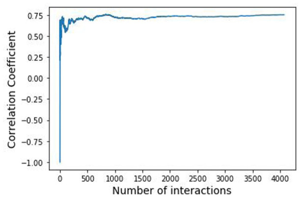
Correlation coefficient analysis of gene interactions in $E_{GGM}$ and $E_{MCGGM}$ . The horizontal axis denotes the number of common gene interactions in $E_{GGM}$ and $E_{MCGGM}$ and the vertical axis indicates the correlation coefficient $r_t$ .

Analysis of the missing strong gene interactions in $E_{MCGGM}$

Owing to the nature of the random sampling involved in MCGGM, it cannot be guaranteed that all pairs of interacting genes are sampled in a subset. Therefore, this leaves the possibility that some gene pairs might be strongly conditionally dependent in $E_{GGM}$ but cannot be identified in $E_{MCGGM}$ . To explore the probability of those interactions, the top 100 to 500 edges, respectively, from the sorted $E_{GGM}$ were extracted to examine whether these interactions were identified in $E_{MCGGM}$ . The results are shown in Table 2.

Table 2.

Identify the missing gene interactions in $E_{MCGGM}$ .

Top edges in $E_{GGM}$	All edges in $E_{MCGGM}$	Common edges	Number of missing edges
100	9171	98	2
200	9171	197	3
300	9171	296	4
400	9171	394	6
500	9171	494	6

Table 2 shows that a total of 6 among the top 500 interactions in $E_{GGM}$ were missing in $E_{MCGGM}$ . To intuitively compare these missing interactions, $E_{GGM}$ and $E_{MCGGM}$ were visualized in Figure 4A and B, respectively.

Figure 4.

Comparison of the interactions of missing gene pairs. (A) The interactions of missing gene pairs in $E_{GGM}$ . (B) The interactions of missing gene pairs in $E_{MCGGM}$ .

For the sake of easy and clear observation, these gene pairs and their interactions were magnified and marked with different colors. Obviously, the direct interactions between gene pairs PLCG2 and FLT3, PDGFB and NOTCH4, SHH and GLI1, E2F2 and CCNA2, SHH and E2F3, and PGR and BIRC5 of $E_{GGM}$ in Figure 4A were not identified in the estimated $E_{MCGGM}$ in Figure 4B.

To further explore a reasonable explanation why those direct interactions are not identified in $E_{MCGGM}$ , the sampled matrix N that tracks and records the number of gene pairs sampled in a subset through all the trials is examined. The value 0s for those gene pairs in the matrix $N$ indicate that those gene pairs are never sampled in a subset through all the trials. This is why their direct interactions could not be found in $E_{MCGGM}$ . However, in Figure 4B, although direct interactions are missing, their indirect interaction relationships through other genes in the shortest paths still can be found.

The aforementioned analysis results indicate the following facts. First, the proposed MCGGM has a strong ability of and high reliability in correctly identifying gene interactions, especially for strong conditional dependences. Second, there is a small probability that few direct interactions of gene pairs might not be identified because they were never sampled in 1 group during the estimation process. However, this possibility has an acceptable probability, even if a few direct interactions are occasionally missing; actually, the results reveal that their indirect interactions may be found with high probability in a short path through only a few genes (sometimes 1 gene), and this further reduces the probability of losing strongly conditionally dependent interactions among genes. Also, not all the missing gene pairs have high conditional dependences. Considering such factors, the actual probability of missing high conditional dependences is far less than the set threshold (0.01 in this study). Third, the MCGGM method infers some FPs in the estimated results. Considering high TPR and the biological context, some FPs involved in the estimated network are tolerated and accepted.

Results on Genome-Wide Gene Data sets

Fifteen genome-wide data sets of RNA-seq expression levels corresponding to 15 types of specific human cancer from TCGA were collected and processed, respectively. The same cleaned methods were applied to the genome-wide data sets. As a result, 15 cleaned data matrices are obtained and shown in Table 3.

Table 3.

Genome-wide data sets of the 15 types of specific human cancers.

TCGA cancer type	Cancer type (abbreviations)	Number of genes	Tumor sample size
Bladder urothelial carcinoma	BLCA	16 235	408
Breast invasive carcinoma	BRCA	16 253	1094
Colon adenocarcinoma	COAD	16 084	284
Kidney renal clear cell carcinoma	KIRC	16 248	533
Kidney renal papillary cell carcinoma	KIRP	16 222	290
Brain lower grade glioma	BLGG/LGG	16 239	515
Liver hepato cellular carcinoma	LIHC	16 160	371
Lung adenocarcinoma	LUAD	16 201	515
Lung squamous cell carcinoma	LUSC	16 242	502
Pancreatic adenocarcinoma	PAAD	16 098	178
Prostate adenocarcinoma	PRAD	16 236	496
Skin cutaneous melanoma	SKCM	16 122	102
Stomach adenocarcinoma	STAD	16 264	415
Thyroid carcinoma	THCA	16 195	504
Uterine corpus endometrial carcinoma	UCEC	16 182	176

Abbreviation: TCGA, The Cancer Genome Atlas.

In this study, b = 500 genes were randomly sampled as a subset. However, in practical experiments, the genome-wide data set might not be exactly divisible by n subdatasets, in which case, the remaining genes at the end (whose number is fewer than b) were randomly and equally assigned to the n subdatasets. In this study, the threshold was set to be 0.01 to filter the “noise” in the estimated gene interaction networks. Ultimately, by applying MCGGM to the 15 genome-wide data sets, 15 global networks were estimated. It is a huge challenge to explore biological information hidden in these global networks. In this study, considering the sparsity of KEGG pathways (the ratio of genes to edges being 1.5:1), those edges with high edge weights from the corresponding global networks were extracted to construct 15 subedge matrices as shown in Table 4. To further verify the performance of MCGGM, the common edges which are present in at least 8 extracted subedge matrices were further analyzed.

Table 4.

The summary of subedge matrices.

Cancer type	Number of genes	Number of edges	Subedge matrices
BLCA	3430	5145	$E_{sub-BLCA}$
BRCA	3693	5539	$E_{sub-BRCA}$
COAD	2774	4161	$E_{sub-COAD}$
KIRC	2979	4468	$E_{sub-KIRC}$
KIRP	3217	4825	$E_{sub-KIRP}$
BLGG/LGG	1850	2775	$E_{sub-BLGG}$
LIHC	3084	4626	$E_{sub-LIHC}$
LUAD	3663	5494	$E_{sub-LUAD}$
LUSC	3738	5607	$E_{sub-LUSC}$
PAAD	2889	4333	$E_{sub-PAAD}$
PRAD	997	1495	$E_{sub-PRAD}$
SKCM	3382	5073	$E_{sub-SKCM}$
STAD	3910	5865	$E_{sub-STAD}$
THCA	725	1087	$E_{sub-THCA}$
UCEC	3553	5329	$E_{sub-UCEC}$

Abbreviations: BLCA, bladder urothelial carcinoma; BLGG/LGG, brain lower grade glioma; BRCA, breast invasive carcinoma; COAD, colon adenocarcinoma; KIRC, kidney renal clear cell carcinoma; KIRP, kidney renal papillary cell carcinoma; LIHC, liver hepato cellular carcinoma; LUAD, lung adenocarcinoma; LUSC, lung squamous cell carcinoma; cell, pancreatic adenocarcinoma; PRAD, prostate adenocarcinoma; SKCM, skin cutaneous melanoma; STAD, stomach adenocarcinoma; THCA, thyroid carcinoma; UCEC, uterine corpus endometrial carcinoma.

Analysis of the common interactions in the extracted subedge matrices

For observing interaction patterns and further analysis, those common interactions between genes which connect to at least 3 other genes (3 scores) were visualized in Figure 5. The gradient color ranges from blue to red, illustrating the frequency of the edge’s appearance across the estimated cancer networks; blue indicates the edge is shared among 8 networks and red indicates the edge is common to all 15 networks. The thickness of an edge represents the median weight of the edge in the crossed cancer networks. From Figure 5, some genes are connected to form different cliques in which many genes are from the same family with a within-group homogeneity, or the expressed products of the genes might function as a biologically significant module in molecular networks; some genes interact with multiple genes in cliques to form highly connected clusters. The genes involved in these interactions potentially play important biological roles. For example, the family of genes C1QA, C1QB, and C1QC that are present as strongly interactive in all 15 estimated networks can be found in Figure 5. C1QA, C1QB, and C1QC are protein-coding genes that encode A polypeptide chain, B polypeptide chain, and C polypeptide chain of serum complement subcomponent C1q, respectively.⁵¹ The structure of C1q indicates that those 3 genes (C1QA, C1QB, and C1QC) are highly connected.⁵² In addition, the function of the C1q complex which plays a key role in initiating the classical complement system⁵³ also indicates strong interdependence of the 3 genes. Their high conditional dependences have been captured in the form of a clique consisting of the C1QA, C1QB, and C1QC genes in genetic networks estimated using their RNA-seq expression levels. This provides further evidence for the ability of the MCGGM to reliably identify high conditional dependence in genome-wide expression data sets.

Figure 5.

Three-score common interactions in at least 8 cancer networks. The genes in the interactions connect with at least 3 other genes. The color of an edge indicates the frequency of the edge crossing the estimated cancer networks. The thickness of an edge represents the median weight of the edge in the crossed cancer networks.

In addition, to explore the common subnetwork that shows strong connections and is present in multiple estimated networks, the largest component from the common interactions was extracted and visualized as shown in Figure 6A. The numbers shown on the edges indicate exactly the number of crossing cancer networks. For close observation, the part included in the black rectangle in Figure 6A was further enlarged as shown in Figure 6B. The results clearly show the interactions within the 3 gene families and the interaction among those 3 gene families, such as the interaction among the ribosomal protein (RP) gene family in the green dotted curve, the eukaryotic initiation factors (EIF) gene family in the yellow dotted rectangle, and the eukaryotic elongation factors (EEF) gene family in the gray rectangle.

Figure 6.

(A) The largest component of the common interactions. Similarly, the color of an edge indicates the number of cancer networks which the edge crosses. The thickness of an edge represents the median weight of the edge in the cancer networks, indicating the degree of conditional dependence between 2 genes. (B) Zoom-in view of the part included in a black rectangle in Figure 6A. The main family genes are highlighted with the dash curve or rectangles.

It is reasonable that there are some interactions within RP, EIF, and EEF gene families as well as the interactions between those gene families. It has been revealed that those 3 gene families are involved in protein synthesis and play critical roles in eukaryotic translation.^54,55 Also, some studies indicated that some of the genes involved in the estimated interactions play certain important roles in different human cancers. Some evidence has indicated the misregulation of EIF3 gene is associated with cancers and its progression.^56,56-58 In this study, several EIF3 genes (EIF3D, EIF3L, and EIF3K) involved in highly conditional dependent interactions are highlighted in Figure 6B. The overexpression of EIF3D was demonstrated to promote the development of gallbladder cancer by stabilizing GRK2 and activating phosphatidylinositol 3-kinase-AKT signaling pathway.⁵⁹ Also, the overexpression of EIF3D was reported to be related to the lung adenocarcinoma.⁶⁰ In addition, it was indicated that the expression levels of EIF3D, EIF3L, and EIF3K were highly associated with mutant status of gliomas.⁶¹ EEF1A has been demonstrated to have a translation-independent role in various biological processes, such as in senescence, oncogenic transformation, cell proliferation, apoptosis, and degradation,^62-65 and its overexpression has been reported in multiple human cancers, including melanomas, pancreas, breast, lung, prostate, and colon.^66-71 EEF1A was indicated to interact with P53 and P73 and inhibit p53-, p73-, and chemotherapy-induced apoptosis.⁷² In fact, the evidence strongly supports that the estimated interactions among the RP genes, EIF genes, and EEF genes in multiple tumors are associated with human cancers with high probability. The common interactions centering on the RP gene family, EIF gene family, and EEF gene family in Figure 6B were identified in the estimated global cancer network, and this further testifies to the ability of MCGGM in estimating gene interaction network.

Time analysis on genome-wide gene data set

To estimate the running time of the graphical lasso on a high-dimensional gene expression data set, the graphical lasso was applied to a real data set of RNA-seq expression levels. The running time was collected through 10 experiments of different sample sizes. Figure 7 below illustrates how the running time increases along with the increasing number of genes involved in the experiments. The results indicate the time increased exponentially with the increasing genes involved in the experiment. Based on the curve of running time in the experiment, the predicted time for finishing the estimation is more than 10 years if graphical lasso is directly applied to a genome-wide gene expression data set of 16 000 genes, assuming the space complexity is not a concern. However, on the same sever, the proposed MCGGM method completed the estimation of the network of 16 000 genes in approximately 64 hours. The result indicates the MCGGM effectively speeds up the estimation of GGM in learning global genetic network at a genome-wide scale.

Figure 7.

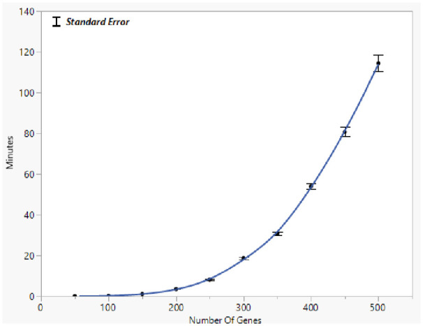
Running time of the graphical lasso with the increasing number of gene variables. The point on the curve indicates the average time. The running time was collected through 10 experiments for each size indicated in the x-axis.

Discussion

Undoubtedly, a global network including all genes provides additional information for the analysis of human diseases and will be more helpful for biologists to acquire insights into the genetic interactions than a subnetwork. Owing to the nature of Monte Carlo sampling, the sampled subdatasets are independent, and therefore, the estimated subnetworks are also independent. The MCGGM model can also be effectively deployed on a parallel computing platform to infer global networks.

The proposed MCGGM is based on GGM and speeds up the estimation of GGM in learning global genetic networks at a genome-wide scale. The challenge is that MCGGM introduces “false positive” interactions between genes during the estimation. Although the threshold was set to filter the “false positive” gene interactions, some “false positive” gene interactions could not be eliminated from the estimated networks. However, moderate FPs may be tolerated. Also, because of the intrinsic attribute of random sampling, there is a small probability that some gene interactions might not be estimated because those gene pairs might not be sampled in the same subset. But the possibility of losing highly dependent gene interactions can be reduced by setting up a statistically acceptable threshold. The estimated results show that, even if the interactions between some gene pairs are never estimated directly, if they are highly conditionally dependent, their undirected interactions can be identified via a short path with a high probability. Actually, the probability of losing highly dependent gene interactions will be far less than the statistically acceptable threshold.

Despite the existing challenges and minor limitations, the proposed method has been proven to be efficient in learning global gene networks on genome-wide data sets.

Conclusions

The proposed MCGGM model integrates traditional GGM and Monte Carlo simulation technique to make learning a global genetic network from genome-wide data set practical. The integrated model MCGGM was tested and verified using several RNA-seq gene expression data sets. The results demonstrate that MCGGM is an efficient and robust model to be deployed to learn global genetic networks from genome-wide gene expression data sets. The estimated interactions in genome-wide expression data sets provide insights for biologists to explore the complicated molecular interactions and also shed light on exploring new mechanisms of pathways which are involved in different biological activities.

References

- 1. Stolovitzky G, Monroe D, Califano A. Dialogue on reverse-engineering assessment and methods: the DREAM of high-throughput pathway inference. Ann N Y Acad Sci. 2017;1115:1-22. doi: 10.1196/annals.1407.021 [DOI] [PubMed] [Google Scholar]
- 2. Jensen FV. An Introduction to Bayesian Networks. UCL Press; 1996. [Google Scholar]
- 3. Friedman N, Linial M, Nachman I, Pe’er D. Using Bayesian networks to analyze expression data. J Comput Biol. 2000;7:601-620. doi: 10.1089/106652700750050961 [DOI] [PubMed] [Google Scholar]
- 4. Hartemink A, Gifford D, Jaakkola T, Young R. Using graphical models and genomic expression data to statistically validate models of genetic regulatory networks. Pac Symp Biocomput. 2001:422-433. doi: 10.1142/9789814447362_0042 [DOI] [PubMed] [Google Scholar]
- 5. Imoto S, Goto T, Miyano S. Estimation of genetic networks and functional structures between genes by using Bayesian networks and nonparametric regression. Pac Symp Biocomput. 2002:175-186. doi: 10.1142/9789812799623_0017 [DOI] [PubMed] [Google Scholar]
- 6. Tamada Y, Kim S, Bannai H, et al. Estimating gene networks from gene expression data by combining Bayesian network model with promoter element detection. Bioinformatics. 2003;19:ii227-ii236. doi: 10.1093/bioinformatics/btg1082 [DOI] [PubMed] [Google Scholar]
- 7. Husmeier D. Sensitivity and specificity of inferring genetic regulatory interactions from microarray experiments with dynamic Bayesian networks. Bioinformatics. 2003;19:2271-2282. doi: 10.1093/bioinformatics/btg313 [DOI] [PubMed] [Google Scholar]
- 8. Yu J, Smith VA, Wang PP, Hartemink AJ, Jarvis ED. Advances to Bayesian network inference for generating causal networks from observational biological data. Bioinformatics. 2004;20:3594-3603. doi: 10.1093/bioinformatics/bth448 [DOI] [PubMed] [Google Scholar]
- 9. Kim S, Imoto S, Miyano S. Dynamic Bayesian network and nonparametric regression for nonlinear modeling of gene networks from time series gene expression data. Biosystems. 2004;75:57-65. doi: 10.1016/j.biosystems.2004.03.004 [DOI] [PubMed] [Google Scholar]
- 10. Zou M, Conzen SD. A new dynamic Bayesian network (DBN) approach for identifying gene regulatory networks from time course microarray data. Bioinformatics. 2005;21:71-79. doi: 10.1093/bioinformatics/bth463 [DOI] [PubMed] [Google Scholar]
- 11. Chickering DM. Learning Bayesian networks is NP-complete. In: Fisher D, Lenz HJ, eds. Learning from Data. Springer; 1996:121-130. [Google Scholar]
- 12. Cohen J, Cohen P, West SG, Aiken LS. Applied Multiple Regression/Correlation Analysis for the Behavioral Sciences. 2nd ed. Psychology Press; 2002. [Google Scholar]
- 13. Langfelder P, Horvath S. WGCNA: an R package for weighted correlation network analysis. BMC Bioinformatics. 2008;9:559. https://bmcbioinformatics.biomedcentral.com/articles/10.1186/1471-2105-9-559 [DOI] [PMC free article] [PubMed] [Google Scholar]
- 14. Jansen R, Greenbaum D, Gerstein M. Relating whole-genome expression data with protein-protein interactions. Genome Res. 2002;12:37-46. http://www.genome.org/cgi/doi/10.1101/gr.205602 [DOI] [PMC free article] [PubMed] [Google Scholar]
- 15. Emilsson V, Thorleifsson G, Zhang B, et al. Genetics of gene expression and its effect on disease. Nature. 2008;452:423-428. 10.1038/nature06758 [DOI] [PubMed] [Google Scholar]
- 16. Li J, LJ. Adjusting multiple testing in multilocus analyses using the eigenvalues of a correlation matrix. Heredity (Edinb). 2005;95:221-227. 10.1038/sj.hdy.6800717 [DOI] [PubMed] [Google Scholar]
- 17. Lieberman-Aiden E, van Berkum NL, et al. Comprehensive mapping of long-range interactions reveals folding principles of the human genome. Science. 2009;326:289-293. 10.1126/science.1181369 [DOI] [PMC free article] [PubMed] [Google Scholar]
- 18. Shabalin A. Matrix eQTL: ultra fast eQTL analysis via large matrix operations. Bioinformatics. 2012;28:1353-1358. 10.1093/bioinformatics/bts163 [DOI] [PMC free article] [PubMed] [Google Scholar]
- 19. Ge H, Liu Z, Church GM, Vidal M. Correlation between transcriptome and interactome mapping data from Saccharomyces cerevisiae. Nat Genet. 2001;29:482-486. 10.1038/ng776 [DOI] [PubMed] [Google Scholar]
- 20. Edwards D. Introduction to Graphical Modelling. Springer-Verlag; 2000. [Google Scholar]
- 21. Whittaker J. Graphical Models in Applied Multivariate Statistics. Wiley Publishing; 2009. [Google Scholar]
- 22. Drton M, Perlman MD. Model selection for Gaussian concentration graphs. Biometrika. 2004;91:591-602. doi: 10.1093/biomet/91.3.59 [DOI] [Google Scholar]
- 23. Tibshirani R. Regression shrinkage and selection via the lasso. J R Stat Soc Ser B Methodol. 1996; 58:267-288. doi: 10.1111/j.2517-6161.1996.tb02080.x [DOI] [Google Scholar]
- 24. Li H, Gui J. Gradient directed regularization for sparse Gaussian concentration graphs, with applications to inference of genetic networks. Biostatistics. 2005;7:302-317. doi: 10.1093/biostatistics/kxj008 [DOI] [PubMed] [Google Scholar]
- 25. Meinshausen N, Buhlmann P. High-dimensional graphs and variable selection with the Lasso. Ann Stat. 2006;34:1436-1462. doi: 10.1214/009053606000000281 [DOI] [Google Scholar]
- 26. Yuan M, Lin Y. Model selection and estimation in the Gaussian graphical model. Biometrika. 2007;94:19-35. doi: 10.1093/biomet/asm018 [DOI] [Google Scholar]
- 27. Friedman J, Hastie T, Tibshirani R. Sparse inverse covariance estimation with the graphical lasso. Biostatistics. 2008;9:432-441. doi: 10.1093/biostatistics/kxm045 [DOI] [PMC free article] [PubMed] [Google Scholar]
- 28. Liu H, Roeder K, Wasserman L. Stability approach to regularization selection (StARS) for high dimensional graphical models. Paper presented at: NIPS’10 Proceedings of the 23rd International Conference on Neural Information Processing Systems; December 6-9, 2010; Vancouver, BC, Canada;2:1432-1440. https://dl.acm.org/doi/abs/10.5555/2997046.2997056 [PMC free article] [PubMed] [Google Scholar]
- 29. Dobra A, Lenkoski A, et al. Bayesian inference for general Gaussian graphical models with application to multivariate lattice data. J Am Stat Assoc. 2010;106:1418-1433. doi: 10.1198/jasa.2011.tm10465 [DOI] [PMC free article] [PubMed] [Google Scholar]
- 30. Wang H. Bayesian graphical lasso models and efficient posterior computation. Bayesian Anal. 2012;7:867-886. doi: 10.1214/12-BA729 [DOI] [Google Scholar]
- 31. Danaher P, Wang P, Witten DM. The joint graphical lasso for inverse covariance estimation across multiple classes. J R Stat Soc Ser B Stat Methodol. 2014;76:373-397. doi: 10.1111/rssb.12033 [DOI] [PMC free article] [PubMed] [Google Scholar]
- 32. Zhang L, Kim S. Learning gene networks under SNP perturbations using eQTL datasets. PLoS Comput Biol. 2014;10:e1003420. doi: 10.1371/journal.pcbi.1003420 [DOI] [PMC free article] [PubMed] [Google Scholar]
- 33. Ren Z, Sun T, Zhang C, Zhou HH. Asymptotic normality and optimalities in estimation of large Gaussian graphical models. Ann Statist.2015;43: 991-1026. doi: 10.1214/14-AOS1286 [DOI] [Google Scholar]
- 34. Janková J, van de Geer S. Confidence intervals for high-dimensional inverse covariance estimation. Electron J Statist. 2015;9:1205-1229. doi: 10.1214/15-EJS1031 [DOI] [Google Scholar]
- 35. Gu Q, Cao Y, Ning Y, Liu H. Local and global inference for high dimensional Gaussian copula graphical models. Arxiv [preprint]. 2015. Arxiv.org/abs/1502.02347. [Google Scholar]
- 36. Ning Y, Liu H. A general theory of hypothesis tests and confidence regions for sparse high dimensional models. Arxiv [preprint]. 2014. Arxiv.org/abs/1412.8765. [Google Scholar]
- 37. Kumari S, Deng W, Gunasekara C, et al. Bottom-up GGM algorithm for constructing multilayered hierarchical gene regulatory networks that govern biological pathways or processes. BMC Bioinformatics. 2016;17:132. doi: 10.1186/s12859-016-0981-1 [DOI] [PMC free article] [PubMed] [Google Scholar]
- 38. Banerjee O, Ghaoui LE, d’Aspremont A. Model selection through sparse maximum likelihood estimation for multivariate Gaussian or binary data. J Mach Learn Res. 2008;9:485-516. [Google Scholar]
- 39. Leclerc RD. Survival of the sparsest: robust gene networks are parsimonious. Mol Syst Biol. 2008;4:213. doi: 10.1038/msb.2008.52 [DOI] [PMC free article] [PubMed] [Google Scholar]
- 40. Hammersley JM, Handscomb DC. Monte Carlo Methods. Halsted Press; 1964. [Google Scholar]
- 41. Eckhardt R. Stan Ulam, John von Neumann, and the Monte Carlo method. Los Alamos Sci. 1987; Special Issue: 131-137. [Google Scholar]
- 42. Hastings WK. Monte Carlo sampling methods using Markov chains and their applications. Biometrika. 1970;57:97-109. doi: 10.2307/2334940 [DOI] [Google Scholar]
- 43. Ojeda P, Garcia ME, Londoño A, Chen NY. Monte Carlo simulations of proteins in cages: influence of confinement on the stability of intermediate states. Biophys J. 2009;96:1076-1082. doi: 10.1529/biophysj.107.125369 [DOI] [PMC free article] [PubMed] [Google Scholar]
- 44. Cassey AJ, Smith BO. Simulating confidence for the Ellison-Glaeser index. J Urban Econ. 2014;81:93. doi: 10.1016/j.jue.2014.02.005 [DOI] [Google Scholar]
- 45. Ciancarini P, Favini GP. Monte Carlo tree search in Kriegspiel. Artif Intell. 2010;174:670-684. doi: 10.1016/j.artint.2010.04.017 [DOI] [Google Scholar]
- 46. Kroese DP, Brereton T, Taimre T, Botev ZI. Why the Monte Carlo method is so important today. WIREs Comput Stat. 2014;6:386-392. doi: 10.1002/wics.1314 [DOI] [Google Scholar]
- 47. KEGG: Kyoto encyclopedia of genes genomes. Accessed February 1, 2018. https://www.genome.jp/kegg/
- 48. GDCDP: genomic data commons data portal. Accessed February 1, 2018. https://portal.gdc.cancer.gov/
- 49. Fawcett T. An introduction to ROC analysis. Pattern Recognit Lett. 2006;27:861-874. doi: 10.1016/j.patrec.2005.10.010 [DOI] [Google Scholar]
- 50. Niwattanakul S, Singthongchai J, et al. Using of Jaccard coefficient for keywords similarity. Paper presented at: Proceedings of the International Multiconference of Engineers and Computer Scientists; March 13-15, 2013; Hong Kong. https://www.iaeng.org/publication/IMECS2013/IMECS2013_pp380-384.pdf [Google Scholar]
- 51. Kishore U, Reid KB. C1q: structure, function, and receptors. Immunopharmacology. 2010;49:159-170. doi: 10.1016/S0162-3109(00)80301-X [DOI] [PubMed] [Google Scholar]
- 52. Ghebrehiwet B, Hosszu KK, et al. The C1q family of proteins: insights into the emerging non-traditional functions. Front Immunol. 2012;3:52. doi: 10.3389/fimmu.2012.00052 [DOI] [PMC free article] [PubMed] [Google Scholar]
- 53. Walport MJ. Complement. N Engl J Med. 2001;344:1058-1066. doi: 10.1056/nejm200104123441506 [DOI] [PubMed] [Google Scholar]
- 54. Kapp LD, Lorsch JR. The molecular mechanics of eukaryotic translation. Annu Rev Biochem. 2004;73:657-704. doi: 10.1146/annurev.biochem.73.030403.080419 [DOI] [PubMed] [Google Scholar]
- 55. Kapp LD, Lorsch JR. Gtp-dependent recognition of the methionine moiety on initiator tRNA by translation factor eIF2. J Mol Biol. 2004;335:923-936. doi: 10.1016/j.jmb.2003.11.025 [DOI] [PubMed] [Google Scholar]
- 56. Dong Z, Zhang J. Initiation factor eIF3 and regulation of mRNA translation, cell growth, and cancer. Crit Rev Oncol Hematol. 2006;59:169-180. doi: 10.1016/j.critrevonc.2006.03.005 [DOI] [PubMed] [Google Scholar]
- 57. Bhat M, Robichaud N, Hulea L, Sonenberg N, Pelletier J, Topisirovic I. Targeting the translation machinery in cancer. Nat Rev Drug Discov. 2015;14:261-278. doi: 10.1038/nrd4505 [DOI] [PubMed] [Google Scholar]
- 58. Hershey JW. The role of eIF3 and its individual subunits in cancer. Biochim Biophys Acta. 2015;1849:792-800. doi: 10.1016/j.bbagrm.2014.10.005 [DOI] [PubMed] [Google Scholar]
- 59. Zhang F, Xiang S, Cao Y, et al. EIF3D promotes gallbladder cancer development by stabilizing GRK2 kinase and activating PI3K-AKT signaling pathway. Cell Death Dis. 2017;8:e2868. doi:10.1038%2Fcddis.2017.263 [DOI] [PMC free article] [PubMed] [Google Scholar]
- 60. Wang D, Jia Y, Zheng W, Li C, Cui W. Overexpression of eIF3D in lung adenocarcinoma is a new independent prognostic marker of poor survival. Dis Markers. 2019;2019:6019637. doi: 10.1155/2019/6019637 [DOI] [PMC free article] [PubMed] [Google Scholar]
- 61. Chai R, Wang N, Chang Y, et al. Systematically profiling the expression of eIF3 subunits in glioma reveals the expression of eIF3i has prognostic value in IDH-mutant lower grade glioma. Cancer Cell Int. 2019;19:155. doi: 10.1186/s12935-019-0867-1 [DOI] [PMC free article] [PubMed] [Google Scholar]
- 62. Thornton S, Anand N, Purcell D, Lee J. Not just for housekeeping: protein initiation and elongation factors in cell growth and tumorigenesis. J Mol Med (Berl). 2003;81:536-548. doi: 10.1007/s00109-003-0461-8 [DOI] [PubMed] [Google Scholar]
- 63. Tatsuka M, Mitsui H, Wada M, Nagata A, Nojima H, Okayama H. Elongation factor-1α gene determines susceptibility to transformation. Nature. 1992;359:333-336. doi: 10.1038/359333a0 [DOI] [PubMed] [Google Scholar]
- 64. Lamberti A, Caraglia M, et al. The translation elongation factor 1A in tumorigenesis, signal transduction and apoptosis: review article. Amino Acids. 2004;26:443-448. doi: 10.1007/s00726-004-0088-2 [DOI] [PubMed] [Google Scholar]
- 65. Chuang S, Chen L, Lambertson D, Anand M, Kinzy TG, Madura K. Proteasome-mediated degradation of cotranslationally damaged proteins involves translation elongation factor 1A. Mol Cell Biol. 2005;25:403-413. doi: 10.1128/MCB.25.1.403-413.2005 [DOI] [PMC free article] [PubMed] [Google Scholar]
- 66. Grant AG, Flomen RM, Tizard ML, Grant DA. Differential screening of a human pancreatic adenocarcinoma λgt11 expression library has identified increased transcription of elongation factor EF-1 alpha in tumour cells. Int J Cancer. 1992;50:740-745. doi: 10.1002/ijc.2910500513 [DOI] [PubMed] [Google Scholar]
- 67. Zhang L, Zhou W, Velculescu VE, et al. Gene expression profiles in normal and cancer cells. Science. 1997;276:1268-1272. doi: 10.1126/science.276.5316.1268 [DOI] [PubMed] [Google Scholar]
- 68. Johnsson A, Zeelenberg I, Min Y, et al. Identification of genes differentially expressed in association with acquired cisplatin resistance. Br J Cancer. 2000;83:1047-1054. doi: 10.1054/bjoc.2000.1420 [DOI] [PMC free article] [PubMed] [Google Scholar]
- 69. Xie D, Jauch A, Miller CW, Bartram CR, Koeffler HP. Discovery of over-expressed genes and genetic alterations in breast cancer cells using a combination of suppression subtractive hybridization, multiplex FISH and comparative genomic hybridization. Int J Oncol. 2002;21:499-507. doi: 10.3892/ijo.21.3.499 [DOI] [PubMed] [Google Scholar]
- 70. Mohler JL, Morris TL, Ford OH, 3rd, Alvey RF, Sakamoto C, Gregory CW. Identification of differentially expressed genes associated with androgen-independent growth of prostate cancer. Prostate. 2002;51:247-255. doi: 10.1002/pros.10086 [DOI] [PubMed] [Google Scholar]
- 71. de Wit NJ, Burtscher HJ, Weidle UH, Ruiter DJ, van Muijen GN. Differentially expressed genes identified in human melanoma cell lines with different metastatic behavior using high density oligonucleotide arrays. Melanoma Res. 2002;12:57-69. doi: 10.1097/00008390-200202000-00009 [DOI] [PubMed] [Google Scholar]
- 72. Blanch A, Robinson F, Watson IR, Cheng LS, Irwin MS. Eukaryotic translation elongation factor 1-alpha 1 inhibits p53 and p73 dependent apoptosis and chemotherapy sensitivity. PLoS ONE. 2013;8:e66436. doi: 10.1371/journal.pone.0066436 [DOI] [PMC free article] [PubMed] [Google Scholar]