

SUMMARY
Color-biased regions have been found between face- and place-selective areas in the ventral visual pathway. To investigate the function of the color-biased regions in a pathway responsible for object recognition, we analyzed the Natural Scenes Dataset (NSD), a large 7T fMRI dataset from 8 participants who viewed up to 30,000 trials of images of colored natural scenes over more than 30 scanning sessions. In a whole-brain analysis, we correlated the average color saturation of the images with voxel responses, revealing color-biased regions that diverge into two streams, beginning in V4 and extending medially and laterally relative to the fusiform face area in both hemispheres. We drew regions of interest (ROIs) for the two streams and found that the images for each ROI that evoked the largest responses had certain characteristics: they contained food, circular objects, warmer hues, and had higher color saturation. Further analyses showed that food images were the strongest predictor of activity in these regions, implying the existence of medial and lateral ventral food streams (VFSs). We found that color also contributed independently to voxel responses, suggesting that the medial and lateral VFSs use both color and form to represent food. Our findings illustrate how high-resolution datasets such as the NSD can be used to disentangle the multifaceted contributions of many visual features to the neural representations of natural scenes.
Keywords: food, color vision, fMRI, ventral food stream, VFS, ventral visual pathway, natural scenes
In Brief
What is the role of color-biased regions in the ventral visual pathway? Pennock et al. redefine our understanding of color-biased regions by showing that they respond to both food and color. Their findings suggest that color contributes to the visual representa representation of food.
INTRODUCTION
The ventral visual pathway is specialized for the perception and recognition of visual objects, e.g. faces1,2, places3,4, bodies5,6, and words7,8. Color is an important feature of objects9,10, and color biased regions have been found in the ventral visual pathway anterior to V411–19. But are there supraordinate object specialisms associated with the color biases observed in these regions?
The processing of color information begins in the retina with a comparison of the activities of the three classes of cone that are sensitive to short (S), medium (M) and long (L) wavelengths of light. Subsequently, different classes of retinal ganglion cells send luminance and color information to the lateral geniculate nucleus which projects to V120. In the early visual cortices such as V1, V2, V3 and V4v, responsiveness to hue and saturation as color attributes has been studied using functional magnetic resonance imaging (fMRI)16,21–28. V1 to V3 respond to color among other features29,30, while V4 and the ventral occipital region (VO; anterior to V4) are thought to be specialized for processing color31. Voxel activity patterns in V4, VO1 and VO2 can strongly distinguish chromatic from achromatic stimuli32, and clustering and representational similarity analyses have provided evidence for a representation of color in these areas32–34. More cognitive color tasks are also associated with V4, such as mental imagery for color23 and color memory24. As color information progresses through visual cortical regions, its representation likely becomes transformed to aid cognitive tasks such as object perception12,14,35,36, and color representations in these regions are known to be modulated by other object features such as shape and animacy36. In particular, Rosenthal et al.36 found that the color tuning properties of neurons in macaque IT correlated with the warm colors typical of salient objects37.
Most studies of color perception present simple stimuli such as color patches, rather than color as it occurs in natural scenes. However, in daily life our visual system encounters colors as part of conjunctions of object features integrated in context within natural scenes. With simple stimuli, color is dissociated from its regular context and meaning: Such stimuli have basic spatial form, may be selected from a restricted color gamut, and are typically presented on a uniform surround. Visual responses to carefully controlled colored stimuli might be quite different from responses to colors in their complex, naturalistic settings. For example, for colored patches, decoding accuracy drops progressively from V1 to V422,23, while for colored object categories decoding accuracy increases through the same areas35. To understand how the brain represents color in its usual contexts, and to understand the functions of the color biased regions in the ventral visual pathway, it is therefore crucial to use complex stimuli containing a variety of object categories such as natural scenes11–13.
We aimed to characterize the neural representation of color and its association with the representation of objects and other image properties as they are encountered in natural scenes. The Natural Scenes Dataset (NSD)38 provides a unique opportunity for this endeavor. It is an unprecedented large-scale fMRI dataset in which each participant viewed thousands of colored (and some greyscale) natural scenes over 30 to 40 sessions in a 7T scanner. This dataset therefore has impressively high signal-to-noise and statistical power39. However, images of natural scenes are high-dimensional and visual features can correlate with one another strongly, making it challenging to accurately disentangle contributions of different features. Nonetheless, with its huge number of well-characterized and segmented stimulus images, the NSD is one of the best datasets currently available to uncover the neural representations underlying perception of natural scenes38,40.
Our analyses revealed two streams in the ventral visual pathway that exhibit responses to color in the NSD images. We found that both streams were primarily responsive to food objects, implying that color is a key part of the neural representation of food in these ventral visual areas. Our findings are bolstered by two recent papers also finding strong evidence for food selectivity in these regions of the ventral visual pathway using distinct data-driven approaches with the NSD41,42, and an additional fMRI study presenting isolated food images42.
RESULTS
Identifying color-biased regions in the ventral visual pathway
To isolate responses to chromatic compared to achromatic information in the NSD images we conducted a whole-brain correlation between the average color saturation of each NSD image and the BOLD signal change observed at each voxel (Figure 1A). Since saturation and luminance (Figures 2A and S1A) are correlated in natural scenes43, we used the mean luminance of each image as a covariate. The correlations were Bonferroni corrected for each participant based on the number of voxels in participant-native space. We also conducted an analysis to measure split-half reliability, where voxel-by-voxel correlation coefficients for average saturation and voxel responses were correlated over the whole brain for odd and even images.
Figure 1: Correlations between average saturation and voxel responses.
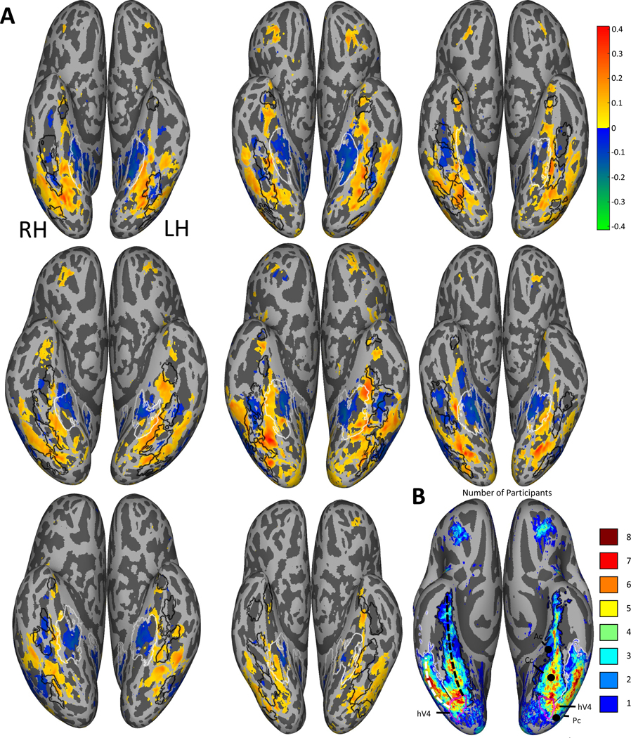
(A) Pearson correlation maps of the ventral view in native participant space on an inflated cortical surface (top-left is participant 1, bottom-middle is participant 8; going left to right). The maps show for each voxel the correlation between the mean saturation of each image and the corresponding voxel responses, with mean luminance as a covariate. Positive correlations are displayed in red and yellow, and negative correlations in green and blue. Only correlations with significant whole brain Bonferroni-corrected p-values are plotted, showing two color-responsive regions in the ventral visual pathway starting in V4 and diverging medially and laterally of the fusiform face area. Black contours indicate face-selective brain regions for each individual participant (FFA-1, FFA-2, OFA, mTL-faces and ATL-faces) and white contours indicate place-selective areas for each individual participant (PPA and RSC); for a description of how these regions were defined see Allen et al.38.
(B) The number of participants showing overlapping significant positive voxels in fsaverage space. On the right hemisphere, the medial stream is indicated by the black dashed line and the lateral stream by the white dashed line. On the left hemisphere the coordinates of the color-biased regions identified by Lafer-Sousa et al.11 are shown (Ac, Cc, Pc). For both hemispheres, hV4 from the brain atlas by Wang et al.71 is indicated by the magenta contours, the medial ROIs are indicated with black contours and the lateral ROIs with white contours.
Figure 2: Montages of images evoking the lowest and highest ROI responses and showing variation in each image statistic.
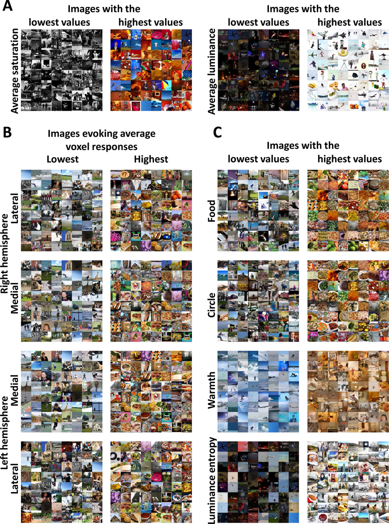
(A) Montages of the 68 images with the highest (right montages) and lowest (left montages) values for the image statistics included in the correlation analysis: average saturation and average luminance for Participant 1. See Figure S1A for montages for the other participants.
(B) Montages of the 68 images for the lateral and medial ROIs for both hemispheres that evoked the highest (right montages) and lowest (left montages) averaged z-scored voxel responses for Participant 1. See Figure S1B for montages for the other participants.
(C) Montages of the 68 images with the lowest and highest values for four further image statistics are shown for Participant 1: number of food pixels (food), number of pixels forming circular objects (circle), average warmth rating of pixel colors (warmth) and luminance entropy. The right column contains montages of images with the highest values for each image statistic and the left column contains montages of images with the lowest values for each image statistic. See Figure S1A for montages for the other participants.
For all participants we found areas showing positive correlations between saturation and voxel responses in the ventral visual pathway (Figure 1), with strong correlations in V4 and diverging into two distinct streams which we divided into medial and lateral regions of interest (ROIs). The medial ROI is located between face and place areas (fLoc-defined areas are shown in Figure 1A and the ROI boundaries in Figure 1B; see fLoc-experiment by Allen et al.38), and is roughly in agreement with the location of the color-biased regions identified by Lafer-Sousa et al.11 (Figure 1B). We conducted a whole brain split-half reliability analysis on the correlation between voxel responses and saturation, which showed high reliability, with r = 0.82 (range = 0.71 – 0.89 for different participants).
For all 8 participants there were also areas that showed negative correlations between saturation and voxel responses, specifically the PPA and the region located between the lateral and medial ROIs that showed positive correlations (Figure 1A). For seven participants there was an area of negative correlation lateral of the lateral ROI, roughly corresponding to area MT. For six participants (and one further participant in the left hemisphere only) there was a positive correlation with saturation in prefrontal regions (Figure 1A), reminiscent of other findings on color processing in the prefrontal cortex44–46. Several participants also showed significant correlations between saturation and voxel responses in earlier visual areas V1-V3.
Montages of images producing the highest and lowest voxel responses
Our correlation analysis between BOLD and saturation revealed areas responsive to color in the ventral visual pathway for all participants. To better understand stimulus representation in these areas, we created montages of the images that evoked the highest and lowest voxel responses for these areas, split into four ROIs (medial and lateral, left and right hemispheres; Figure 2B for participant 1 and Figure S1B for the other participants).
By inspecting the montages, we identified multiple image properties present in images evoking the highest responses but not in images evoking the lowest responses. These properties were food such as bananas, donuts, and pizzas; circular objects such as plates, clocks and stop signs; warm colors such as reds and oranges; and luminance entropy (how well or poorly luminance values in one location can predict the values in nearby locations47,48). These image characteristics were consistent across all participants, the medial and lateral ROIs, and both hemispheres, suggesting that the four ROIs all process a similar type of visual information.
No large differences in images statistics between participants
In order to allow a quantitative analysis of voxel responses to the image properties that appeared to distinguish images that evoked the higher and lower voxel responses in our ROIs we calculated an image statistic for each image property. We also included mean luminance as an image statistic as it was used as a covariate in the correlation analysis with saturation. Our image statistics were mean saturation, pixel count for food objects, pixel count for circular objects, mean warmth ratings over the colors of all pixels, luminance entropy and mean luminance (see STAR Methods for a detailed description). For food and circular objects we used pixel count contained within the segmented objects to create continuous variables that could be entered into further analyses along with the other continuous variables. Our assumption was that there is a monotonic relationship between the pixel sizes of these objects and voxel responses, though we did not assume that the relationship has any particular form. There is some evidence to suggest that this is a reasonable assumption49, though voxel responses may also depend on other properties of object images, such as real-world size or orientation, which are not captured by the metric.
The six image statistics were significantly intercorrelated (see Figure S2B for correlation matrices of image statistics for each participant and Figure 2A and 2C for montages). Average luminance and luminance entropy were strongly positively correlated (group average ρ = 0.68), and circular object pixel count and food pixel count were moderately correlated (group average ρ = 0.42). Besides one exception, all other pairs of image statistics had low but significant correlations (group average ρ < 0.30). Circular object pixel count and luminance entropy were not significantly correlated for seven of the eight participants. The relationships between image statistics were highly consistent between participants, even though different participants viewed largely non-overlapping image sets (0.9993 ≤ ρ ≤ 0.9999 for pairwise correlations between image statistic correlation matrices between participants). This suggests there were no substantial differences in image statistics between participants.
Relationship between image statistics and average ROI responses
We investigated the relationship between each image statistic and average voxel responses for the four ROIs (medial and lateral areas in both hemispheres) that we had defined based on correlations between voxel responses and average saturation. We plotted moving average ROI responses against each of the image statistics (Figure 3A). ROI responses show positive linear relationships with average saturation and mean warmth ratings of pixel colors. ROI responses show positive non-linear (decelerating) relationships with food pixel count and circular object pixel count, with a higher gain for food pixel count than for any of the other image statistics. There was no relationship between ROI responses and luminance entropy, and a small negative relationship between ROI responses and average luminance. The findings were consistent across hemispheres and ROIs for all eight participants (see Figure S2A for results for individual participants).
Figure 3: ROI responses to image statistics.

(A) Mean z-scored voxel responses in the medial and lateral ROIs of the left and right hemispheres. Each x-axis shows an image statistic: mean image saturation, number of pixels that are contained in food objects, number of pixels that are contained in circular objects, mean warmth ratings of pixel colors, luminance (L+M) entropy48, and mean luminance. The y-axes show the mean z-scored voxel responses. In each case the images were sorted from lowest to highest based on the image statistic. Then a running average of mean z-scored voxel responses for sets of 500 images was plotted (1–500, 2–501, 3–502, etc.), averaged across all participants. Error bars are within-participant 95% confidence intervals. Plots for individual participants are shown in Figure S2A.
(B) Effects of food and saturation on mean z-scored voxel responses for all four ROIs (left (LH) and right (RH) hemispheres, and medial and lateral ROIs). The orange lines show mean z-scored voxel responses for images that contained food and the green lines for images that did not contain food based on the COCO object categories. Error bars are within-participant 95% confidence intervals. The montages to the right show randomly selected images from each of the four groups. Plots for individual participants are shown in Figure S5 and ANOVA results for individual participants are shown in Table S2. For the results of equivalent analyses for object pixels only, see Figures S4A and S5, and Table S4.
(C) Effects of food and mean rating of warmth for colors of all pixels on mean z-scored voxel responses. The orange lines show mean z-scored voxel responses for images that contained food and the green lines for images that did not contain food based on the COCO object categories. Error bars are within-participant 95% confidence intervals. The montages to the right show randomly selected images from each of the four groups. Plots for individual participants are shown in Figure S5 and ANOVA results for individual participants are shown in Table S3. For the results of equivalent analyses for object pixels only, see Figures S4B and S5, and Table S5.
Food is the strongest predictor for responses in the color-biased ROIs
We included the six image statistics in a multiple linear regression to identify the best predictors for the average z-scored voxel responses for our four ROIs (see STAR Methods for details). A regression analysis showed significant relationships in all four ROIs (Medial ROI LH: mean F (6,9648) over 8 participants = 288, SD = 101.4, p < 2.04 × 10−188, mean R2 = 0.15, SD = 0.04; Medial ROI RH: mean F (6,9648) = 242.8, SD = 100.6, p < 7.02 × 10−171, mean R2 = 0.13, SD = 0.04; Lateral ROI LH: mean F (6,9648) = 218, SD = 95.4, p < 1.19 × 10−114, mean R2 = 0.12, SD = 0.04; Lateral ROI RH: mean F (6,9648) = 210, SD =97.4, p < 4.98 × 10−120, mean R2 = 0.11, SD = 0.04). Summary results in Table 1 showed that food is the strongest predictor for all four ROIs in all eight participants. Individual results for each participant are available in Table S1.
Table 1.
Multiple linear regression beta coefficients for the four ROIs.
| Multiple linear regression beta coefficients | |||||||
|---|---|---|---|---|---|---|---|
|
| |||||||
| B0 | Average Saturation | Food | Circles | Warmth | Luminance Entropy | Average Luminance | |
|
| |||||||
| Medial Left | 5.3863 × 10⁻⁹ | 0.0563 | 0.1950 | 0.0608 | 0.0320 | 0.0446 | − 0.0516 |
| Medial Right | 5.4712 × 10⁻⁹ | 0.0553 | 0.1598 | 0.0596 | 0.0294 | 0.0439 | − 0.0473 |
| Lateral Left | 9.9330 × 10⁻¹² | 0.0343 | 0.2336 | 0.0402 | 0.0279 | − 0.0047 | − 0.0029 |
| Lateral Right | 1.7063 × 10⁻⁹ | 0.0391 | 0.2367 | 0.0272 | 0.0442 | − 0.0089 | 0.0010 |
Average beta coefficients for each image statistic in the multiple linear regressions to predict average voxel responses, for each of the four ROIs. See Table S1 for results of multiple linear regressions for individual participants.
There are no sub-clusters of voxels that prefer color over food within the ROIs
To test whether there are sub-clusters of voxels within these ROIs that respond to different image statistics we also ran multiple linear regressions on all the individual voxels that showed a significant positive (Bonferroni-corrected) correlation with saturation for each participant. For each voxel we identified the image statistic with the largest beta coefficient (Figure 4). Food pixel count produced the first ranked beta coefficient in the single-voxel multiple regressions for almost all voxels, suggesting that food is the strongest predictor for all four ROIs even at an individual voxel level. For the left medial, left lateral, right medial and right lateral ROIs respectively, 78%, 92%, 69% and 92% of voxels included in the multiple regressions had food as the strongest predictor, and only 4%, 0.6%, 7% and 2% had saturation as the strongest predictor. For the other image statistics there was no consistent pattern. Voxel activity in early visual areas was most strongly predicted by luminance entropy. For V1 voxels defined by the HCPMMP 1.0 atlas50, 80% of voxels included in the multiple regressions had luminance entropy for the first ranked beta coefficient, 7% had food and 2% had saturation. The results of our single-voxel multiple linear regressions suggest that food is the main predictor for most voxels in the ROIs and there are no substantial sub-clusters of voxels responding most strongly to other image statistics.
Figure 4. Strongest predictors in single voxel multiple linear regressions for voxels responsive to color saturation.

For each of the eight participants flattened whole-brain cortical maps are shown in fsaverage space. Each voxel that showed a significant positive (Bonferroni-corrected) correlation with average saturation was included in the single-voxel multiple regressions, and is colored in the figure according to the image statistic that had the largest beta coefficient in the multiple regression for that voxel. Within the ROIs there are no substantial sub-clusters of voxels for which the strongest predictors in the single-voxel multiple linear regressions are not food.
Color contributes independently to ROI responses in the absence of food
The multiple linear regressions for the ROIs showed that food pixel count had the highest beta coefficients of the six image statistics. The results of our whole-brain correlation with saturation and previous literature11 imply that these areas are responsive to color. We therefore sought to further investigate the contributions of saturation, color warmth and food to ROI responses by conducting two-way ANOVAs (Figure 3B), one with factors for food and mean saturation and one with factors for food and mean warmth rating of pixel colors. For these ANOVAs we defined 4 groups of images, one with food and with high saturation or warmth (depending on the ANOVA), one without food and with high saturation or warmth, one with food and with low saturation or warmth and one without food and with low saturation or warmth. Importantly, the shapes of histograms of the image statistics for the food and non-food groups of images were exactly matched (see STAR Methods and Figure S3). Mean z-scored voxel responses for each ROI averaged across the 8 participants are shown for food and saturation in Figure 3B and for food and warmth in Figure 3C. Both figures show a large difference between voxel responses for food versus non-food images in the ROIs, and smaller differences between voxel responses for high versus low saturation and high versus low warmth. The ANOVA with factors for food and saturation revealed a significant main effect for food for all eight participants and all four ROIs (mean F = 309, p < 6 × 10⁻²⁶). All four ROIs also showed a significant main effect of saturation for all eight participants (mean F = 59, 2 × 10⁻³⁰ < p < 2 × 10⁻⁷). There were significant interactions for some participants in some ROIs. For ANOVA results for all participants, see Figure S5 and Table S2. The ANOVA with factors for food and warmth also revealed a significant main effect of food for all eight participants for all four ROIs (mean F = 371, p < 3 × 10⁻³²), and a significant main effect of warmth for all participants and ROIs, other than for Participant 6 for the medial area in the LH (mean F = 28, 2 × 10⁻¹⁸ < p < 0.1). There were significant interactions for some participants in some ROIs. For ANOVA results for all participants, see Figure S5 and Table S3.
A leading existing theory about the function of the color biased regions in the ventral visual pathway is that they represent behaviorally relevant objects, and are biased towards object-associated colors as a feature of such objects14,36. We therefore conducted further 2-way ANOVAS considering only the colors of pixels within segmented objects rather than pixels over whole images. 2-way ANOVAs with food and mean object pixel saturation as factors revealed strong significant main effects of food for all eight participants and the four ROIs, and smaller significant main effects of saturation for all eight participants and the four ROIs. The interactions were significant only for some participants in some ROIs (For group summary ANOVA results see Figure S4A, for results for individual participants see Figure S5 and Table S4). 2-way ANOVAs with food and mean object pixel warmth as factors revealed strong significant main effects of food for all eight participants and the four ROIs, and smaller significant main effects of warmth for most participants in most ROIs. The interactions were significant only for some participants in some ROIs (For group summary ANOVA results see Figure S4B, for results for individual participants see Figure S5 and Table S5). Thus, when considering object pixels only it is still clear that food is the strongest associate of responses in the ROIs. Object saturation and warmth are more weakly associated with ROI responses, independently of food.
Since the number of pixels contained in circular objects was also a relatively strong predictor of activity in the ROIs (Figure 3A) we conducted a 2-way ANOVA with factors for food and the presence or absence of segmented circular objects (circle). There was a significant main effect for food for all eight participants and all four ROIs (mean F = 741, p < 1 × 10−45), and a significant main effect of circle for only some participants in some ROIs. There were significant interactions for all participants in all ROIs except for Participant 8 in the RH medial and LH medial areas. For group results see Figure S4C and for results for individual participants see Figure S5 and Table S6.
Analysis of responses to food identifies similar regions to the color-biased areas
Our results indicate that food images are a strong predictor of responses in the ROIs, but since the ROIs were defined by responses to saturation rather than to food, the results reported so far could miss voxels that respond to food but not to saturation. We therefore conducted t-tests for each voxel on the differences between responses to images that contain food and responses to images that do not contain food. Each participant (1 to 8) saw 1284, 1284, 1176, 1237, 1303, 1240, 1309, and 1127 images of food, respectively. All other images were considered non-food images based on the Microsoft Common Objects in Context40 (COCO) object categories. Figure 5 shows results plotted for the whole brain, also including coordinates of peak activation from a fMRI meta-analysis of food images51 in the right hemisphere. We converted the Bonferroni-corrected threshold for the saturation correlation analysis (Figure 1) to a t-statistic and applied the same threshold to Figure 5 to make a comparison possible.
Figure 5. Analysis of responses to food versus non-food images.

A flattened cortical map in fsaverage space is plotted showing t-statistics (average t-values across the eight participants) for the differences between mean voxel responses for food images and mean voxel responses to non-food images. The Human Connectome Project Atlas (HCP_MMP150) is overlaid for the left hemisphere (black contours), with regions labelled where they contained voxels with significant t-statistics. On the right hemisphere are plotted white discs indicating coordinates identified by van der Laan et al.51 in a meta-analysis of brain areas responsive to food (see their Table 2), and contours of the medial ROI in black and the lateral ROI in white (as in Figure 1B).
Our results show that food images are associated with responses in similar areas to the ROIs we identified for their correlated activity with saturation (see the white and black contours superimposed on the RH in Figure 5). The Activation Likelihood Estimation (ALE) meta-analysis by van der Laan et al. (2011) identified locations in the Fusiform Gyrus and Posterior Fusiform Gyrus that are responsive to food, which are located in the medial and lateral ROIs. According to the Human Connectome Project atlas (HCP-MMP 1.0 atlas50, the medial ROI ends in the perirhinal ectorhinal cortex (PeEC) and the lateral ROI ends in area Ph.
There are also responses correlated with the presence of food in early visual areas (V1, V2, V3 and V4) which are unlikely to be driven by food itself but by luminance entropy (Figure 4), correlated with the presence of food in the NSD stimulus set. There is activation in dorsal areas of the visual cortex (V1, V2, V3 and V4) to V3CD, LO1 and V3B. Another cluster of activation is found in IPS1, IP1 and IP0 and MIP, VIP, LIPv; the latter cluster was also identified in the ALE meta-analysis. Two more areas of activation are found in PFt and PFop and part of AIP in both hemispheres, which the ALE meta analysis identified in the left hemisphere only (Inferior Parietal Gyrus). Another area of activation is found in Pol2, Ig, MI, AAIC, Pir, FOP2 for both hemispheres and a part of FOP3 for the left hemisphere, which corresponds to the Insular cortex in both hemispheres. Some smaller clusters of activation are found in PEF in both hemispheres, in the left hemisphere also spanning parts of IFJp and 6r. Responses to non-food images are significantly higher than to food images in areas MT, MST, TPOJ1, TPOJ2, TPOJ3, PGi, PGp, PGs, IP0, STV, PSL, and PF which cluster together. This is also the case in POS1, POS2, DV, PCV, 5mv, 23c, and in VMV1, PH1 and ProS.
ROI responses to food and other object categories
To investigate the specificity of voxel responses to food in the ROIs, we calculated average voxel responses for each ROI to each object category in the COCO dataset. We found that on average all the object categories provoking the highest voxel responses were food (Figure S6A). When images containing food were removed from the analysis there was no clear pattern in which other object categories provoked high voxel responses (Figure S6B).
DISCUSSION
We identified four ROIs in the ventral visual pathway responsive to the average color saturation of images, one located medially and the other laterally of the FFA in each hemisphere. The NSD dataset enabled an in-depth analysis of the responsiveness of these color-biased regions because of the large number and variety of images of natural scenes presented in the scanner. When we investigated a selection of image characteristics we found the color-biased regions to be most strongly activated by food, with smaller responses to the image features of saturation, chromatic warmth, and the presence of circular objects. However, even in the relative absence of these image features, images containing food provoked very robust responses in the ROIs. In addition, we found negative correlations between saturation and voxel responses, mostly in areas that are selective for faces, places, and motion (Figure 1A).
Reliability and consistency of results, and biases in the NSD image set
We conducted a split half reliability analysis over odd and even images for our correlation between saturation and voxel responses, which showed strong reliability over the whole brain. Montages of the images that evoked the highest responses in our ROIs contained similar image features for all eight participants (Figures 2B and S1), which were absent in montages of images that evoked the lowest responses. The intercorrelations between image statistics were similar for all participants, suggesting that there were no major differences between the unique images shown to each participant to take into account when interpreting the results. Multiple analyses—plots of the relationships between image statistics and voxel responses (Figure 3A), multiple linear regressions for the ROIs (Table 1), and multiple linear regressions for individual voxels (Figure 4)—all showed that food was the strongest predictor of voxel responses in the ROIs. We therefore interpret these regions as food-selective.
In working with the NSD image set one of the major challenges researchers face is isolating correlated image features to study their independent contributions to brain activity. Because our ROIs in the ventral visual pathway were known to be color biased11,12,14,18,36, we analysed warmth and saturation in the NSD images. In order to isolate the effects of these image features independently from food we created groups of food and non-food images where the histograms of these color image statistics were exactly matched (Figure S3A). Using these image groups we were able to isolate a main effect of the presence of food in the images on ROI voxel responses (also for an analysis restricted to object pixels: Figure S3B). For isolating the presence of circles in the images there are some limitations in the segmentation data for the NSD image set meaning that some object categories that are potentially circular are present in the images but are not segmented (e.g., plates). We assigned all of the segmented object categories into ‘low circle’ and ‘high circle’ groups (to acknowledge the presence of additional unsegmented circular objects in the images), though this distinction is somewhat subjective and may be imperfect. Additionally, some circular objects may not be circular in the images depending on occlusion or angle. However, using the segmentation data that we had access to, we did not find consistent significant main effects of the presence of segmented circular objects (Table S6). This we consider good evidence that responses in the ROIs cannot be explained by the presence of circular objects in the images. We also note that Khosla et al.41 found a much smaller response to the image statistic of curvature than to food.
Our findings are unlikely to be specific to the particular stimuli used. The stimuli are not a random sample of images, and will have been influenced to some extent by photographer selection biases. However, the 73,000 images encompass a large variety of different objects in many different contexts, and constitute a comprehensive selection of scenes that provide the best existing dataset for investigating brain responses to natural scenes.
Function of the medial and lateral ROIs in the ventral visual pathway
We found that the medial and lateral VFSs are still biased to color even in the absence of food. This is in line with the results of Lafer-Sousa et al.11, who showed no food stimuli in their fMRI experiment but found color-biased anterior, central, and posterior areas medial in the ventral visual pathway. Their findings also hinted at a lateral color-biased area for a few of their participants. Our results for all eight participants show two approximately continuous streams, diverging medially and laterally beginning in V4. We found that the medial VFS extends further anteriorly from the anterior color-biased region identified by Lafer-Sousa et al.11. Rosenthal et al.36 and Conway14 have proposed that color-biased regions in the ventral visual pathway are selective for the color statistics of behaviorally relevant objects and could therefore be involved in object detection and categorization. Our findings support the idea that behaviorally relevant features of objects drive responses in these regions, and make the important distinction that it is food objects that drive responses rather than behaviorally relevant objects in general. Our results lead us to interpret the regions as food-selective but colorbiased, implying that color is important in the neural representation of food.
Our findings are in agreement with those of two other recent studies that have been conducted in parallel. All three studies analyzed the NSD dataset with different aims and different analytical methods, but results have converged on the identification of food-selective areas in the ventral visual pathway. Khosla et al.41 took a data-driven approach, conducting a Bayesian non-negative matrix factorization on the activities of voxels in the ventral visual stream. They found that the third component was strongly associated with food in the NSD images and, also in agreement with our findings, to a lesser degree with image features such as saturation, redness, curvature, and the color statistics of objects. Jain et al.42 set out to investigate brain responses to food in the NSD images using a custom coding system for the presence of food, and controlling for the distance of food in the image, and found medial and lateral food-responsive regions similar to those we have identified. They conducted a PCA of responses to food images and found that both food objects themselves and their social and physical contexts influenced brain responses in these regions. They also performed a separate experiment using controlled greyscale images that isolated food objects independently of correlated image features such as color, and identified similar food-responsive regions in the ventral visual pathway. Some regions within the food-selective streams identified in these three studies are also evident in the results of a meta-analysis on fMRI studies of food51. The ventral visual pathway is known to contain sub-streams for processing faces, places, bodies, and words: these strongly convergent new results from three independent labs suggest the presence of medial and lateral ventral food streams (VFSs) as well.
Numerous studies have demonstrated a distinction between the processing of animate versus inanimate objects in the ventral visual pathway14,36,52,53, specifically that areas medial of the FFA respond preferentially to animate objects but lateral areas to inanimate objects52,53. At first glance, the existence of two VFSs separated by the FFA might appear to challenge this finding. However, the placement of food in the category distinction between animate and inanimate objects is ambiguous. For example, fruit and vegetables are living entities and foods, but pizzas and hot dogs are non-living foods processed from ingredients derived from living entities54. If animacy distinguishes the responses of areas medial and lateral to the FFA, we might expect that voxel responses to specific categories of food to differ between these areas. However, in our analysis of ROI responses to each COCO object category, we found no clear distinction between medial and lateral areas (Figure S6).
The streams in the ventral visual pathway that we have identified as food-selective respond to all categories of food in the COCO image set (Figure S6A), including fruits and vegetables as well as processed foods that were not available in the evolutionary past. We therefore speculate that the VFSs are tuned by exposure to food during a person’s lifetime. This would be analogous to the within-lifetime tuning of the visual word form area, which, owing to the relatively recent development of written language, is unlikely to be innately specified55,56. However, as the visual word form area is highly consistent across individuals, it also seems unlikely that it is formed solely through experience55.
We must also consider the possibility that our results may be influenced by attention or expertise57–61. Participants may have been more attentive to images containing food than they were to images containing other objects. Figure S6 shows the responses of the medial and lateral VFSs to images containing objects that could be considered attention-grabbing such as bears, baseball bats, and stop signs. However, these objects are not among those causing the greatest responses. Therefore, we consider it unlikely that these streams are driven by attention rather than food. Alternatively, food images may strongly activate the areas if they are general object processing areas but people have particular expertise for food. There is no evidence in our results that visual expertise determines responses in the ROIs (Figure S6).
Representations of food, objects, color and other image features in the ventral visual pathway
Our findings show that as well as responding to images of food itself, the VFSs respond to collections of visual features common to food objects and also (to a lesser degree) to these features even in the absence of explicit food objects, i.e., shapes and colors that are normally predictive of the presence of food. In support of the idea that representations of food may emerge in the VFSs from a collection of represented food-predictive features, visual object representation in the ventral visual pathway has been found to reflect the co-occurrence of objects and their contexts62, and the co-occurrence of feature sets within objects63. In addition, face-selective IT neurons can respond to objects that co-occur with faces64 and context-based expectations have also been shown to facilitate object recognition65. In the color-biased areas in macaques, nonlinear interactions have been found between object shape and hue in determining single cell activities19. Humans use color as a heuristic for evaluating food66, and there is strong evidence that trichromatic vision helps animals to detect food67–69 and to judge its properties such as ripeness70, so it seems plausible that the VFSs should also respond to color as a relevant visual feature. Similarly, the presence of circles in the NSD images is associated with the presence of food, so the VFSs should plausibly show responses to circles, as is evident in the significant interactions we observed between food and circular objects (Table S6), and in the results of Khosla et al.41 who found that their food-related component was also independently associated with the image statistic of curvature.
In the same way that there are collections of visual features including color correlated with the presence of food in natural scenes, there are likely to be different contingencies between image features such as color, and other types of objects or scenes. For example, images of rural environments may contain an overrepresentation of green. It is possible that place-selective regions tend to respond to green images containing the spatial features of rural scenes, but that they may also respond to green in the absence of such spatial features. Such contingencies may explain the negative correlation we observed in the place-selective areas with image saturation (Figure 1A): images of places may tend to be less saturated than other image categories. It remains to be seen whether place-selective areas have preferences for low saturation in the absence of other correlated image features.
Conclusion
We have found strong evidence that color-biased regions in the ventral visual pathway are food-selective and that there are two distinct medial and lateral VFSs in both hemispheres which diverge from V4 and surround the FFA. The ventral visual pathway is already known to contain sub-streams for processing faces, places, bodies, and words: our results suggest we should now add food. We found that the VFSs also respond to color and circular objects but to a lesser degree. Our findings show how high-quality fMRI datasets can be used to separate the contributions of multiple visual features to the neural representations of natural scenes, and uncover a key feature of the ventral visual pathway: food-selectivity.
STAR METHODS
Resource availability
Lead contact
Further information and requests for resources should be directed to and will be fulfilled by the lead contact, Ian Pennock (ianml.pennock@gmail.com).
Materials availability
This study did not create any new materials.
Data and code availability
This paper analyzes existing, publicly available data. The Natural Scenes Dataset38 is available via the AWS Registry of Open Data. Raw data are available in BIDS format; prepared data files are also provided along with technical documentation in the NSD Data Manual. The web address is listed in the key resources table.
Tools for visualizing and analyzing the Natural Scenes Dataset are available via GitHub. The web address is listed in the key resources table.
All original code has been deposited at the Open Science Framework and is publicly available as of the date of publication. The DOI is listed in the key resources table.
Key resources table
| REAGENT or RESOURCE | SOURCE | IDENTIFIER |
|---|---|---|
| Deposited data | ||
| fMRI data reported in Allen et al. (2022) | Natural Scene Dataset | https://registry.opendata.aws/nsd/ |
| Warmth rating data used to calculate our mean rated warmth statistic | Maule, Racey, Tang, Richter, Bird & Franklin, unpublished | https://osf.io/v5wxn/ |
| Software and algorithms | ||
| MATLAB | MathWorks Inc., Natick, USA | https://uk.mathworks.com/products/matlab.html |
| CVN lab scripts for manipulating and visualizing the NSD data. Many of these scripts are called in the Matlab scripts used for the analysis and results reported in the paper (next row). | Computational Visual Neuroscience Laboratory, Minnesota, USA | https://github.com/cvnlab |
| Matlab scripts for reproducing the analyses, results and figures reported in the paper | This study | https://osf.io/v5wxn/ |
| Other | ||
| PR-655 spectroradiometer | PhotoResearch, Chatsworth, CA | https://www.jadaktech.com/product/spectrascan-pr-655/ |
Experimental model and Subject details
Participants
Eight participants were included in the study (six females; age range 19–32). All participants had normal or corrected-to-normal vision. Informed consent was obtained, and the University of Minnesota Institutional Review Board approved the experimental protocol.
Method details
Here we will provide an outline of the methods used to prepare the NSD that are relevant for our analyses. Further detailed methods for the NSD can be found in Allen et al.38.
MRI data acquisition
The participants were scanned using a 7T Siemens Magnetom passively shielded scanner at the University of Minnesota. A single channel transmit 32 channel receive RF head coil was used. The procedure involved a gradient-echo EPI sequence at 1.8 mm isotropic resolution (whole brain; 84 axial slices, slice thickness 1.8mm, slice gap 0 mm, field-of-view 216 mm (FE) × 216 mm (PE), phase-encode direction anterior-to-posterior, matrix size 120 × 120, TR 1600 ms, TE 22.0 ms, flip angle 62°, echo spacing 0.66 ms, bandwidth 1736 Hz/pixel, partial Fourier 7/8, in-plane acceleration factor 2, and multiband slice acceleration factor 3).
Stimulus presentation
A BOLDscreen 32 LCD monitor (Cambridge Research Systems, Rochester, UK) was positioned at the head of the scanner bed. The spatial resolution was 1920 pixels × 1080 pixels and the temporal resolution 120 Hz. The participants saw the monitor via a mirror mounted on the RF coil. There was a 5 cm distance between the participants’ eyes and the mirror and a 171.5 cm distance from the mirror to image of the monitor. A PR-655 spectroradiometer (PhotoResearch, Chatsworth, CA) was used to measure the spectral power distributions of the display primaries. The BOLDscreen was calibrated to behave as a linear display device which allowed us to calculate the transformation from RGB to LMS tristimulus cone activities. A gamma of 2 was applied to the natural scene images to approximate the viewing conditions of standard computer displays.
Experimental task
The participants performed a long-term recognition task in which they had to press a button stating whether the scene presented on each trial had been shown before or not. On every trial a distinct image was shown for 3 s with a semi-transparent red fixation dot (0.2° × 0.2°; 50% opacity) on a grey background (RGB: 127,127,127; S/(L+M) = 1.1154, L/(L+M) = 0.6852). After the 3 s stimulus presentation the same fixation dot and the grey background were shown alone for 1 s. Participants could respond any time during the 4 s trial. Each run contained 75 trials (some of these were blank trials) and lasted 300 s. There were twelve runs per session.
Images displayed
73,000 distinct images were used which were a subsample (the train/val 2017 subsections) of the COCO image dataset40, which contains complex natural scenes with everyday objects in their usual contexts. The COCO dataset contains 80 object categories ranging from faces and cars, to food and stop signs (for examples see Figure 2). The images were 425 × 425 pixels × 3 RGB channels which were resized to fill 8.4 by 8.4 degrees on the BOLDscreen 32 display using linear interpolation. Participants had up to 40 scan sessions (range 30–40) and saw up to 10,000 images 3 times across these sessions.
Preprocessing
The preprocessing of the functional data included temporal resampling, which corrected for slice time acquisition differences. Field maps were acquired and the resampled volumes were undistorted using the field estimates. These volumes were used to estimate rigid-body motion parameters using SPM5 spm_realign. To correct for head motion and spatial distortion, a single cubic interpolation was performed on the temporally resampled volumes. The mean fMRI volume was calculated and was corrected for gradient nonlinearities. Then the volume was co-registered to the gradient-corrected volume from the first scan session, so the first scan session was used as the target space for preparing fMRI data from the different scan sessions.
A GLM analysis was applied to the fMRI time-series data to estimate single-trial beta responses. The third beta version (b3, ‘betas_fithrf_GLMdenoise_RR’; native surface space) was used in the present study, and no alterations were made to this beta version’s preprocessing steps described in Allen et al.38. In brief, the GLMsingle algorithm38,72–74 was used to derive nuisance regressors and to choose the optimum ridge regularization shrinkage fraction for each voxel. The extracted betas for each voxel represent estimates of the trial-wise BOLD response amplitudes to each stimulus trial, and these are relative to the BOLD signal observed during the absence of a stimulus (when only the grey screen was shown). Trials showing the same image were averaged to improve signal estimates and reduce the amount of data. All analyses were done in MATLAB 2019a (MathWorks Inc., Natick, USA).
Quantification and Statistical analysis
Color image statistics
The RGB images were converted to LMS cone tristimulus values using the 10 degree Stockman, MacLeod, Johnson cone fundamentals75 interpolated to 1 nm. Chromaticity coordinates in a version of the MacLeod-Boynton chromaticity diagram76 based on the cone fundamentals were extracted for each pixel. In this color diagram, the cardinal mechanisms of color vision are represented by the axes L/(L+M) (roughly teal and red colors) and S/(L+M) (roughly chartreuse to violet), which correspond to the two main retinogeniculate color pathways77. Saturation was defined as the distance between the values of the pixel in MacLeod-Boynton color space and the NSD grey background. To do this the chromaticity coordinates in the MacLeod-Boynton chromaticity diagram were transformed to polar coordinates78. The scaling factor applied to the L/(L+M) axis was 0.045. If the luminance of a pixel value fell below a dark filtering criterion of L+M = 0.0002, the saturation value was set to zero because at low luminance there is a high level of chromatic noise which is perceptually very dark or black. The saturation values for each pixel were then averaged over the image to find the average saturation of each image. We used the 425 × 425 images for all analyses of image statistics.
Correlation with saturation
For the whole-brain correlation between average saturation and BOLD signal change, with average luminance as a covariate, we used the partialcorr function in MATLAB. Average luminance was quantified as L+M with no dark filter applied. For the split-half analysis we computed separate correlation maps with saturation (and luminance as a covariate) for odd and even averaged trials. The whole brain correlation maps were correlated to provide spit-half reliability correlation coefficients.
Definition of ROIs
We created regions of interest for the medial and lateral areas for both hemispheres. This was done based on the whole-brain map of the number of participants that showed overlap for significant correlations between voxel responses and average saturation in fsaverage space (Fig. 1B). For both hemispheres we drew large ROIs around each stream (medial and lateral) of voxel responses that correlated significantly (following a whole-brain Bonferroni correction) with average saturation in at least one participant, beginning at the boundary of Kastner-defined hV4 (Figure 1B). We applied the four ROIs to each participant but only included voxels in an ROI for a particular participant if the responses showed significant positive correlations with average saturation (again, Bonferroni-corrected over the whole brain).
Creation of montages
We z-scored voxel responses to all images for each voxel and then averaged the z-scored voxel responses across voxels in each ROI for each image. Using the average voxel responses for each ROI we created montages of images that evoked the highest and lowest average voxel responses. We plotted 64 images in each montage out of the 9,209 – 10,000 images each participant saw.
Other image statistics
For each NSD image as well as average saturation and average luminance we extracted four further image statistics: Food pixel count, circular object pixel count, mean warmth rating over all pixels, and luminance entropy. For luminance entropy we used the built-in Matlab function entropy48, with each image’s L+M pixel values as the input.
For food and circular objects we summed the number of pixels contained within the relevant objects of the 80 segmented object categories in the COCO dataset. To do this we converted the relevant segmentation data to a binary pixel mask for each image. The food categories were banana, apple, sandwich, orange, broccoli, carrot, hot dog, pizza, donut and cake. The circular object categories were sport ball, pizza, donut, clock, tennis racket, frisbee, wine glass, stop sign, cup, bicycle, umbrella, bowl, apple, cake, toilet and orange. For images that contained multiple relevant objects, pixels were summed over all relevant objects. There are some additional food and circular objects in the COCO image set that have not been segmented, for example, plates. Unsegmented objects were not included in the pixel counts.
For the warmth image statistic, we used color warmth ratings collected by our group for another project (Maule, Racey, Tang, Richter, Bird & Franklin, unpublished), where participants were shown a set of 24 isoluminant and iso-saturated hues and asked to rate how warm (or cool) they appeared using sliding scale. We used these warmth ratings to interpolate a warmth value for the hue of each pixel that had a luminance higher than the dark filter criterion described previously. Warm ratings had positive values and cool ratings had negative values. We averaged the warmth values of all pixels to get a mean warmth statistic for each image. For intercorrelations between the image statistics for individual participants, see Figure S2B.
Relationships between image statistics and voxel responses
To create Figure 3A, we ranked the images for each image statistic and then averaged over the lowest ranking 500 images (images ranked 1 to 500). We also averaged over the z-scored voxel responses to the same 500 images. We repeated this procedure but selected images ranking between 2 and 501 and the corresponding voxel responses. We continued moving one image up until reaching the highest ranking 500 images. Afterwards, we extrapolated the resulting “moving-average” curves to the highest and lowest image statistic values seen by any of the 8 participants. We then averaged across the eight participants at interpolated points along the image statistic. The interpolation was necessary because each participant saw different images (other than the roughly 10% common images). In Figure S2A, plots for individual participants are shown.
Multiple linear regression
We applied a rank inverse normal transform (Blom constant) to all image statistics before conducting the multiple regression. Responses for each individual voxel were z-scored across images and then average voxel responses for each image were calculated for each of the four ROIs.
ANOVAs with saturation and food, warmth and food, and circular objects and food
To define image groups for the ANOVA with saturation and food, we categorized images that contained food based on the COCO categories, and all other images were categorized as non-food images. We then split the food images into low and high mean saturation sets based on filtering criteria to roughly equate group sizes. For each saturation set we then selected non-food images in each saturation bin to exactly match the shape of the histogram of mean saturation for the food images. Unscaled distributions of saturation in the four image groups and distributions scaled to unity are shown in Figure S3A. Equivalent distributions for image groups based on the mean saturation of object pixels only are shown in Figure S3B. To define image groups for the ANOVA with food and mean warmth rated color we followed the same procedure and again matched the shapes of histograms of image statistics between the food and non-food image sets. Distributions of mean warmth over whole images are shown in Figure S3A and distributions of mean warmth over object pixels only are shown in Figure S3B. ANOVAs were then conducted on the sets of mean z-scored voxel responses for the images in each group (e.g. high saturation/non-food, high saturation/food, low saturation/non-food and low saturation/food).
For the ANOVA with saturation and circular objects we defined image groups based on the presence or absence of segmented food objects in the images and the presence or absence of segmented circular objects in the images, according to our criteria defined above. Group mean voxel responses for each image group are shown in Figure S4C, and voxel responses for each image group for individual participants are shown in Figure S5. ANOVA results for individual participants are shown in Table S6.
ROI responses to food and other object categories
We calculated and plotted the average z-scored voxel responses in each ROI to each category of segmented object the COCO dataset (Figure S6A). We also conducted an equivalent analysis excluding any images that contained a segmented food object (Figure S6B).
Supplementary Material
Highlights.
Color-biased regions in the ventral visual pathway are food-selective.
Two ventral food streams begin in V4 and diverge medially and laterally of the FFA.
Food-selective streams use both visual form and color to represent food.
Acknowledgements
Collection and pre-processing of MRI data was supported by NSF IIS-1822683 (K.N.K.), NSF IIS-1822929 (T.N.), NIH S10 RR026783 and the W.M. Keck Foundation. The analyses described here were supported by European Research Council grants COLOURMIND 772193 (A.F.) and COLOURCODE 949242 (J.M.B.).
Footnotes
Declaration of interests
The authors declare no competing interests.
Inclusion and diversity
We support inclusive, diverse, and equitable conduct of research.
Publisher's Disclaimer: This is a PDF file of an unedited manuscript that has been accepted for publication. As a service to our customers we are providing this early version of the manuscript. The manuscript will undergo copyediting, typesetting, and review of the resulting proof before it is published in its final form. Please note that during the production process errors may be discovered which could affect the content, and all legal disclaimers that apply to the journal pertain.
REFERENCES
- 1.Kanwisher N, McDermott J, and Chun MM (1997). The Fusiform Face Area: A Module in Human Extrastriate Cortex Specialized for Face Perception. J. Neurosci 17, 4302–4311. 10.1109/CDC.2005.1583375. [DOI] [PMC free article] [PubMed] [Google Scholar]
- 2.Kanwisher N, and Yovel G (2006). The fusiform face area: A cortical region specialized for the perception of faces. Philos. Trans. R. Soc. B Biol. Sci 361, 2109–2128. 10.1098/rstb.2006.1934. [DOI] [PMC free article] [PubMed] [Google Scholar]
- 3.Epstein R, Harris A, Stanley D, and Kanwisher N (1999). The parahippocampal place area: Recognition, navigation, or encoding? Neuron 23, 115–125. 10.1016/S0896-6273(00)80758-8. [DOI] [PubMed] [Google Scholar]
- 4.Epstein R, and Kanwisher N (1998). The parahippocampal place area: A cortical representation of the local visual environment. Nature 7, 6–9. 10.1016/s1053-8119(18)31174-1. [DOI] [PubMed] [Google Scholar]
- 5.Peelen MV, and Downing PE (2007). The neural basis of visual body perception. Nat. Rev. Neurosci 8, 636–648. 10.1038/nrn2195. [DOI] [PubMed] [Google Scholar]
- 6.Downing PE, Jiang Y, Shuman M, and Kanwisher N (2001). A cortical area specialized for visual processing of the human body. Science 293, 2470–2474. 10.1167/1.3.341. [DOI] [PubMed] [Google Scholar]
- 7.Kay KN, and Yeatman JD (2017). Bottom-up and top-down computations in word- and face-selective cortex. eLife 6, 1–29. 10.7554/eLife.22341. [DOI] [PMC free article] [PubMed] [Google Scholar]
- 8.Dehaene S, and Cohen L (2011). The unique role of the visual word form area in reading. Trends Cogn. Sci 15, 254–262. 10.1016/j.tics.2011.04.003. [DOI] [PubMed] [Google Scholar]
- 9.Witzel C., and Gegenfurtner KR. (2018). Color Perception: Objects, Constancy, and Categories. Annu. Rev. Vis. Sci 4, 475–499. 10.1146/annurev-vision-091517-034231. [DOI] [PubMed] [Google Scholar]
- 10.Tanaka J, Weiskopf D, and Williams P (2001). The role of color in high-level vision. Trends Cogn. Sci 5, 211–215. 10.1016/S1364-6613(00)01626-0. [DOI] [PubMed] [Google Scholar]
- 11.Lafer-Sousa R, Conway BR, and Kanwisher NG (2016). Color-biased regions of the ventral visual pathway lie between face-and place-selective regions in humans, as in macaques. J. Neurosci 36, 1682– 1697. 10.1523/JNEUROSCI.3164-15.2016. [DOI] [PMC free article] [PubMed] [Google Scholar]
- 12.Lafer-Sousa R, and Conway BR (2013). Parallel, multi-stage processing of colors, faces and shapes in macaque inferior temporal cortex. Nat. Neurosci 16, 1870–1878. 10.1038/nn.3555. [DOI] [PMC free article] [PubMed] [Google Scholar]
- 13.Zeki S, and Marini L (1998). Three cortical stages of colour processing in the human brain. Brain 121, 1669–1685. 10.1093/brain/121.9.1669. [DOI] [PubMed] [Google Scholar]
- 14.Conway BR (2018). The Organization and Operation of Inferior Temporal Cortex. [DOI] [PMC free article] [PubMed] [Google Scholar]
- 15.Conway BR, Moeller S, and Tsao DY (2007). Specialized Color Modules in Macaque Extrastriate Cortex. Neuron 56, 560–573. 10.1016/j.neuron.2007.10.008. [DOI] [PMC free article] [PubMed] [Google Scholar]
- 16.Beauchamp MS, Haxby JV, Jennings JE, and DeYoe EA (1999). An fMRI version of the farnsworth-munsell 100-hue test reveals multiple color-selective areas in human ventral occipitotemporal cortex. Cereb. Cortex 9, 257–263. 10.1093/cercor/9.3.257. [DOI] [PubMed] [Google Scholar]
- 17.Chao LL, and Martin A (1999). Cortical regions associated with perceiving, naming, and knowing about colors. J. Cogn. Neurosci 11, 25–35. 10.1162/089892999563229. [DOI] [PubMed] [Google Scholar]
- 18.Taylor JM, and Xu Y (2022). Representation of color, form, and their conjunction across the human ventral visual pathway. NeuroImage 251, 118941. 10.1016/j.neuroimage.2022.118941. [DOI] [PMC free article] [PubMed] [Google Scholar]
- 19.Chang L, Bao P, and Tsao DY (2017). The representation of colored objects in macaque color patches. Nat. Commun 8, 2064. 10.1038/s41467-017-01912-7. [DOI] [PMC free article] [PubMed] [Google Scholar]
- 20.Conway BR, Eskew RT, Martin PR, and Stockman A (2018). A tour of contemporary color vision research. Vision Res. 151, 2–6. 10.1016/j.visres.2018.06.009. [DOI] [PMC free article] [PubMed] [Google Scholar]
- 21.Hadjikhani N, Liu AK, Dale AM, Cavanagh P, and Tootell RBH (1998). Retinotopy and color sensitivity in human visual cortical area V8. Nature 1, 235–241. [DOI] [PubMed] [Google Scholar]
- 22.Brouwer GJ, and Heeger DJ (2009). Decoding and reconstructing color from responses in human visual cortex. J. Neurosci 29, 13992–14003. 10.1523/JNEUROSCI.3577-09.2009. [DOI] [PMC free article] [PubMed] [Google Scholar]
- 23.Bannert MM, and Bartels A (2018). Human V4 Activity Patterns Predict Behavioral Performance in Imagery of Object Color. J. Neurosci 38, 3657–3668. 10.1523/JNEUROSCI.2307-17.2018. [DOI] [PMC free article] [PubMed] [Google Scholar]
- 24.Bannert MM, and Bartels A (2013). Decoding the yellow of a gray banana. Curr. Biol 23, 2268–2272. 10.1016/j.cub.2013.09.016. [DOI] [PubMed] [Google Scholar]
- 25.Wade A, Augath M, Logothetis N, and Wandell B (2008). fMRI measurements of color in macaque and human. J. Vis 8, 1–19. 10.1167/8.10.6. [DOI] [PMC free article] [PubMed] [Google Scholar]
- 26.Brewer AA., Liu J., Wade AR., and Wandell BA. (2005). Visual field maps and stimulus selectivity in human ventral occipital cortex. Nat. Neurosci 8, 1102–1109. 10.1038/nn1507. [DOI] [PubMed] [Google Scholar]
- 27.Engel SA (2005). Adaptation of oriented and unoriented color-selective neurons in human visual areas. Neuron 45, 613–623. 10.1016/j.neuron.2005.01.014. [DOI] [PubMed] [Google Scholar]
- 28.Engel S, Zhang X, and Wandell B (1997). Colour tuning in human visual cortex measured with functional magnetic resonance imaging. Nature 388, 68–71. 10.1038/40398. [DOI] [PubMed] [Google Scholar]
- 29.Mullen KT, Dumoulin SO, Mcmahon KL, Zubicaray G.I. De, and Hess RF (2007). Selectivity of human retinotopic visual cortex to S-cone-opponent , L ⁄ M-cone-opponent and achromatic stimulation. Eur. J. Neurosci 25, 491–502. 10.1111/j.1460-9568.2007.05302.x. [DOI] [PubMed] [Google Scholar]
- 30.Barnett MA, Aguirre GK, and Brainard DH (2021). A quadratic model captures the human v1 response to variations in chromatic direction and contrast. eLife 10, 1–37. 10.7554/ELIFE.65590. [DOI] [PMC free article] [PubMed] [Google Scholar]
- 31.Mullen KT (2019). The response to colour in the human visual cortex: the fMRI approach. Curr. Opin. Behav. Sci 30, 141–148. 10.1016/j.cobeha.2019.08.001. [DOI] [Google Scholar]
- 32.Goddard E, and Mullen KT (2020). fMRI representational similarity analysis reveals graded preferences for chromatic and achromatic stimulus contrast across human visual cortex. NeuroImage 215, 116780. 10.1016/j.neuroimage.2020.116780. [DOI] [PubMed] [Google Scholar]
- 33.Brouwer GJ, and Heeger DJ (2013). Categorical clustering of the neural representation of color. J. Neurosci 33, 15454–15465. 10.1523/JNEUROSCI.2472-13.2013. [DOI] [PMC free article] [PubMed] [Google Scholar]
- 34.Bohon KS, Hermann KL, Hansen T, and Conway BR (2016). Representation of perceptual color space in macaque posterior inferior temporal cortex (The V4 complex). eNeuro 3. 10.1523/ENEURO.0039-16.2016. [DOI] [PMC free article] [PubMed] [Google Scholar]
- 35.Vandenbroucke ARE, Fahrenfort JJ, Meuwese JDI, Scholte HS, and Lamme VAF (2014). Prior Knowledge about Objects Determines Neural Color Representation in Human Visual Cortex. Cereb. Cortex 26, 1401–1408. 10.1093/cercor/bhu224. [DOI] [PubMed] [Google Scholar]
- 36.Rosenthal I, Ratnasingam S, Haile T, Eastman S, Fuller-Deets J, and Conway BR (2018). Color statistics of objects, and color tuning of object cortex in macaque monkey. J. Vis 18, 1–21. 10.1167/18.11.1. [DOI] [PMC free article] [PubMed] [Google Scholar]
- 37.Gibson E, Futrell R, Jara-Ettinger J, Mahowald K, Bergen L, Ratnasingam S, Gibson M, Piantadosi ST, and Conway BR (2017). Color naming across languages reflects color use. Proc. Natl. Acad. Sci. U. S. A 114, 10785–10790. 10.1073/pnas.1619666114. [DOI] [PMC free article] [PubMed] [Google Scholar]
- 38.Allen EJ., St-yves G., Wu Y., Breedlove JL., Prince JS., Dowdle LT., Nau M., Caron B., Pestilli F., Charest I., et al. (2022). A massive 7T fMRI dataset to bridge cognitive neuroscience and artificial intelligence. Nat Neurosci. 10.1038/s41593-021-00962-x. [DOI] [PubMed] [Google Scholar]
- 39.Naselaris T, Allen E, and Kay K (2021). Extensive sampling for complete models of individual brains. Curr. Opin. Behav. Sci 40, 45–51. 10.1016/j.cobeha.2020.12.008. [DOI] [Google Scholar]
- 40.Lin TY, Maire M, Belongie S, Hays J, Perona P, Ramanan D, Dollár P, and Zitnick CL (2014). Microsoft COCO: Common objects in context 10.1007/978-3-319-10602-1_48. [DOI] [Google Scholar]
- 41.Khosla M, Murty NAR, and Kanwisher N (2022). A highly selective response to food in human visual cortex revealed by hypothesis-free voxel decomposition. Curr. Biol, 1–13. 10.1016/j.cub.2022.08.009. [DOI] [PMC free article] [PubMed] [Google Scholar]
- 42.Jain N, Wang A, Henderson MM, Lin R, Jacob S, Tarr MJ, and Wehbe L (2022). Food for thought: selectivity for food in human ventral visual cortex. 10.1101/2022.05.22.492983 [DOI] [PMC free article] [PubMed] [Google Scholar]
- 43.Long F, Yang Z, and Purves D (2006). Spectral statistics in natural scenes predict hue , saturation , and brightness. 103, 6013–6018. [DOI] [PMC free article] [PubMed] [Google Scholar]
- 44.Bird CM, Berens SC, Horner AJ, and Franklin A (2014). Categorical encoding of color in the brain. 10.1073/pnas.1315275111. [DOI] [PMC free article] [PubMed] [Google Scholar]
- 45.Persichetti AS, Thompson-Schill SL, Butt OH, Brainard DH, and Aguirre GK (2015). Functional magnetic resonance imaging adaptation reveals a noncategorical representation of hue in early visual cortex. J. Vis 15, 1–19. 10.1167/15.6.18. [DOI] [PMC free article] [PubMed] [Google Scholar]
- 46.Haile TM, Bohon KS, Romero MC, and Conway BR (2019). Visual stimulus-driven functional organization of macaque prefrontal cortex. NeuroImage 188, 427–444. 10.1016/j.neuroimage.2018.11.060. [DOI] [PMC free article] [PubMed] [Google Scholar]
- 47.Mather G (2020). Aesthetic image statistics vary with artistic genre. Vis. Switz 4. 10.3390/vision4010010. [DOI] [PMC free article] [PubMed] [Google Scholar]
- 48.Gonzalez RC, Woods RE, and Eddins SL (2004). Digital Image Processing Using MATLAB (Pearson Education; ). [Google Scholar]
- 49.Kay KN, Weiner KS, and Grill-Spector K (2015). Attention reduces spatial uncertainty in human ventral temporal cortex. Curr. Biol 25, 595–600. 10.1016/j.cub.2014.12.050. [DOI] [PMC free article] [PubMed] [Google Scholar]
- 50.Glasser MF, Coalson TS, Robinson EC, Hacker CD, Harwell J, Yacoub E, Ugurbil K, Andersson J, Beckmann CF, Jenkinson M, et al. (2016). A multi-modal parcellation of human cerebral cortex. Nature 536, 171–178. 10.1038/nature18933. [DOI] [PMC free article] [PubMed] [Google Scholar]
- 51.van der Laan LN, de Ridder DTD, Viergever MA, and Smeets PAM (2011). The first taste is always with the eyes: A meta-analysis on the neural correlates of processing visual food cues. NeuroImage 55, 296–303. 10.1016/j.neuroimage.2010.11.055. [DOI] [PubMed] [Google Scholar]
- 52.Grill-Spector K, and Weiner KS (2014). The functional architecture of the ventral temporal cortex and its role in categorization. Nat. Rev. Neurosci 15, 536–548. 10.1038/nrn3747. [DOI] [PMC free article] [PubMed] [Google Scholar]
- 53.Martin A, Wiggs CL, Ungerlelder LG, and Haxby JV (1996). Neural correlates of category specific knowledge. Nature 379, 649–652. [DOI] [PubMed] [Google Scholar]
- 54.Crutch SJ, and Warrington EK (2003). The selective impairment of fruit and vegetable knowledge: A multiple processing channels account of fine-grain category specificity. Cogn. Neuropsychol 20, 355–372. 10.1080/02643290244000220. [DOI] [PubMed] [Google Scholar]
- 55.Kravitz DJ, Saleem KS, Baker CI, Ungerleider LG, and Mishkin M (2013). The ventral visual pathway: An expanded neural framework for the processing of object quality. Trends Cogn. Sci 17, 26–49. 10.1016/j.tics.2012.10.011. [DOI] [PMC free article] [PubMed] [Google Scholar]
- 56.Baker CI., Liu J., Wald LL., Kwong KK., Benner T., and Kanwisher N. (2007). Visual word processing and experiential origins of functional selectivity in human extrastriate cortex. 104. [DOI] [PMC free article] [PubMed] [Google Scholar]
- 57.Bilalic M, Grottenthaler T, Nagele T, and Lindig T (2016). The Faces in Radiological Images: Fusiform Face Area Supports Radiological Expertise. Cereb. Cortex 26, 1004–1014. 10.1093/cercor/bhu272. [DOI] [PubMed] [Google Scholar]
- 58.Xu Y (2005). Revisiting the role of the fusiform face area in visual expertise. Cereb. Cortex 15, 1234–1242. 10.1093/cercor/bhi006. [DOI] [PubMed] [Google Scholar]
- 59.Bukach CM, Gauthier I, and Tarr MJ (2006). Beyond faces and modularity: the power of an expertise framework. Trends Cogn. Sci 10, 159–166. 10.1016/j.tics.2006.02.004. [DOI] [PubMed] [Google Scholar]
- 60.Gauthier I, Tarr MJ, Anderson AW, Skudlarski P, and Gore JC (1999). Activation of the middle fusiform ‘face area’ increases with expertise in recognizing novel objects. June 2, 568–573. [DOI] [PubMed] [Google Scholar]
- 61.O’Craven KM, Downing PE, and Kanwisher N (1999). fMRI evidence for objects as the units of attentional selection. Nature 401, 584–587. 10.1038/44134. [DOI] [PubMed] [Google Scholar]
- 62.Bonner MF, and Epstein RA (2021). Object representations in the human brain reflect the co-occurrence statistics of vision and language. Nat. Commun 12, 1–16. 10.1038/s41467-021-24368-2. [DOI] [PMC free article] [PubMed] [Google Scholar]
- 63.Fan S, Wang X, Wang X, Wei T, and Bi Y (2021). Topography of Visual Features in the Human Ventral Visual Pathway. Neurosci. Bull 37, 1454–1468. 10.1007/s12264-021-00734-4. [DOI] [PMC free article] [PubMed] [Google Scholar]
- 64.Arcaro MJ, Ponce C, and Livingstone M (2020). The neurons that mistook a hat for a face. eLife 9, 1–19. 10.7554/eLife.53798. [DOI] [PMC free article] [PubMed] [Google Scholar]
- 65.Wischnewski M, and Peelen MV (2021). Causal neural mechanisms of context-based object recognition. eLife, 1–22. 10.7554/eLife.69736. [DOI] [PMC free article] [PubMed] [Google Scholar]
- 66.Foroni F, Pergola G, and Rumiati RI (2016). Food color is in the eye of the beholder: The role of human trichromatic vision in food evaluation. Sci. Rep 6, 6–11. 10.1038/srep37034. [DOI] [PMC free article] [PubMed] [Google Scholar]
- 67.Sumner P, and Mollon JD (2000). Catarrhine photopigments are optimized for detecting targets against a foliage background. J. Exp. Biol 203, 1963–1986. 10.1242/jeb.203.13.1963. [DOI] [PubMed] [Google Scholar]
- 68.Osorio D, and Vorobyev M (1996). Colour vision as an adaptation to frugivory in primates. Proc. R. Soc. B Biol. Sci 263, 593–599. 10.1098/rspb.1996.0089. [DOI] [PubMed] [Google Scholar]
- 69.Regan BC, Julliot C, Simmen B, Viénot F, Charles–Dominique P, Mollon JD (2001). Fruits , foliage and the evolution of primate colour vision. Philos. Trans. R. Soc. Lond. B. Biol. Sci 356, 229–283. 10.1098/rstb.2000.0773. [DOI] [PMC free article] [PubMed] [Google Scholar]
- 70.Sumner P., and Mollon JD. (2000). Chromaticity as a signal of ripeness in fruits taken by primates. J. Exp. Biol 203, 1987–2000. 10.1242/jeb.203.13.1987. [DOI] [PubMed] [Google Scholar]
- 71.Wang L, Mruczek REB, Arcaro MJ, and Kastner S (2015). Probabilistic maps of visual topography in human cortex. Cereb. Cortex 25, 3911–3931. 10.1093/cercor/bhu277. [DOI] [PMC free article] [PubMed] [Google Scholar]
- 72.Kay KN, Rokem A, Winawer J, Dougherty RF, and Wandell BA (2013). GLMdenoise: A fast, automated technique for denoising task-based fMRI data. Front. Neurosci 7, 1–15. 10.3389/fnins.2013.00247. [DOI] [PMC free article] [PubMed] [Google Scholar]
- 73.Rokem A, and Kay K (2020). Fractional ridge regression: a fast, interpretable reparameterization of ridge regression. arXiv, 1–12. 10.1093/gigascience/giaa133. [DOI] [PMC free article] [PubMed] [Google Scholar]
- 74.Prince JS, Charest I, Kurzawski JW, Pyles JA, Tarr MJ, and Kay KN (2022). GLMsingle: a toolbox for improving single-trial fMRI response estimates. bioRxiv 5000, 2022.01.31.478431. [DOI] [PMC free article] [PubMed] [Google Scholar]
- 75.Stockman A, MacLeod DIA, and Johnson NE (1993). Spectral sensitivities of the human cones. J. Opt. Soc. Am. A 10, 2491. 10.1364/josaa.10.002491. [DOI] [PubMed] [Google Scholar]
- 76.MacLeod DI, and Boynton RM (1979). Chromaticity diagram showing cone excitation by stimuli of equal luminance. J. Opt. Soc. Am 69, 1183–1186. 10.1364/JOSA.69.001183. [DOI] [PubMed] [Google Scholar]
- 77.Mollon JD, Cavonius CR (1987). The chromatic antagonisms of opponent process theory are not the same as those revealed in studies of detection and discrimination. In In Colour vision deficiencies VIII, D. Springer, ed., pp. 473–483. [Google Scholar]
- 78.Bosten JM, and Lawrance-Owen AJ (2014). No difference in variability of unique hue selections and binary hue selections. J. Opt. Soc. Am. A 31, A357. 10.1364/josaa.31.00a357. [DOI] [PubMed] [Google Scholar]
Associated Data
This section collects any data citations, data availability statements, or supplementary materials included in this article.
Supplementary Materials
Data Availability Statement
This paper analyzes existing, publicly available data. The Natural Scenes Dataset38 is available via the AWS Registry of Open Data. Raw data are available in BIDS format; prepared data files are also provided along with technical documentation in the NSD Data Manual. The web address is listed in the key resources table.
Tools for visualizing and analyzing the Natural Scenes Dataset are available via GitHub. The web address is listed in the key resources table.
All original code has been deposited at the Open Science Framework and is publicly available as of the date of publication. The DOI is listed in the key resources table.
Key resources table
| REAGENT or RESOURCE | SOURCE | IDENTIFIER |
|---|---|---|
| Deposited data | ||
| fMRI data reported in Allen et al. (2022) | Natural Scene Dataset | https://registry.opendata.aws/nsd/ |
| Warmth rating data used to calculate our mean rated warmth statistic | Maule, Racey, Tang, Richter, Bird & Franklin, unpublished | https://osf.io/v5wxn/ |
| Software and algorithms | ||
| MATLAB | MathWorks Inc., Natick, USA | https://uk.mathworks.com/products/matlab.html |
| CVN lab scripts for manipulating and visualizing the NSD data. Many of these scripts are called in the Matlab scripts used for the analysis and results reported in the paper (next row). | Computational Visual Neuroscience Laboratory, Minnesota, USA | https://github.com/cvnlab |
| Matlab scripts for reproducing the analyses, results and figures reported in the paper | This study | https://osf.io/v5wxn/ |
| Other | ||
| PR-655 spectroradiometer | PhotoResearch, Chatsworth, CA | https://www.jadaktech.com/product/spectrascan-pr-655/ |