Bottom-Up Informed and Iteratively Optimized Coarse-Grained Non-Markovian Water Models with Accurate Dynamics

Abstract

Molecular dynamics (MD) simulations based on coarse-grained (CG) particle models of molecular liquids generally predict accelerated dynamics and misrepresent the time scales for molecular vibrations and diffusive motions. The parametrization of Generalized Langevin Equation (GLE) thermostats based on the microscopic dynamics of the fine-grained model provides a promising route to address this issue, in conjunction with the conservative interactions of the CG model obtained with standard coarse graining methods, such as iterative Boltzmann inversion, force matching, or relative entropy minimization. We report the application of a recently introduced bottom-up dynamic coarse graining method, based on the Mori–Zwanzig formalism, which provides accurate estimates of isotropic GLE memory kernels for several CG models of liquid water. We demonstrate that, with an additional iterative optimization of the memory kernels (IOMK) for the CG water models based on a practical iterative optimization technique, the velocity autocorrelation function of liquid water can be represented very accurately within a few iterations. By considering the distinct Van Hove function, we demonstrate that, with the presented methods, an accurate representation of structural relaxation can be achieved. We consider several distinct CG potentials to study how the choice of the CG potential affects the performance of bottom-up informed and iteratively optimized models.

Introduction

In the field of molecular simulations, methods that involve systematic coarse-graining in space, i.e., structural coarse graining, are well-established.¹⁻⁴ The quality of the coarse-grained (CG) models obtained by these methods depends on how well they represent the multibody potential of the mean force (MB-PMF) of the parent fine-grained (FG), often all-atom (AA), model mapped in terms of the CG coordinates/degrees of freedom (DoFs). Over the past two decades, significant progress has been made in the development of representative models for soft matter systems, opening up possibilities for computer simulations at increasingly large length scales and corresponding time scales.

Despite the progress made, molecular dynamics (MD) simulations with CG models generally overestimate the dynamic properties of the systems of interest.⁵⁻⁹ This occurs because conservative interactions become ”softer” upon coarse graining and (free) energy landscapes become smoother. While this is beneficial for equilibration purposes and studies of stationary structural properties, it often leads to a misrepresentation of the characteristic time scales and the kinetic properties that depend on them.

To overcome this shortcoming, methods for coarse graining in time have been explored by different groups.¹⁰⁻²⁷ Conceptually, the coarse graining of a FG model with time reversible dynamics invariably leads to a CG model with time-irreversible stochastic dynamics, which often includes memory. The corresponding equation of motion (EoM) most commonly takes the form of a non-Markovian generalized Langevin equation (GLE) and is often motivated by the Mori–Zwanzig theory.²⁸

While, in principle, the Mori–Zwanzig theory allows one to derive exact CG EoMs for an arbitrary choice of CG DoFs, its derivation and exact parametrization in the context of CG MD is often not feasible. Different approximations must be employed to derive feasible CG models. A common approach is to assume separation of time scales between FG and CG DoFs, which allows one to render non-Markovian GLEs Markovian. This assumption allows one to motivate the parametrization of, e.g., Markovian Langevin^11,14 or dissipative particle dynamics (DPD) thermostats.^{13,17,18,29,30} These types of Markovian dissipative models have been successfully applied to improve the diffusive dynamics in CG models in both generic systems^13,14,31 and realistic, chemically specific systems.^{11,17,18,29,30} The Markovian approach has the advantage that the CG EoM is comparably inexpensive to evaluate but it cannot represent the dynamics on all time scales if the Markovian approximation is not well-justified.

To achieve consistency on all time scales, memory effects must be introduced.⁷ In several studies, non-Markovian GLEs have been used as the target CG EoM. The parametrization strategies used therein were developed and tested on generic models such as star-polymer melts with purely repulsive interactions,^15,19,25,32 or on Lennard-Jones fluids.^16,21,22

If the aim is to retain a high degree of detail in the physical description, memory effects can be encoded in configuration-dependent memory kernels^15,16,22,32 for example, by employing non-Markovian DPD (NM-DPD) models.^15,22,32 Both the parametrization and numerical simulation of such models are quite involved and computationally costly. This is particuarly unfeasible if the degree of coarse graining is kept moderate, as in the current work.

More-feasible, less-detailed non-Markovian modeling approaches have been proposed. A noteworthy example, not explicitly based on a GLE, which allows one to mimic non-Markovian friction in CG models, is the dynamic force matching technique.^26,27 Herein, the friction and memory lost upon coarse-graining is reintroduced in CG models by coupling fictitious Brownian particles to the CG DoFs via a harmonic potential. This strategy has been applied in CG models of liquid methanol and would, in principle, be applicable to the system studied in the current work. Still, in the original publication, a quantitative agreement with the fine-grained reference simulations could not be achieved.^26,27

The approach we focus on in the current work is based on parametrizing a non-Markovian, isotropic, and configuration-independent GLE thermostat, in combination with a CG potential obtained with one of the established structural coarse-graining methods.^19,20,25

The corresponding EoM reads as follows:

1

in which F_I(t), F_I^C(t), F~_I(t), and P_I(t) are, respectively, the total force, the force due to conservative interactions, the random force, and the momentum of a CG particle I. The integral term, involving the memory kernel K̃(t), represents a non-Markovian, dissipative force. To achieve canonical sampling at a constant temperature, the random force and the memory kernel must fulfill the fluctuation dissipation theorem,

2

in which M_I, k_B, and T are, respectively, the CG bead mass, the Boltzmann constant, and the temperature.

This application of eq 1 allows one to introduce memory effects in CG simulations while being computationally less expensive than, for example, NM-DPD. In several studies, eq 1 has been used as target CG EoM. The used parametrization strategies were developed and tested on generic models such as star-polymer melts with purely repulsive interactions,^19,25 or on Lennard-Jones fluids.^20,21 An exact parametrization of eq 1 in a purely bottom-up approach is not generally possible and some system-dependent deviations from the FG reference have to be expected.^20,33 We recently demonstrated that these deviations can be kept small, with a judicious choice of K̃(t) (described below) parametrized in combination with a structural CG model, which closely represents the FG MB-PMF.²⁰ Generally, but, in particular, in systems with more-complicated directional interactions (e.g., hydrogen bonding), we however expect that this approach leads to larger discrepancies, in comparison with the generic models studied so far.

In this paper, we, for the first time, apply the dynamic coarse-graining strategies described in refs (19) and (20) to a realistic molecular system. As a FG reference, we consider the SPC/E water model, using a single-site center-of-mass mapping scheme. The coarse graining of molecular water is a prominent test case in the development of structural coarse-graining methods.³⁴⁻⁴⁰ Also, in dynamic coarse-graining, single-site CG models of water have been considered as a test case for Markovian dissipative models.^23,29,41,42

The coarse graining of water is a challenging task, because the many-body correlations present in liquid water due to strongly directed hydrogen bonds complicate an accurate description of the MB-PMF based on simple pair potentials,³⁷ and the implications of the choice of the CG potential on dynamic properties are not assessable a priori.

We will examine the accuracy of the memory kernel parametrized with the approach described in ref (19) and with improvements thereof achieved by iteratively optimizing the memory kernel.²⁰ Jung et al. proposed an iterative optimization scheme for memory kernels with the velocity autocorrelation function (VACF) as the target (iterative memory reconstruction from VACF (IMRV)).^16,43 While, in principle, applicable to the current task, the IMRV method can suffer from the need for many iterations or instabilities if the step size of the optimization scheme is not well tuned. In ref (20), we proposed three novel iterative optimization schemes in which the integrated single-particle memory kernel, G(t) = ∫₀^t dsK(s) (see eq 3 below), was used as a target. In this paper, we apply the most promising of these schemes, which we now refer to as iterative optimization of memory kernels (IOMK). We also compare the performance of this scheme to the IMRV method.

While the VACF is the most prominent measure to assess dynamic consistency in CG models over different time scales, it ultimately is a descriptor for the dynamics of single particles and neglects details on collective behavior. The target model given by eq 1 introduces independent friction and noise for every DoF. This approach by construction can only be approximate^20,33 and, thus, it is not evident a priori if collective behavior can be correctly modeled.

This is why we also study the distinct Van Hove function (VHF), which is a measure for the relaxation of pair-structure and is accessible through experiments by, e.g., inelastic X-ray scattering experiments.⁴⁴⁻⁴⁸ Iwashita et al.⁴⁴ and Matsumoto et al.⁴⁸ concluded that classical MD water models as SPC/E qualitatively reproduce the pair-structure relaxation in space and time quite well. This makes the SPC/E model a good reference target and a CG water model reproducing the VHF of SPC/E water accurately will simultaneously keep a close link to the dynamics of real water.

To further the understanding of the relevance of the choice of the CG potential on the dynamic properties of CG GLE models based on eq 1, we study four different CG potentials. We consider two two-body potentials derived based on force-matching⁴⁹ (FM) and iterative Boltzmann inversion⁵⁰ (IBI). We also consider two models which include three-body interactions, to more accurately represent the tetrahedral structure of water. These models are based on the Stillinger–Weber (SW) potential.⁵¹ We consider the bottom-up derived SW model based on the relative entropy⁵² method (SW-RE)⁵³ and a bottom-up derived SW model based on the FM method (SW-FM).³⁷

Theoretical Background

Memory Kernels in the Single-Particle Representation

Before we introduce the parametrization schemes for the memory kernel in eq 1, it is instructive to first consider an (numerically) exactly solvable case. The Mori–Zwanzig theory, by applying a linear projection operator, allows one to derive an exact CG EoM for a single freely diffusing particle from Hamiltonian dynamics, which takes the form of the following GLE:^7,28,54

3

In eq 3, K(t) = denotes the single-particle memory kernel describing the dynamics of a CG DoF from an all-atom (AA) reference. The -projected force has an exact relationship to the microscopic dynamics. We will not reiterate the derivation and refer the interested reader to the well-established literature on that topic.^28,54,55

For our purpose, the relevant property of the -projected forces is its orthogonality (its statistical independence) to the relevant CG DoF, which is the momentum P_I(0) of a particle I, which can be expressed as

4

This allows one to derive the relationships between the memory kernel K(t), which is related to the orthogonal dynamics, and readily accessible time-correlation functions, which can be expressed in a Volterra equation of the form

5

where we defined the VACF C_VV(t) = ⟨V_I(t)V_I(0)⟩/3 and the force–velocity autocorrelation function C_FV(t) = ⟨F_I(t)V_I(0)⟩/3.

Equation 5 establishes the connection between the single-particle memory kernel K(t) and all single-particle time-correlation functions. For example, K(t) is related to the long-time diffusion coefficient D via

6

where

7

with G(t) = ∫₀^t dsK(s). The integrated memory kernel G(t) can also be uniquely related to the VACF, by integration of eq 5, which yields

8

Equation 8 can be numerically inverted⁵⁶ to determine G(t) directly from a measured VACF.

Memory and Friction due to Conservative Interactions in Many-Body Coarse-Grained Simulations

In the previous section, we discussed how the single-particle memory kernel can be evaluated from Hamiltonian reference simulations. In CG GLE models, following eq 1, the total memory and friction exerted on some tagged particle I consists of the memory explicitly introduced through the GLE-thermostat (K̃(t)) and an additional contribution due to the effective particle–particle interaction, as implicitly introduced due to the conservative interactions F_I^C(t). The memory kernel due to conservative interactions (ΔK^CG(t)) can be evaluated from CG simulations through a relationship analogous to eq 8, which reads²⁰

9

Here, we define the conservative force–velocity correlation function C_F^CV^CG = ⟨F_I(t)V_I(0)⟩/3. We use the superscript CG to denote correlation functions from CG simulations. The explicit evaluation of ΔK^CG(t) from eq 9 is not needed in the application of the proposed CG schemes, but it allows to numerically test the validity of certain assumptions made in the following sections.

Parameterizing Generalized Langevin Thermostats from -Projected Correlation Functions

In our previous work,^19,20 we used the backward orthogonal dynamics (BOD) method proposed by Carof et al.⁵⁷ to compute the memory kernel in eq 1 from -projected force–force time correlation functions. As discussed in ref (19)., this approach should yield the best results when the conservative CG potential (which gives rise to F_I^C(t) in eq 1) accurately represents the MB-PMF, even though the target EoM eq 1 by itself comes with limitations.^20,33 The idea behind the parametrization scheme is the following: in eq 1 the overall dynamics of particle I is governed by two contributions, the friction and memory induced by the interaction with other particles encoded in F_I(t) and the friction and memory explicitly included through K̃(t). The dynamics of a diffusive DoF in CG simulations can always be mapped onto a simple single-particle GLE of the form

10

where, with K^CG(t), we denote the effective single-particle memory kernel of a particle following the CG EoM (eq 1). In K^CG(t), both K̃(t) and the additional contribution through F_I^C(t) are included, which we denote as ΔK^CG(t), so we can write

11

The relevant conclusion from this discussion is that the many-body EoM given by eq 1 will yield the same single-particle time correlation functions, for example, the VACF, if, and only if, the effective single-particle memory kernel from the CG simulation (K^CG(t)) and the single-particle memory kernel from the AA reference (K(t)) coincide. To be able to optimally parametrize K̃(t) in a purely bottom-up way, a good a priori estimate of ΔK^CG(t) is needed. Here, we employ a strategy often used in bottom-up dynamic coarse graining.^{11,14,18−22,30−32,58} That is, we first derive CG conservative interactions determining F_I^C(t) and governing the equilibrium structure in CG simulations, and split the total forces F_I(t) in a mapped AA reference simulation into the CG conservative force F_I(t) and a residual force δF_I(t), such that

12

The BOD method allows one to directly evaluate K(t) based on a mapped rerun of a AA simulation, but also to split the memory kernel into different contributions. Based on the splitting of forces in eq 12, the memory kernel can then be separated according to

13

in which the three kernels on the right-hand side are defined as K_C(t) = , K_δ(t) = , and K_X(t) = with α = (3M_Ik_BT)⁻¹.

In the AA reference, K_C(t) is related to the conservative forces, which suggests the approximate relation

14

implying

15

as an optimal a priori choice for the parametrization of eq 1. Since this procedure relies on the analysis of mapped AA trajectories, the implicit assumption, of course, is that the CG model samples the same configurations as the mapped reference model, as the fluctuations of F_I^C(t) are both related to K_C(t) and ΔK^CG(t). A sampling of different configurations in the CG model and the mapped AA reference will introduce errors. To some extent, this is a limitation that applies to all bottom-up derived dynamic CG models.

Iterative Optimization of Memory Kernels (IOMK)

It is generally a nontrivial task to parametrize eq 1 such that the VACF is reproduced on all time scales. Different iterative optimization schemes to achieve an accurate representation of the VACF have been proposed in the literature.^16,25,43 We recently proposed three optimization schemes that use the integrated effective single-particle memory kernel G^tgt(t) = G(t) = ∫₀^t dsK(s) as the target function.²⁰G^tgt(t) can be easily obtained from the VACF (eq 8) of the mapped AA reference simulation and accordingly G_i(t) for every iteration can be derived from the VACF of the ith iteration. Considering that the effective integrated memory kernel for any iteration (G_i^CG(t)) is composed of the contribution from the GLE thermostat (G̃_i(t)) and some residual friction due to the conservative interactions (ΔG_i(t)) suggests that one account for any deviations from the target by a corresponding change in G̃_i(t).²⁰ While this ansatz is applicable in principle,²⁰ it assumes that ΔG_i^CG(t) is independent of the parametrization of the GLE thermostat. This is generally not the case, as the thermostat affects the relaxation of CG particle configurations and, thus, indirectly affects the relaxation of the conservative interactions, which can lead to oscillatory behavior or slow convergence in naive approaches for optimizing the memory kernel.²⁰ This is why we proposed a more promising iterative optimization scheme²⁰ which previously has shown to be both quite stable and fastly converging.²⁰ For the justification of this scheme (to which we will now refer to as iterative optimization of memory kernels (IOMK)), the dependence of ΔG^CG(t) on the parametrization of the thermostat must be established. We will demonstrate by a numerical experiment that the linear relation

16

is a reasonable ansatz. Note that, in eq 16, the parameters a(t) and b(t) are functions of time. In this approximation, a(t) is given by the integrated memory kernel from standard CG-MD simulation and must be predetermined. From eq 16, the following update scheme can be derived:²⁰

17

Equation 17 can be understood as a quasi-Newton method using an approximate Jacobian. We provide a derivation and analysis of eq 17, in terms of a quasi-Newton method in the Supporting Information (SI). If eq 16 were exact, the IOMK method would be an exact Newton method applied to a linear problem and thus converge within a single step, even when a significant fraction of the total friction is due to conservative interactions. The interplay of the thermostat parametrization and the friction due to conservative interactions might generally be more complex in more-complicated systems and is also complicated through the application to non-Markovian thermostats. This makes it crucial to evaluate the applicability of the IOMK method to different systems and in particular to compare it to other proposed methods.

This is why we also study an alternative approach, proposed by Jung et al.,⁴³ and called IMRV, which is analogous to the IBI method in structural coarse graining, and utilizes the VACF directly as target property. The IMRV method was originally proposed for the reconstruction of single-particle memory kernels,⁴³ instead for the parametrization of multiparticle models. In a later study, Jung et al. observed that the original IMRV method has a tendency to be unstable for multiparticle models with conservative pair potentials¹⁶ and proposed an improved version. In the following, we will refer to the original version as “IMRV-1” and to the improved version as “IMRV-2”. Technical details on the IMRV method are described in the section on computational details. From a practical point of view, the main difference between the IOMK method and the IMRV methods is that the IMRV methods rely on hyperparameters to stabilize the optimization procedure and for which the optimal values are not known a priori. To achieve good results, these parameters must be manually predetermined. In the IOMK method, a(t) must be predetermined, but since a(t) has a clear physical interpretation, it can be unambiguously fixed from a single inexpensive CG simulation by utilizing eq 8.

Results and Discussion

Dynamics of the Bottom-up Parametrized IBI Model

To test the capability of the bottom-up scheme based on the BOD method, we start by considering the IBI water model. Figure 1 shows the VACF of the CG GLE thermostat simulations, parametrized with K̃(t) (eq 15), in comparison to the reference AA and the standard CG-MD simulations. As one would expect, the CG-MD VACF decays much slower than the AA VACF, indicating the expected increased diffusivity. Applying a GLE thermostat with K̃(t) leads to a considerable improvement in the representation of the VACF. In particular, the initial decay is perfectly matched. Also, the first local minimum and maximum is qualitatively well represented. The AA VACF exhibits a broad local well, between ∼200 and 300 fs. This region cannot be fully captured by the GLE model. Overall, this leads to a residual overestimation of the diffusivity in the GLE model.

Figure 1.

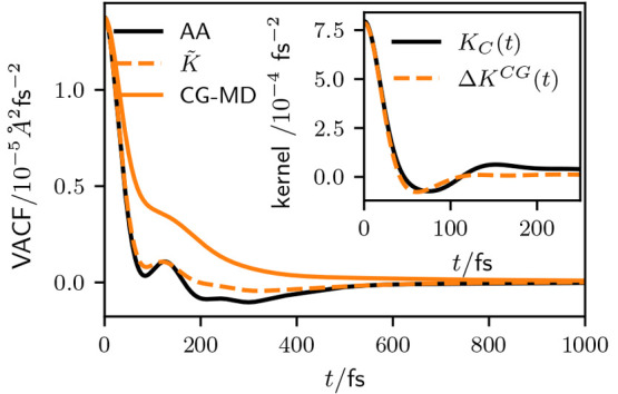
VACFs of the IBI water model, parametrized with K̃(t) (eq 15) calculated based on the BOD method, compared to the AA reference. For comparison we also show the result of nondissipative CG-MD simulations. Inset shows the memory kernel contribution K_C(t) from the reference simulation compared to the memory due to conservative interactions (ΔK^CG(t)) in CG GLE simulations parametrized with K̃(t).

The main assumption of the applied parametrization scheme lies in eq 14. In the inset of Figure 1, we show that K_C(t) from the reference model and ΔK^CG(t) from the CG GLE simulation indeed coincide very well on short time scales, but K_C(t) exhibits a long positive tail, which is not captured by ΔK^CG(t). This explains the residual deviations in the VACF on longer time scales. If eq 14 would strictly hold, the target VACF would trivially match exactly. Still, combined with the results of earlier studies,^19,20 the overall well match between K_C(t) and ΔK^CG(t) underscores the general soundness of the applied approach, at least as an a priori approximation.

The origin of the residual deviations can generally be 2-fold. First, at t = 0, both K_C(t) and ΔK^CG(t) are proportional to the variance of the CG conservative forces acting upon a CG DoF. This variance is determined by the CG potential and the sampled configurations. As the same CG potential in determining K_C(t) and ΔK^CG(t) is used, deviations at t = 0 can only arise due to deviations in the static structure between the AA reference and the CG model. Second, on long time scales, the EoM given by eq 1 poses inherent limitations, as the noise and friction on any CG DoF is modeled independently. In reality, the CG DoFs exchange momentum via the neglected DoFs, which cannot be captured in terms of eq 1. This, in turn, can affect the structural relaxation, which respectively induces deviations in ΔK^CG(t). Any deviation at times t > 0 cannot be exactly assigned to one of the two mechanisms, except for well-controlled model systems.²⁰

Still, despite these limitations, we find that this approach yields good results in conjunction with the IBI potential, without additional optimization of the parametrization.

Dynamics of the Iteratively Optimized IBI Model

Residual deviations of CG models from the AA reference due to the inherent approximations of the pure bottom-up approach can be reduced by iterative optimization of the parametrization of the GLE thermostat. Here, we apply the iterative optimization schemes (IOMK, IMRV-1, and IMRV-2) to optimize the parametrization of the memory kernel for the IBI model. But first, to justify the IOMK method given by eq 17, we will demonstrate the validity of the assumption given by eq 16. To do so, we performed CG simulations using the IBI potential by applying a Markovian Langevin thermostat with varying friction coefficients (γ_lang). By evaluating the integrated memory added through conservative interactions (ΔG^CG(t) = ∫₀^t ds ΔK^CG(s)), eq 16 can be tested.

In Figure 2, we show the result of this analysis. We find that the friction due to conservative interactions does span over a full order of magnitude for the tested values of γ_lang. The relationship between ΔG^CG(t = 10 ps) and γ_lang is found to be well-described by the linear fit

18

where a can be interpreted as the single-particle friction coefficient in standard CG-MD simulations in the absence of a Langevin thermostat and b encodes the dependence of the friction due to conservative interactions on the friction coefficient applied through the thermostat. For the IOMK method, we extrapolate this finding to eq 16, assuming that the linear relation holds true on all time scales.

Figure 2.

Friction introduced by conservative interactions in NVT simulations using a Langevin thermostat, as a function of the applied friction coefficient. The data shown are based on simulations of the IBI model. An almost-perfect linear dependence is found, which is emphasized by the linear fit, shown as a black dotted line.

In Figure 3, we compare the results of the three iterative schemes, while starting from G̃₀(t) = G̃(t) = ∫₀^t dsK̃(s) as an initial guess. We first note that the IMRV-1 method does not yield any significant improvement in the representation of the VACF, while the IMRV-2 method allows one to achieve good results. This is consistent with the findings in the original publication.¹⁶ The IOMK method yields satisfying results within 2–3 iterations, while the IMRV-2 method requires ∼30–40 iterations to match the target.

Figure 3.

Results for iterative optimization of memory kernels for the IBI water model. (a, b, c) Comparison of the VACF for the IOMK method (panel (a)), the IMRV-1 method (panel (b)), and the IMRV-2 method (panel (c)). (d–f) Comparison of D(t) = ∫₀^t dsC_VV(s) for the IOMK method (panel (d)), the IMRV-1 method (panel (e)), and the IMRV-2 method (panel (f)).

This indicates that the IOMK method converges fast, compared to the IMRV-2 method. To further test the reliability of the IOMK method, we also applied two different initial guesses: G̃₀(t) = ∫₀^t dsC_δF δF(s)/k_BT and G̃₀(t) = 0.1 ∫₀ dsC_δF δF(s)/k_BT. These data are presented in Figures S13 and S14 in the SI. In the former case, the initial guess slightly overestimates optimal friction, yielding too slow dynamics. Herein, the IOMK method converges within 3–4 iterations, while the IMRV-2 method requires ten times more iterations. In the latter case, the initial guess strongly underestimates the optimal friction, yielding too fast dynamics. Here, the IOMK method also converges within 3–4 steps, while the IMRV-2 method again requires ten times more iterations. For the presented system, the IOMK method is shown to be very stable and fast-converging, independent of the initial guess for the memory kernel.

Structural Relaxation: The Distinct Van Hove Function

Both the bottom-up parametrization approach and the IOMK method are motivated by the goal to match dynamic properties of single particles. No information on multibody correlations are considered in the parametrization of the memory kernels. Thus, it is not a priori clear inhowfar collective dynamic properties involving multiple particles can be captured by applying independent thermostatting to every CG DoF, as, e.g., interparticle correlations can be altered due to the independent thermostatting of every DoF.²⁰ In this section, we want to study the collective dynamics of the CG systems by evaluating the distinct VHF,

19

In Figure 4, we compare the distinct VHF of the IBI water model with standard CG-MD, the GLE with K̃(t) and the GLE optimized using the IOMK method. In CG-MD simulations without a GLE thermostat, structural correlations relax faster than in the AA reference. Especially in the short distance region, the value of the VHF increases too fast, which is expected, since, with an increased diffusivity, a particle can be more readily displaced and, consequently, be replaced by its neighbors. Additionally, we also find that the pair structure, especially the first peak, relaxes faster than in the AA reference. By introducing friction through the GLE thermostat, the structural relaxation is slowed and the pair structure is preserved for longer time scales. The K̃ model overall reproduces the VHF quite accurately at least up to 400 fs. The increased long time diffusivity of the K̃ model compared to the AA reference on short length scales leads to an acceleration in the relaxation beyond 400 fs. The optimization of the memory kernel through the IOMK method does not significantly alter the VHF for the first peak, but by matching the long-time diffusivity, the relaxation on short length scales is better reproduced.

Figure 4.

Distinct VHF for (a) the AA reference, (b) the CG-MD IBI model, (c) the K̃-model, and (d) the IOMK model.

In Figure 5a, we present a slice through the VHFs at R = 0.276 nm for a better time resolution of the relaxation of the first peak. Here, we see more clearly that the VHF decays too fast for CG-MD, which is improved with the GLE thermostat for both the K̃ model and the IOMK model. We additionally present the result of a Markovian Langevin-thermostat model, in which we optimized the friction coefficient such the diffusivity matches the AA reference. Herein, we find that, in such a Markovian model, the relaxation of the pair structure is too slow.

Figure 5.

Distinct VHF at (a) R = 0.276 nm and (b) R = 0.2 nm, for different CG IBI models, compared to the AA reference.

In Figure 5b, we present a slice through the VHF at R = 0.2 nm, where we again find that the CG-MD model yields too fast relaxation. On short time scales, both the K̃ model and the IOMK model match the reference significantly better, while the Markovian model again relaxes too slowly. On long time scales, the K̃-model relaxes too fast, while the AA reference, the IOMK model, and the Markovian model converge onto each other.

Comparison of the Different CG Water Models

Until now, we have only discussed the dynamics of IBI water models. We have shown that the purely bottom-up informed approach allows a semiquantative representation of the reference dynamics, while the IOMK method allows one to reproduce the VACF quantitatively, while also the representation of collective dynamics, in terms of the distinct VHF, is significantly improved.

In this section, we will compare how the choice of the CG potential influences the dynamic properties of purely bottom-up informed water models. The properties of the memory kernel contributions for the different conservative potentials are shown and discussed in Figure S4 in the SI.

Dynamics of Generalized Langevin Models

In this section, we study the dynamics of the different CG water models by applying a GLE thermostat. The VACFs for the two-body and three-body models are shown in Figures 6a and 6b, respectively. In Figure 6b, only the SW-FM model is considered, since, for the SW-RE model, the bottom-up approach predicts a nonphysical memory kernel K̃(t) (see Section S6 in the SI for a discussion on the origin of this behavior). We also studied GLE models parametrized with K_δ,X(t) = K_δ(t) + K_X(t) and K_δ(t), to study the relevance of the cross-correlation term K_X(t). Note that K_δ,X(t) is equivalent to a memory kernel which can be evaluated from a Volterra equation derived from eq 1(19) and has been proposed as a straightforward parametrization for both Markovian Langevin¹¹ and non-Markovian GLE thermostats.²¹ Using K_δ(t), thus neglecting cross-correlations all together, can be understood as a non-Markovian variant of the approach proposed in ref (14). The data on these models can be found in Figures S6 and S7 in the SI.

Figure 6.

VACFs from GLE simulations of CG models with a) two-body potentials b) three-body potentials, parametrized with K̃(t), compared to the AA reference.

In all shown cases in Figure 6, the GLE model yields a significant improvement of the representation of the reference dynamics, when compared to the standard CG-MD simulations (Figure S5 in the Supporting Information). The FM model cannot fully capture the fast initial decay of the VACF. The SW-FM model and the IBI model captures the initial decay quantitatively. The local features around 75–150 fs are qualitatively well-matched for the IBI models and the SW-FM models, while the depth of the broad negative valley 200–300 fs is underestimated in all cases, indicating again too fast overall mobility.

A comparison of K_C(t) and ΔK^CG(t) (as shown in the insets of Figures 6a and 6b) again reveals the origin of the remaining discrepancies. In the FM model, the onset of the memory kernel due to conservative forces in CG simulations is lower than K_C(t) would predict. This is due to mismatch of the pair structure in the FM model, which yields a reduction in the variance of conservative forces. This discrepancy on short time scales leads to the too slow initial decay on small time scales. Also the valley of K_C(t) is not as well reproduced as in the IBI model, leading to larger discrepancies in the VACF on similar time scales. For the SW-FM model, the assumption of eq 14 is well-justified up to 100 fs.

In all cases, the overall mobility is overpredicted with K̃(t). The origin trivially arises from deviation from the assumption of eq 14.

In addition to the bottom-up approach, we also applied the IOMK method to optimize the parametrization of the SW-FM and the SW-RE model. We find that the IOMK method can also be successfully applied to optimize the memory kernels in SW-type models. Figure 7 shows an overview over all studied CG models, by defining an error measure as

20

with N = 1000 and Δt = 2 fs.

Figure 7.

Error estimate of the VACF based on eq 20, for all CG simulations.

For the pure bottom-up approach, K̃(t) yields the best results for both CG pair potentials while K_δ,X(t) yields better results for the three-body potentials.

Structural Relaxation

We calculated the distinct VHF for all combinations of CG potentials and GLE thermostat parametrizations. A prerequisite for reproducing the VHF on all time scales is that the static pair structure is reproduced. Because the FM model does not reproduce the static pair structure (see Figure S3 in the SI), we only consider the IBI, SW-FM, and SW-RE models in this section. Additionally, to single out the influence of the choice of the CG potential, we first consider the simulations optimized through the IOMK method. This allows one to study the influence of the CG potential on structural relaxation, given that the static structure and the single-particle dynamics is accurately represented. In Figure 8a, we show the VHF for the first peak for the described systems, compared to the AA reference. For the relaxation of the first peak, all three models match the AA almost quantitatively. Still, the SW-RE model matches the reference data best, which can be seen by amplifying the plot, as shown in the inset. A more significant deviation between the different models is found for shorter length scales (R = 0.2 nm) in Figure 8b. Here, the IBI model deviates significantly from the AA reference, while both SW-type models reproduce the structural relaxation almost quantitatively.

Figure 8.

VHF for the IOMK models with the IBI, the SW-FM and the SW-RE model, compared to the AA reference, for (a) R = 0.276 nm and (b) R = 0.2 nm.

To compare the performance of all different combinations of CG potentials and thermostats, we define the error measure as

21

where N_i and N_j are the considered number of distance bins and time steps, respectively, R₀ is the minimal considered distance, δR is the bin width, and δt is the spacing is the resolution in time.

In Figure 9, we summarize the estimated deviations from the reference for the considered CG potentials for all thermostat parametrizations. This allows to draw the following conclusions:

• (1)In all cases, introducing a dissipative thermostat improves the representation of the VHF.
• (2)For the IBI potential, the IOMK model performs better than the Markovian model, while having the same diffusivity. One can conclude that matching the diffusivity is not sufficient to correctly model structural relaxation and memory effects must be taken into account.
• (3.For all CG potentials, the optimization of the VACF via the IOMK method leads to an improved representation of the VHF.
• (4)Given that the single-particle dynamics is well matched, as ensured by the IOMK method, and the static structure is well-reproduced, the representation of the structural relaxation is still dependent on the choice of the CG potential. The introduction of an angular potential for coarse-graining SPC/E water, improves, under the stated conditions, the representation of the VHF. Additionally, the SW-RE model performs better than the SW-FM model.

Figure 9.

Error estimate for the distinct VHF for all studied IBI, SW-FM, and SW-RE models.

Summary and Outlook

We have demonstrated that the previously proposed bottom-up approach for the parametrization of GLE thermostats based on the BOD method is applicable to molecular systems with complex interactions by coarse-graining SPC/E water, using effective single-site interactions. In conjunction with pairwise conservative interactions, the proposed parametrization of the GLE thermostat yields good results for most CG potentials. In particular, in accordance with previous studies,^19,20 taking into account the -projected cross-correlations is necessary to correctly reproduce the VACF on short time scales, and its neglect typically yields too slow dynamics. At the same time, we found that, for coarse-graining SPC/E water on a single interaction site, considering the cross-correlation term twice (using K̃(t) for the parametrization of the GLE thermostat) tends to overpredict the diffusivity. This is consistent with our findings in ref (20). and is due to the independent thermostatting of every CG DoF, which leads to a reduction of the correlation of the dynamics between different CG DoFs.

Using the example of the IBI potential, we have demonstrated the applicability of the IOMK method to optimize the VACF for molecular liquids and have demonstrated its stability and good convergence properties compared to previously proposed iterative optimization schemes. Our results indicate that the IOMK method converges fast, even when the initial guess is far from optimal. An additional benefit, compared to other methods, is that the IOMK method does not rely on any parameters that have to be manually predetermined to improve convergence behavior, which significantly increases its applicability as an out of the box tool for dynamic coarse-graining.

By studying the distinct VHF, we have demonstrated that, despite the conceptional limitation of an isotropic and configuration-independent thermostat, the application of a GLE thermostat in CG models allows one to model structural relaxation quite accurately. This is a nontrivial finding, as nowhere in the parametrization process collective dynamics is considered and indicates that a faithful connection to the underlying AA reference can be established under certain conditions. Of course, the prerequisite is that at least the pair structure is well-reproduced by the CG potential. By comparing the pairwise IBI potential with two three-body Stillinger-Weber type potentials (SW-FM and SW-RE) we found that an accurate representation of three-body correlations can further improve the accuracy of the distinct VHF, given an accurate representation of single-particle dynamics.

In principle, the choice of the target for the IOMK method is not limited to FG MD models. The single-particle memory kernel is accessible from the mean-squared displacement,⁵⁹ which by itself can be calculated from the self-part of the VHF from experiments.⁴⁷ This would allow to use the IOMK method in combination with top-down parametrized CG potentials, to improve the representation of dynamic properties in empirical CG models as for example the Molinero-Water model.⁶⁰ This would necessitate high quality experimental data with a high resolution in space and time, and methods to accurately extract the center of mass dynamics from experimental measurements. In practice such an approach has to to evaluated carefully, as it is unclear if current experimental data is sufficiently reliable to be used as quantitative reference. For example, the reported VHF in ref (48) does not quantitatively agree with earlier results in refs^{44, 45}.

In summary, we have shown that it is possible to derive good estimates of memory kernels in a purely bottom-up approach, which allow one to maintain a direct link between the parametrization of the GLE thermostat and the underlying AA reference. For the considered system, the bottom-up approach performs more reliably for CG pair potentials than for three-body potentials. Arguably, this is due to the increased complexity of the CG energy landscape, because, in such a case, even small discrepancies in the sampling of configuration space between AA and CG models can lead to significant errors in the prediction of memory due to conservative forces. The IOMK method allows to efficiently circumvent these issues by allowing to derive CG models which exactly reproduce the single-particle dynamics. Our results indicate that also collective dynamics can be accurately described by applying optimized memory kernels as long as the CG potential accurately reproduces the pair structure.

Methods

All-Atom Water Simulations

As a FG reference, we consider atomistic water under ambient conditions, applying the SPC/E model.⁶¹ The atomistic simulations were performed with the GROMACS package,^62,63 using a time step of 2 fs integrated via the velocity Verlet method. We use a cutoff of 1.2 nm for short-range van der Waals and electrostatic interactions and long-range dispersion corrections for energy and pressure. Long-range electrostatic interactions are treated with the particle mesh Ewald method with a grid spacing of 0.12 nm. The reference system was set up by preparing a cubic simulation box with 3000 water molecules. The box was equilibrated under NPT conditions at 1 bar and 298 K using the velocity-rescale thermostat with a time constant of 1 ps and the Berendsen barostat with a time constant 2 ps and compressibility parameter of experimental water of 4.5 × 10^–5 bar^–1. The average box-length of a NPT simulation was chosen to fix the box length to 4.47934 nm for further simulations.

For the evaluation of structural properties (the radial distribution function, RDF), an NVT run was performed for 200 ps. Snapshots were stored every 20 fs. To efficiently obtain sufficiently uncorrelated snapshots, a stochastic dynamics integrator was applied with a time constant of 1 ps.

For the evaluation of dynamic properties (VACF, memory kernels, distinct VHF), 10 independent NVE simulations were determined from different initial conditions drawn from a sample of NVT snapshots. Here, every run was performed for 50 ps, using the velocity Verlet integrator. Frames were stored every time step.

CG Simulations

We derived all tabular CG pair potentials using the VOTCA-CSG³⁵ package. We applied a center of mass mapping scheme for the CG representation.

For the IBI model, we set a cutoff distance of 1 nm for the CG pair potential. For every IBI iteration, simulations were performed for 120 ps under NVT conditions, using the stochastic integrator with a time constant of 0.5 ps. Snapshots for the evaluation of the RDF were taken every 20 fs. We stopped the optimization process after 300 iterations. For the derivation of the FM potential, we set the range of the potential to 0.24–0.9 nm, with a spacing of 0.012 nm. The three-body SW-type potentials were obtained from the literature. (See ref (37) for details on the SW-FM potential and ref (53) for details on the SW-RE potential.)

CG simulations were performed using the LAMMPS package.⁶⁴ All CG simulations were performed under NVT conditions, with 3000 CG beads, at 298 K, a box length of 4.47934 nm, and a time step of 2 fs.

For every CG system, we generated ten 20-ps trajectories. Dynamic properties were evaluated for every distinct trajectory, and values were averaged to reduce statistical uncertainty.

For standard CG-MD simulations the Nosé–Hoover thermostat was applied with a time constant of 2000 fs. For GLE simulations, the GLE thermostat due to Ceriotti⁶⁵ was applied. This thermostat is based on an auxiliary variable approach, which allows one to simulate non-Markovian dynamics by applying a Markovian EoM in extended phase space. For its application in the context of CG, the coupling between the CG momenta and the auxiliary momenta must be defined in terms of a coupling matrix. This matrix can be determined from a given memory kernel, by fitting with exponentially dampened oscillators. For all CG GLE models, we chose to fit six exponentially dampened oscillators, yielding 12 auxiliary momenta for the Markovian embedding. In practice we fitted the integrals of the memory kernels. For all BOD method based parametrizations the memory kernels were fitted up to t = 800 fs. For the IOMK method, we fitted the memory kernels up to t = 2000 fs, to better capture the hydrodynamic tail of the VACF. Further details on the Markovian embedding of GLEs can be found in our earlier publications^7,20 or, for example, in refs (15), (25), (66), and (67).

Bottom-Up Derivation of Memory Kernels from Backward-Orthogonal Dynamics

Details on the BOD method can be found in refs (19), (20), (43), and (57), so we will only shortly summarize the overall workflow. The first step is always to perform FG (AA) simulations, where frames are stored sufficiently frequently (every time step in the current work) to reduce numerical errors in the BOD method. Both velocities and total forces for every DoF must be stored. Next, we apply the center of mass mapping on the AA trajectory (using the VOTCA-CSG software³⁵) to obtain a mapped reference trajectory. Based on this mapped trajectory, a rerun is performed using the required CG potential to obtain a trajectory for the conservative interactions F_I^C(t), which, through δF_I(t) = F_I (t) – F_I(t) also yield a time series for the residual forces. From the time series of F_I(t), F_I^C(t), δF_I(t), and V_I(t), the respective force-correlation functions can be obtained applying the BOD method. As a numerical scheme, we utilize the second-order scheme proposed by Jung et al.^19,20,43

The IMRV Method

The update scheme for the IMRV-1 method and the IMRV-2 method is given by

22

The update function Δϕ_i(t) is given by

23

where the superscript “tgt” denotes the target function and the subscript “i” denotes the current iteration. For IMRV-1, the function ϕ_i(t) is defined by the respective VACF C_VV,i(t) as

24

and analogously for ϕ^tgt(t). The function h_i(t) defines the step size for the iterations and can be tuned to improve the stability of the scheme. Jung et al.⁴³ proposed

25

The IMRV-2 method defines a different function ϕ_i(t) (and, accordingly, ϕ^tgt(t)), which reads¹⁶

26

Note that, for the IMRV2 method, an additional constant α must be set. After manual optimization, we applied t_corr = 80 fs and α = 0.05 fs^–1.

Data Availability Statement

The data that supports the findings of this study are available within the article and its supplementary material. At https://doi.org/10.48328/tudatalib-937 we provide all results (memory kernels, VACFS etc.) as text files. We also provide input data for the AA model and the CG models discussed in this work including tabular potentials and the coupling matrices for the application of the auxiliary variable GLE thermostat. At https://github.com/vklip/IOMK we provide a minimal working example for the application of the IOMK method to derive optimized GLE thermostat models, based on the IBI potential. An implementation of the IOMK method within the VOTCA software will be developed at https://github.com/vklip/votca-iomk.

Supporting Information Available

The Supporting Information is available free of charge at https://pubs.acs.org/doi/10.1021/acs.jctc.2c00871.

• Discussion of the relation of the IOMK and the IMRV-2 to the Newton method; presentation of most of the data shown in the main text, alongside the results for two additional CG potentials, which is an IBI potential where we applied a pressure ramp (IBI-p) and the well-known SW-type model due to Molinero et al.⁶⁰ (MW); CG pair potentials derived for this study (Figure S2); comparison of the structure (in terms of the RDF and the angular distribution function) of all CG water models with SPC/E water (Figure S3); memory kernels derived from the BOD-method and, where applicable, the optimized IOMK memory kernels (Figure S4); VACFs from CG-MD simulations for all CG potentials (Figure S5); VACFs from CG GLE thermostat simulations, including parametrizations of the GLE thermostat with K_δ(t) and K_δ,X(t) = K_δ(t) + K_X(t) (Figures S6–S8); memory due to conservative interactions in the SW-RE and the MW model to the predictions (K_C(t)) due to the BOD-method, to demonstrate why for these models a meaningful parametrization of the GLE thermostat, using K̃(t) is not possible (Figure S9); VACFs and the corresponding integrals (D(t) = ∫₀^t dsC_VV(s)) to compare long time diffusion coefficients (Figure S10); the modeling errors of all CG models, including the IBI-p and the MW models (Figure S11); visualization of the convergence of the IOMK, IMRV-1, and IMRV-2 methods (Figure S12); results for the IOMK and IMRV-2 method with alternative initial guesses (Figures S13 and S14); results for the IOMK method for the SW-type potentials (Figures S15–S17); all VHFs (Figures S18–S29); and a summary of the modeling errors of the VHFs for all models, including the results for the IBI-p and MW models (Figure S30) (PDF)

Funded by the Deutsche Forschungsgemeinschaft (DFG, German Research Foundation), Project No. 233630050-TRR 146.

The authors declare no competing financial interest.

References

- Müller-Plathe F. Coarse-Graining in Polymer Simulation: From the Atomistic to the Mesoscopic Scale and Back. ChemPhysChem 2002, 3, 754–769. . [DOI] [PubMed] [Google Scholar]
- Noid W. G. In Biomolecular Simulations: Methods and Protocols; Monticelli L., Salonen E., Eds.; Methods in Molecular Biology, Vol. 924; Humana Press: Totowa, NJ, 2013; pp 487–531. [DOI] [PubMed] [Google Scholar]
- Dhamankar S.; Webb M. A. Chemically Specific Coarse-Graining of Polymers: Methods and Prospects. J. Polym. Sci. 2021, 59, 2613–2643. 10.1002/pol.20210555. [DOI] [Google Scholar]
- Brini E.; Algaer E. A.; Ganguly P.; Li C.; Rodríguez-Ropero F.; van der Vegt N. F. A. Systematic Coarse-Graining Methods for Soft Matter Simulations-a Review. Soft Matter 2013, 9, 2108–2119. 10.1039/C2SM27201F. [DOI] [Google Scholar]
- Fritz D.; Koschke K.; Harmandaris V. A.; van der Vegt N. F. A.; Kremer K. Multiscale Modeling of Soft Matter: Scaling of Dynamics. Phys. Chem. Chem. Phys. 2011, 13, 10412–10420. 10.1039/c1cp20247b. [DOI] [PubMed] [Google Scholar]
- Rudzinski J. F. Recent Progress towards Chemically-Specific Coarse-Grained Simulation Models with Consistent Dynamical Properties. Computation 2019, 7, 42. 10.3390/computation7030042. [DOI] [Google Scholar]
- Klippenstein V.; Tripathy M.; Jung G.; Schmid F.; van der Vegt N. F. A. Introducing Memory in Coarse-Grained Molecular Simulations. J. Phys. Chem. B 2021, 125, 4931–4954. 10.1021/acs.jpcb.1c01120. [DOI] [PMC free article] [PubMed] [Google Scholar]
- Meinel M. K.; Müller-Plathe F. Loss of Molecular Roughness upon Coarse-Graining Predicts the Artificially Accelerated Mobility of Coarse-Grained Molecular Simulation Models. J. Chem. Theory Comput. 2020, 16, 1411–1419. 10.1021/acs.jctc.9b00943. [DOI] [PubMed] [Google Scholar]
- Meinel M. K.; Müller-Plathe F. Roughness Volumes: An Improved RoughMob Concept for Predicting the Increase of Molecular Mobility upon Coarse-Graining. J. Phys. Chem. B 2022, 126, 3737–3747. 10.1021/acs.jpcb.2c00944. [DOI] [PubMed] [Google Scholar]
- Akkermans R. L.; Briels W. J. Coarse-Grained Dynamics of One Chain in a Polymer Melt. J. Chem. Phys. 2000, 113, 6409–6422. 10.1063/1.1308513. [DOI] [Google Scholar]
- Izvekov S.; Voth G. A. Modeling Real Dynamics in the Coarse-Grained Representation of Condensed Phase Systems. J. Chem. Phys. 2006, 125, 151101. 10.1063/1.2360580. [DOI] [PubMed] [Google Scholar]
- Izvekov S. Mori-Zwanzig Theory for Dissipative Forces in Coarse-Grained Dynamics in the Markov Limit. Phys. Rev. E 2017, 95, 013303. 10.1103/PhysRevE.95.013303. [DOI] [PubMed] [Google Scholar]
- Hijón C.; Español P.; Vanden-Eijnden E.; Delgado-Buscalioni R. Mori–Zwanzig Formalism as a Practical Computational Tool. Faraday Discuss. 2010, 144, 301–322. 10.1039/B902479B. [DOI] [PubMed] [Google Scholar]
- Lei H.; Caswell B.; Karniadakis G. E. Direct Construction of Mesoscopic Models from Microscopic Simulations. Phys. Rev. E 2010, 81, 026704. 10.1103/PhysRevE.81.026704. [DOI] [PMC free article] [PubMed] [Google Scholar]
- Li Z.; Lee H. S.; Darve E.; Karniadakis G. E. Computing the Non-Markovian Coarse-Grained Interactions Derived from the Mori-Zwanzig Formalism in Molecular Systems: Application to Polymer Melts. J. Chem. Phys. 2017, 146, 014104. 10.1063/1.4973347. [DOI] [PubMed] [Google Scholar]
- Jung G.; Hanke M.; Schmid F. Generalized Langevin Dynamics: Construction and Numerical Integration of Non-Markovian Particle-Based Models. Soft Matter 2018, 14, 9368–9382. 10.1039/C8SM01817K. [DOI] [PubMed] [Google Scholar]
- Lemarchand C. A.; Couty M.; Rousseau B. Coarse-Grained Simulations of Cis- and Trans-Polybutadiene: A Bottom-up Approach. J. Chem. Phys. 2017, 146, 074904. 10.1063/1.4975652. [DOI] [PubMed] [Google Scholar]
- Deichmann G.; van der Vegt N. F. A. Bottom-up Approach to Represent Dynamic Properties in Coarse-Grained Molecular Simulations. J. Chem. Phys. 2018, 149, 244114. 10.1063/1.5064369. [DOI] [PubMed] [Google Scholar]
- Klippenstein V.; van der Vegt N. F. A. Cross-Correlation Corrected Friction in (Generalized) Langevin Models. J. Chem. Phys. 2021, 154, 191102. 10.1063/5.0049324. [DOI] [PubMed] [Google Scholar]
- Klippenstein V.; van der Vegt N. F. A. Cross-Correlation Corrected Friction in Generalized Langevin Models: Application to the Continuous Asakura-Oosawa Model. J. Chem. Phys. 2022, 157, 044103. 10.1063/5.0093056. [DOI] [PubMed] [Google Scholar]
- Han Y.; Dama J. F.; Voth G. A. Mesoscopic Coarse-Grained Representations of Fluids Rigorously Derived from Atomistic Models. J. Chem. Phys. 2018, 149, 044104. 10.1063/1.5039738. [DOI] [PubMed] [Google Scholar]
- Han Y.; Jin J.; Voth G. A. Constructing Many-Body Dissipative Particle Dynamics Models of Fluids from Bottom-up Coarse-Graining. J. Chem. Phys. 2021, 154, 084122. 10.1063/5.0035184. [DOI] [PubMed] [Google Scholar]
- Markutsya S.; Lamm M. H. A Coarse-Graining Approach for Molecular Simulation That Retains the Dynamics of the All-Atom Reference System by Implementing Hydrodynamic Interactions. J. Chem. Phys. 2014, 141, 174107. 10.1063/1.4898625. [DOI] [PubMed] [Google Scholar]
- Stoffel T. D.; Haskins J. B.; Lawson J. W.; Markutsya S. Coarse-Grained Dynamically Accurate Simulations of Ionic Liquids: [Pyr14][TFSI] and [EMIM][BF4]. J. Phys. Chem. B 2022, 126, 1819–1829. 10.1021/acs.jpcb.1c08107. [DOI] [PubMed] [Google Scholar]
- Wang S.; Ma Z.; Pan W. Data-Driven Coarse-Grained Modeling of Polymers in Solution with Structural and Dynamic Properties Conserved. Soft Matter 2020, 16, 8330–8344. 10.1039/D0SM01019G. [DOI] [PubMed] [Google Scholar]
- Davtyan A.; Dama J. F.; Voth G. A.; Andersen H. C. Dynamic Force Matching: A Method for Constructing Dynamical Coarse-Grained Models with Realistic Time Dependence. J. Chem. Phys. 2015, 142, 154104. 10.1063/1.4917454. [DOI] [PubMed] [Google Scholar]
- Davtyan A.; Voth G. A.; Andersen H. C. Dynamic Force Matching: Construction of Dynamic Coarse-Grained Models with Realistic Short Time Dynamics and Accurate Long Time Dynamics. J. Chem. Phys. 2016, 145, 224107. 10.1063/1.4971430. [DOI] [PubMed] [Google Scholar]
- Zwanzig R.Nonequilibrium Statistical Mechanics; Oxford University Press, 2001. [Google Scholar]
- Gao L.; Fang W. Semi-Bottom-up Coarse Graining of Water Based on Microscopic Simulations. J. Chem. Phys. 2011, 135, 184101. 10.1063/1.3658500. [DOI] [PubMed] [Google Scholar]
- Deichmann G.; Marcon V.; van der Vegt N. F. A. Bottom-up Derivation of Conservative and Dissipative Interactions for Coarse-Grained Molecular Liquids with the Conditional Reversible Work Method. J. Chem. Phys. 2014, 141, 224109. 10.1063/1.4903454. [DOI] [PubMed] [Google Scholar]
- Li Z.; Bian X.; Caswell B.; Karniadakis G. E. Construction of Dissipative Particle Dynamics Models for Complex Fluids via the Mori-Zwanzig Formulation. Soft Matter 2014, 10, 8659–8672. 10.1039/C4SM01387E. [DOI] [PubMed] [Google Scholar]
- Li Z.; Bian X.; Li X.; Karniadakis G. E. Incorporation of Memory Effects in Coarse-Grained Modeling via the Mori-Zwanzig Formalism. J. Chem. Phys. 2015, 143, 243128. 10.1063/1.4935490. [DOI] [PMC free article] [PubMed] [Google Scholar]
- Glatzel F.; Schilling T. The Interplay between Memory and Potentials of Mean Force: A Discussion on the Structure of Equations of Motion for Coarse Grained Observables. Europhys. Lett. 2021, 136, 36001. 10.1209/0295-5075/ac35ba. [DOI] [Google Scholar]
- Izvekov S.; Voth G. A. Multiscale Coarse Graining of Liquid-State Systems. J. Chem. Phys. 2005, 123, 134105. 10.1063/1.2038787. [DOI] [PubMed] [Google Scholar]
- Rühle V.; Junghans C.; Lukyanov A.; Kremer K.; Andrienko D. Versatile Object-Oriented Toolkit for Coarse-Graining Applications. J. Chem. Theory Comput. 2009, 5, 3211–3223. 10.1021/ct900369w. [DOI] [PubMed] [Google Scholar]
- Lyubartsev A.; Mirzoev A.; Chen L.; Laaksonen A. Systematic Coarse-Graining of Molecular Models by the Newton Inversion Method. Faraday Discuss. 2010, 144, 43–56. 10.1039/B901511F. [DOI] [PubMed] [Google Scholar]
- Scherer C.; Andrienko D. Understanding Three-Body Contributions to Coarse-Grained Force Fields. Phys. Chem. Chem. Phys. 2018, 20, 22387–22394. 10.1039/C8CP00746B. [DOI] [PubMed] [Google Scholar]
- Scherer C.; Scheid R.; Andrienko D.; Bereau T. Kernel-Based Machine Learning for Efficient Simulations of Molecular Liquids. J. Chem. Theory Comput. 2020, 16, 3194–3204. 10.1021/acs.jctc.9b01256. [DOI] [PMC free article] [PubMed] [Google Scholar]
- Bernhardt M. P.; Hanke M.; van der Vegt N. F. A. Iterative Integral Equation Methods for Structural Coarse-Graining. J. Chem. Phys. 2021, 154, 084118. 10.1063/5.0038633. [DOI] [PubMed] [Google Scholar]
- Moradzadeh A.; Aluru N. R. Many-Body Neural Network-Based Force Field for Structure-Based Coarse-Graining of Water. J. Phys. Chem. A 2022, 126, 2031–2041. 10.1021/acs.jpca.1c09786. [DOI] [PubMed] [Google Scholar]
- Eriksson A.; Jacobi M. N.; Nyström J.; Tunstrøm K. Effective Thermostat Induced by Coarse Graining of Simple Point Charge Water. J. Chem. Phys. 2008, 129, 024106. 10.1063/1.2953320. [DOI] [PubMed] [Google Scholar]
- Eriksson A.; Jacobi M. N.; Nyström J.; Tunstrøm K. Bottom-up Derivation of an Effective Thermostat for United Atoms Simulations of Water. J. Chem. Phys. 2009, 130, 164509. 10.1063/1.3119922. [DOI] [PubMed] [Google Scholar]
- Jung G.; Hanke M.; Schmid F. Iterative Reconstruction of Memory Kernels. J. Chem. Theory Comput. 2017, 13, 2481–2488. 10.1021/acs.jctc.7b00274. [DOI] [PubMed] [Google Scholar]
- Iwashita T.; Wu B.; Chen W.-R.; Tsutsui S.; Baron A. Q. R.; Egami T. Seeing Real-Space Dynamics of Liquid Water through Inelastic X-ray Scattering. Sci. Adv. 2017, 3, e1603079 10.1126/sciadv.1603079. [DOI] [PMC free article] [PubMed] [Google Scholar]
- Shinohara Y.; Dmowski W.; Iwashita T.; Wu B.; Ishikawa D.; Baron A. Q. R.; Egami T. Viscosity and Real-Space Molecular Motion of Water: Observation with Inelastic x-Ray Scattering. Phys. Rev. E 2018, 98, 022604. 10.1103/PhysRevE.98.022604. [DOI] [PubMed] [Google Scholar]
- Shinohara Y.; Dmowski W.; Iwashita T.; Ishikawa D.; Baron A. Q. R.; Egami T. Local Correlated Motions in Aqueous Solution of Sodium Chloride. Physical Review Materials 2019, 3, 065604. 10.1103/PhysRevMaterials.3.065604. [DOI] [Google Scholar]
- Shinohara Y.; Dmowski W.; Iwashita T.; Ishikawa D.; Baron A. Q. R.; Egami T. Local Self-Motion of Water through the Van Hove Function. Phys. Rev. E 2020, 102, 032604. 10.1103/PhysRevE.102.032604. [DOI] [PubMed] [Google Scholar]
- Matsumoto R. A.; Thompson M. W.; Vuong V. Q.; Zhang W.; Shinohara Y.; van Duin A. C. T.; Kent P. R. C.; Irle S.; Egami T.; Cummings P. T. Investigating the Accuracy of Water Models through the Van Hove Correlation Function. J. Chem. Theory Comput. 2021, 17, 5992–6005. 10.1021/acs.jctc.1c00637. [DOI] [PubMed] [Google Scholar]
- Noid W. G.; Chu J.-W.; Ayton G. S.; Krishna V.; Izvekov S.; Voth G. A.; Das A.; Andersen H. C. The Multiscale Coarse-Graining Method. I. A Rigorous Bridge between Atomistic and Coarse-Grained Models. J. Chem. Phys. 2008, 128, 244114. 10.1063/1.2938860. [DOI] [PMC free article] [PubMed] [Google Scholar]
- Reith D.; Pütz M.; Müller-Plathe F. Deriving Effective Mesoscale Potentials from Atomistic Simulations. J. Comput. Chem. 2003, 24, 1624–1636. 10.1002/jcc.10307. [DOI] [PubMed] [Google Scholar]
- Stillinger F. H.; Weber T. A. Computer Simulation of Local Order in Condensed Phases of Silicon. Phys. Rev. B 1985, 31, 5262–5271. 10.1103/PhysRevB.31.5262. [DOI] [PubMed] [Google Scholar]
- Shell M. S. The Relative Entropy Is Fundamental to Multiscale and Inverse Thermodynamic Problems. J. Chem. Phys. 2008, 129, 144108. 10.1063/1.2992060. [DOI] [PubMed] [Google Scholar]
- Lu J.; Qiu Y.; Baron R.; Molinero V. Coarse-Graining of TIP4P/2005, TIP4P-Ew, SPC/E, and TIP3P to Monatomic Anisotropic Water Models Using Relative Entropy Minimization. J. Chem. Theory Comput. 2014, 10, 4104–4120. 10.1021/ct500487h. [DOI] [PubMed] [Google Scholar]
- Schilling T. Coarse-Grained Modelling Out of Equilibrium. Phys. Rep. 2022, 972, 1. 10.1016/j.physrep.2022.04.006. [DOI] [Google Scholar]
- te Vrugt M.; Wittkowski R. Projection Operators in Statistical Mechanics: A Pedagogical Approach. Eur. J. Phys. 2020, 41, 045101. 10.1088/1361-6404/ab8e28. [DOI] [Google Scholar]
- Straube A. V.; Kowalik B. G.; Netz R. R.; Höfling F. Rapid Onset of Molecular Friction in Liquids Bridging between the Atomistic and Hydrodynamic Pictures. Commun. Phys. 2020, 3, 126. 10.1038/s42005-020-0389-0. [DOI] [Google Scholar]
- Carof A.; Vuilleumier R.; Rotenberg B. Two Algorithms to Compute Projected Correlation Functions in Molecular Dynamics Simulations. J. Chem. Phys. 2014, 140, 124103. 10.1063/1.4868653. [DOI] [PubMed] [Google Scholar]
- Yoshimoto Y.; Li Z.; Kinefuchi I.; Karniadakis G. E. Construction of Non-Markovian Coarse-Grained Models Employing the Mori-Zwanzig Formalism and Iterative Boltzmann Inversion. J. Chem. Phys. 2017, 147, 244110. 10.1063/1.5009041. [DOI] [PubMed] [Google Scholar]
- Kowalik B.; Daldrop J. O.; Kappler J.; Schulz J. C. F.; Schlaich A.; Netz R. R. Memory-Kernel Extraction for Different Molecular Solutes in Solvents of Varying Viscosity in Confinement. Phys. Rev. E 2019, 100, 012126. 10.1103/PhysRevE.100.012126. [DOI] [PubMed] [Google Scholar]
- Molinero V.; Moore E. B. Water Modeled As an Intermediate Element between Carbon and Silicon. J. Phys. Chem. B 2009, 113, 4008–4016. 10.1021/jp805227c. [DOI] [PubMed] [Google Scholar]
- Berendsen H. J. C.; Grigera J. R.; Straatsma T. P. The Missing Term in Effective Pair Potentials. J. Phys. Chem. 1987, 91, 6269–6271. 10.1021/j100308a038. [DOI] [Google Scholar]
- Berendsen H.; van der Spoel D.; van Drunen R. GROMACS: A Message-Passing Parallel Molecular Dynamics Implementation. Comput. Phys. Commun. 1995, 91, 43–56. 10.1016/0010-4655(95)00042-E. [DOI] [Google Scholar]
- Abraham M. J.; Murtola T.; Schulz R.; Páll S.; Smith J. C.; Hess B.; Lindahl E. GROMACS: High Performance Molecular Simulations through Multi-Level Parallelism from Laptops to Supercomputers. SoftwareX 2015, 1–2, 19–25. 10.1016/j.softx.2015.06.001. [DOI] [Google Scholar]
- Thompson A. P.; Aktulga H. M.; Berger R.; Bolintineanu D. S.; Brown W. M.; Crozier P. S.; in ’t Veld P. J.; Kohlmeyer A.; Moore S. G.; Nguyen T. D.; Shan R.; Stevens M. J.; Tranchida J.; Trott C.; Plimpton S. J. LAMMPS - a Flexible Simulation Tool for Particle-Based Materials Modeling at the Atomic, Meso, and Continuum Scales. Comput. Phys. Commun. 2022, 271, 108171. 10.1016/j.cpc.2021.108171. [DOI] [Google Scholar]
- Ceriotti M.; Bussi G.; Parrinello M. Colored-Noise Thermostats à La Carte. J. Chem. Theory Comput. 2010, 6, 1170–1180. 10.1021/ct900563s. [DOI] [Google Scholar]
- Ceriotti M.; Bussi G.; Parrinello M. Langevin Equation with Colored Noise for Constant-Temperature Molecular Dynamics Simulations. Phys. Rev. Lett. 2009, 102, 20601. 10.1103/PhysRevLett.102.020601. [DOI] [PubMed] [Google Scholar]
- Wang S.; Li Z.; Pan W. Implicit-Solvent Coarse-Grained Modeling for Polymer Solutions via Mori-Zwanzig Formalism. Soft Matter 2019, 15, 7567–7582. 10.1039/C9SM01211G. [DOI] [PubMed] [Google Scholar]
Associated Data
This section collects any data citations, data availability statements, or supplementary materials included in this article.
Supplementary Materials