mRisk: Continuous Risk Estimation for Smoking Lapse from Noisy Sensor Data with Incomplete and Positive-Only Labels

Abstract

Passive detection of risk factors (that may influence unhealthy or adverse behaviors) via wearable and mobile sensors has created new opportunities to improve the effectiveness of behavioral interventions. A key goal is to find opportune moments for intervention by passively detecting rising risk of an imminent adverse behavior. But, it has been difficult due to substantial noise in the data collected by sensors in the natural environment and a lack of reliable label assignment of low- and high-risk states to the continuous stream of sensor data. In this paper, we propose an event-based encoding of sensor data to reduce the effect of noises and then present an approach to efficiently model the historical influence of recent and past sensor-derived contexts on the likelihood of an adverse behavior. Next, to circumvent the lack of any confirmed negative labels (i.e., time periods with no high-risk moment), and only a few positive labels (i.e., detected adverse behavior), we propose a new loss function. We use 1,012 days of sensor and self-report data collected from 92 participants in a smoking cessation field study to train deep learning models to produce a continuous risk estimate for the likelihood of an impending smoking lapse. The risk dynamics produced by the model show that risk peaks an average of 44 minutes before a lapse. Simulations on field study data show that using our model can create intervention opportunities for 85% of lapses with 5.5 interventions per day.

1. INTRODUCTION

Interventions delivered on a mobile device are an important tool to improve health and wellness via behavior change such as for smoking cessation. Decades of research in pharmacological and behavioral intervention methods have improved the success rate of quit attempts, but they still hover near 30% [33]. Knowing when the participant is at-risk of an adverse behavior can enable the exploration of whether and how well delivering targeted interventions at moments of risk can improve efficacy. For example, [49] presented a context-aware method to deliver timely interventions by sensing the exposure to geolocation-based smoking cues.

To detect the high-risk moments of an imminent adverse event, it is important to identify the dynamic risk factors that influence the occurrence of the adverse event. Prior research [38, 48, 66] has shown that these risk factors can be divided into two categories. First are the ‘external’ stimuli, i.e., environmental/social cues conducive to lapse (e.g., proximity to a bar or seeing others smoke may increase the risk of a smoking lapse). Second are the ‘internal’ stimuli such as stress or craving that may increase an individual’s vulnerability to lapse. Depletion of coping capacity during exposure to risk factors may result in a lapse.

Behavioral science suggests that just-in-time interventions, aiming to prevent a lapse, should adapt to both dynamically varying internal and external factors to provide optimal support at the right moment [48]. The emergence of sensors in wearables and smartphones has made it possible to passively detect dynamic changes in internal risk factors (e.g., stress [27, 58] and craving [8, 22]). Dynamic changes in the external risk factors for smoking lapse can also be detected passively using GPS and activity sensors (e.g., visits to smoking spots [9]). Deriving a composite risk score that reflects the dynamically varying levels of risk continuously can provide new opportunities to optimize both the timing and contents of interventions via micro-randomized trials [36].

Substantial work has been done in estimating risk scores for other kinds of adverse events. They include mortality [5, 19, 20, 71], ICU admission [79, 82], disease onset [2, 13, 18, 28, 78], fire hazard [43, 69, 73], flood [47], wildfire [21, 57], and road accidents [12, 44, 45]. The use of deep learning models helps obtain a composite risk score that encodes the underlying collective predictive power of all the input risk factors. For training and testing these models, carefully curated and labeled input data with timestamps of adverse event occurrences are used. All data not labeled to correspond to an adverse event are usually treated as negatively-labeled (i.e., low-risk). For example, when predicting mortality in ICU from large-scale electronic health records data (e.g., MIMIC-II), each of the 4,000 patients is either in the mortality (534 in Class 1) or the survival class (3,466 in Class 2) [5].

Estimating a composite risk score for adverse health-related behaviors poses three new challenges. First, continuous sensor data collected from wearables and smartphones to capture risk factors of adverse behaviors in the natural environment are usually noisy and incomplete [52]. This may be due to lack of firm attachment (e.g., proximity of pulse plethysmography (PPG) sensor to the skin in smartwatches that are used to detect stress and craving), intermittent noises (e.g., motion-induced deterioration of PPG data due to frequent wrist movements), and confounds (e.g., elevated physiology during recovery from physical activity may be confused with stress response). Second, for adverse behavioral events such as a smoking lapse, capturing the precise timing of each smoking lapse may not be feasible, as sensors may not be worn at the time of a lapse or the lapse events may not be accurately detected due to the imperfection of machine learning models that are used to detect smoking events via hand-to-mouth gestures [55]. Therefore, only a few positive events (i.e., smoking lapse in a cessation attempt) are available. Third, confirmed negative labels can be assigned to a block of sensor data corresponding to a prediction window only if the entire time period is confirmed to have no high-risk moment. As not all high-risk moments may result in a lapse, labeling a block of sensor data to the negative class is difficult for such events.

In this paper, we address each of the three challenges noted above. We first encode the noisy sensor data in the form of events that represent the psychological (e.g., stress), behavioral (e.g., activity), and environmental contexts (e.g., proximity to a smoking spot). Second, each of these contexts has substantial diversity in their representation (e.g., frequency, duration, type, etc.). We compute their homogeneous statistical representations to use them in training deep learning models. Third, we explore two approaches to succinctly capture the historical influence of recent and past events (i.e., substantial change in any context) to make deep learning models efficient. In the first approach called Deep Model with Recent Event Summarization (DRES), we summarize the influence of recent and past events via new features. In the second approach called Deep Model with Decaying Historical Influence (DDHI), we explicitly encode the influence of recent and past events as an exponentially decaying function over time. We refer to both models as mRisk model choices. Fourth, we address the challenge of sparse and positive-only labels via the Positive-Unlabeled (PU) framework, which allows for model training with positive-only labels. However, PU frameworks usually train models by giving higher weights to the positive samples and use a spy dataset (that has a small number of both positive and negative samples) for evaluation [41]. But, we do not have access to even such a small spy dataset. Therefore, we design a new loss function (called Rare Positive (RP)) to train the mRisk model choices and use the concept of the rarity of the positive class for evaluation.

We train and test the two models on a real-life smoking cessation dataset. We evaluate the performance of the two models via the risk characteristics they produce and their ability to create intervention opportunities prior to each confirmed smoking lapse moment. We find that 85% of lapses can be intervened upon with about 5.5 interventions per day. By analyzing the risk dynamics around lapse moments, we discover that risk usually peaks 44 minutes prior to a lapse. Finally, we use SHAP [42] to explain the influence of different contexts on lapse risk and find that recent visit to a smoking spot has the highest influence on risk, followed by stress.

2. SMOKING CESSATION STUDY AND DATA DESCRIPTION

We introduce smoking cessation, describe the smoking cessation study, and the resulting data used in modeling. The Institutional Review Board (IRB) approved the study, and all the participants provided written consent.

2.1. Smoking Cessation Research

Smoking is the leading preventable cause of mortality, causing 7 million deaths globally each year [1]. Therefore, extensive research has been done to support smoking cessation and to understand the smoking lapse process to improve rates of successful quitting. When a smoker attempts to quit smoking (i.e., abstain), withdrawal symptoms due to nicotine deprivation trigger several physiological and behavioral changes such as increase in stress, anxiety, concentration impairment, and craving [66, 67]. These changes can be further accentuated by certain situational or environmental influences such as exposure to smoking cues (e.g., proximity to a cigarette point of sale) or social triggers (e.g., drinks with friends) [53, 66]. These physiological and/or situational events constitute a high-risk situation for a smoking lapse. Individuals who are unable to cope with the acute challenges of high-risk situations, transition from abstinence to a smoking lapse [63]. In most cases, the first lapse eventually leads to full relapse [34, 65]. To capture risk factors for a smoking lapse that can be passively detected from wearable sensors and used for continuously estimating lapse risk, we conducted a new smoking cessation study.

2.2. Participants

Participants were recruited in a number of ways. First, recruitment flyers were posted in public areas such as college campuses, community clinics, churches, and in local restaurants and bars in Houston. Advertisements were placed in local newspapers and on radio. In person recruitment was implemented as needed to promote enrollment, or if requested by groups or institutions that have a population who is likely eligible and interested. The recruited participants went through the informed consent process during their initial (baseline) lab visit.

We use data from 170 enrolled participants (76 female), all 18+ years of age, with a mean age of 49.158 ± 12.99 years. All participants were African-American, residents of a city in the USA, smoked at least 3 cigarettes per day, and were motivated to quit smoking within the next 30 days of the start of the study. All of them agreed to wear the sensor suite. Participants were excluded if they had a contraindication for the nicotine patch (e.g., participants at risk of heart attack, angina, and other related health problems), active substance abuse or dependence issues, physically unable to wear equipment, pregnant or lactating, or currently using tobacco cessation medications.

2.3. Study Protocol

Interested participants were invited to an in-person information session where they were provided with detailed information about the study. Once enrolled at the baseline visit, participants picked a smoking quit date. They visited the lab during which they were trained in the proper use of the sensor devices and how to respond to questionnaires in the form of Ecological Momentary Assessments (EMA) via a study-provided smartphone. They wore the sensors for 4 days during the pre-quit phase.

On their set quit date, participants returned to the lab. Then they wore the sensors for 10 more days during the post-quit (or smoking cessation) phase. At the end of 10 days (14 days from the study start), participants returned to the lab and underwent biochemical verification of their smoking status. The participants were compensated for completing in person visits — $30 each for Visits 1, 2, and 3, $80 for Visit 4, and $60 for Visit 5. They were further compensated at the rate of $1.25 for completing each smartphone survey if they wore the on-body sensors and/or collected usable sensor data at least 60% of the time since the last phone survey, and $0.50, otherwise for completing each smart phone survey. The participants were also reimbursed for parking or bus tokens to defray the cost of traveling to the project site.

2.4. Wearable Sensors and Smartphone

Participants wore a chest band (AutoSense [16]) consisting of electrocardiogram (ECG) and Respiratory Inductive Plethysmography (for respiration) in their natural environment for up to 16 hours per day. We use the physiological data for continuous stress inference. To capture physical activity context, AutoSense included a 3-axis accelerometer. The participants also wore a wristband with 3-axis accelerometers and 3-axis gyroscopes on both wrists. Participants carried the study-provided smartphone with the open-source mCerebrum software [26] installed. The study smartphone was used to communicate with the wearables and collect self-reports via EMAs. The smartphone collected GPS data continuously at a rate of 1 Hz. We use the GPS data for detecting significant locations. The GPS data was extracted from the phone at the end of the study. All data from wearable sensors, EMAs, and GPS were stored in a secure server with the open-source Cerebral-Cortex [24] software installed.

2.5. Determining the Smoking Lapse Time

The participants reported smoking events via Ecological Momentary Assessments (EMA). For uniform coverage, the day was divided into 4 blocks. The first three blocks consisted of 4 hours each, with remaining time assigned to the last block. In each block, up to 3 EMAs were triggered with a minimum separation of 30 minutes between successive prompts. Irrespective of the source (random or triggered by the detection of stress or smoking), each EMA included the following questions, ‘Since the last assessment, have you smoked any cigarettes?’, ‘How many cigarettes did you smoke?’, ‘How long ago did you smoke the cigarette?’, and ‘How long ago did you smoke the most recent cigarette?’ and ‘How long ago did you smoke the first cigarette?’, if multiple cigarettes were smoked.

The precise time of smoking lapse is needed to label the corresponding sensor data to belong to a positive class. To pinpoint the time of a smoking lapse, we utilize the puffMarker [55] model that detects smoking episodes using a machine learning model trained to identify deep inhalation and exhalation from a RIP (Respiratory Inductive Plethysmography) sensor and hand-to-mouth gestures from 6-axis inertial sensors (3-axis accelerometers and 3-axis gyroscopes) worn on both wrists. But, some smoking episodes may not be detected (due to model imperfections, sensor non-wear, etc.) as well as some non-smoking events (e.g., eating popcorn that involves similar hand-to-mouth gestures) may be falsely detected as smoking episodes. Hence, we also use smoking labels provided by the participants in EMA’s. For training the mRisk model, we only use those detected smoking episodes that are also supported by participants’ self-reports in EMAs.

The time point from which a smoker is actively attempting to abstain from smoking is called the quit time. Although any smoking event after quitting is considered a smoking lapse, situations when a newly abstinent smoker promptly resumes abstinence after the initial smoking event are regarded as slip-ups. The resumption of usual smoking after quitting is considered a full relapse, and end of the current quit attempt. The time interval between quitting and the onset of full relapse is the abstinence period. Based on prior research [35], we consider three (3) consecutive days of smoking after the first smoking lapse as the onset of full relapse, and end of the abstinence period. We use all confirmed smoking events during the abstinence period as the positive class.

2.6. Data Selected for Modeling

Some of the physiological data was not of acceptable quality due to sensor detachment, loose attachment, persistent and momentary wireless loss between the phone and the sensor. Using the methods presented in [52], we identify sensor data of acceptable quality and use them in our modeling.

Out of 170, eight (8) participants completed the pre-quit phase, but did not return for the post-quit. Additionally, eleven (11) participants were unable to complete the entire study. Hence, we were left with 151 participants who completed the study. As we use cross-subject validation, we ensure uniformity and sufficiency of continuous inference data. Therefore, we select participants based on the following two criteria. First, the participants have a minimum of three hours of stress and activity inferences each day (this produces sufficient stress and activity data for model development). Second, the participants have GPS data for consecutive days across the pre-quit and post-quit days (this allows us to derive sufficient location history for model development). As a result, 59 participants were excluded. The 92 remaining participants wore the AutoSense chest band for an average of 14.63 hours per day. From these participants (1, 012 person-days), we obtain a total of 11, 268 hours of stress data (11.13 hours each day) and 14, 066 hours of activity data (13.89 hours each day) for model development. We also obtain a total of 17, 569 hours of location data (17.36 hours each day) and 3, 719 completed EMAs (out of 5, 210, 71.38% completion rate). Out of 92 selected participants, 56 have puffMarker-detected lapses also confirmed by EMA.

3. PROBLEM SETUP AND FORMULATION

3.1. Problem Formulation

Our goal is to develop a model that can process the continuous data from sensors in wearable devices and smartphones and obtain a score that can indicate the risk of lapse at each moment, providing new intervention opportunities to maintain smoking abstinence. To formulate our problem, we introduce some terms and definitions.

Following the setup from [72], an Observation Window (O_w) is a fixed-length time interval such that data collected in this time window and any historical context prior to it are used to estimate the likelihood of the target adverse event occurring in an upcoming Prediction Window (P_w) (see Figure 1). We introduce a gap after the end of an observation window and before the start of a prediction window, which we call the Intervention Window (I_w), where an intervention might be beneficial in preventing the adverse event predicted to occur in the Prediction Window. We slide all windows over the continuous stream of sensor data with an offset of 1 minute.

Fig. 1.

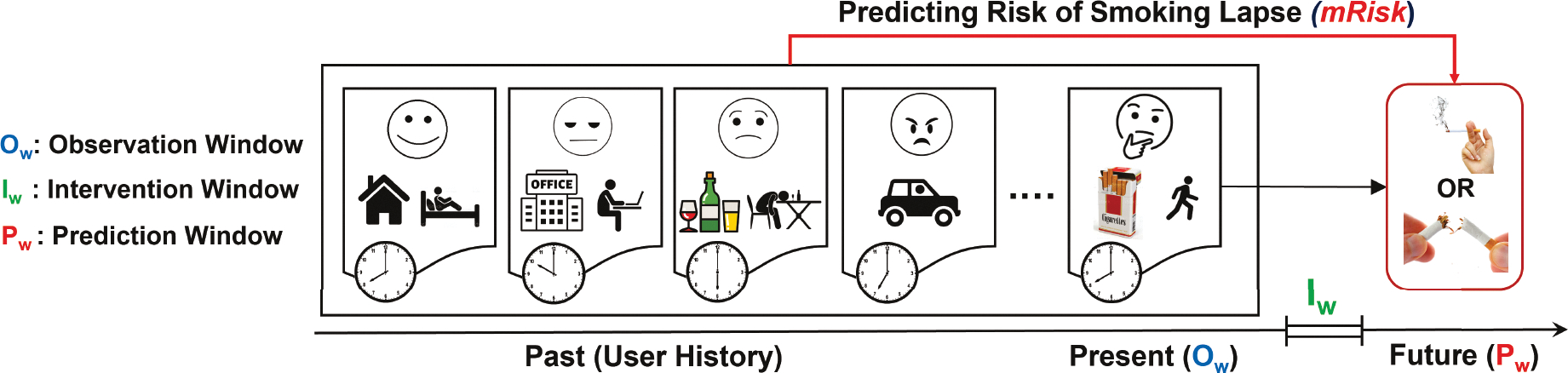
Internal state and external cues from an observation window and prior to it are used to estimate the risk of a smoking lapse during the prediction window. The intervention window between the observation and prediction windows gives an opportunity to deliver an intervention.

Problem:

Given the time series of sensor data and the timing of some smoking lapses from a population of abstinent smokers, train a model $ℳ$ that can accurately estimate the risk of lapse in a prediction window P_w for an abstinent smoker, using the sensor data observed up to and including the corresponding observation window O_w, such that the proportion of all prediction windows estimated to have a high-risk of lapse is minimized.

4. ROBUST COMPUTATION OF PSYCHOLOGICAL, BEHAVIORAL & ENVIRONMENTAL CONTEXT

We apply existing trained models to accelerometry, ECG, Respiration, and GPS data to capture the following psychological, behavioral, and environmental contexts of users, as continuous inference streams (see Figure 2a).

Fig. 2.

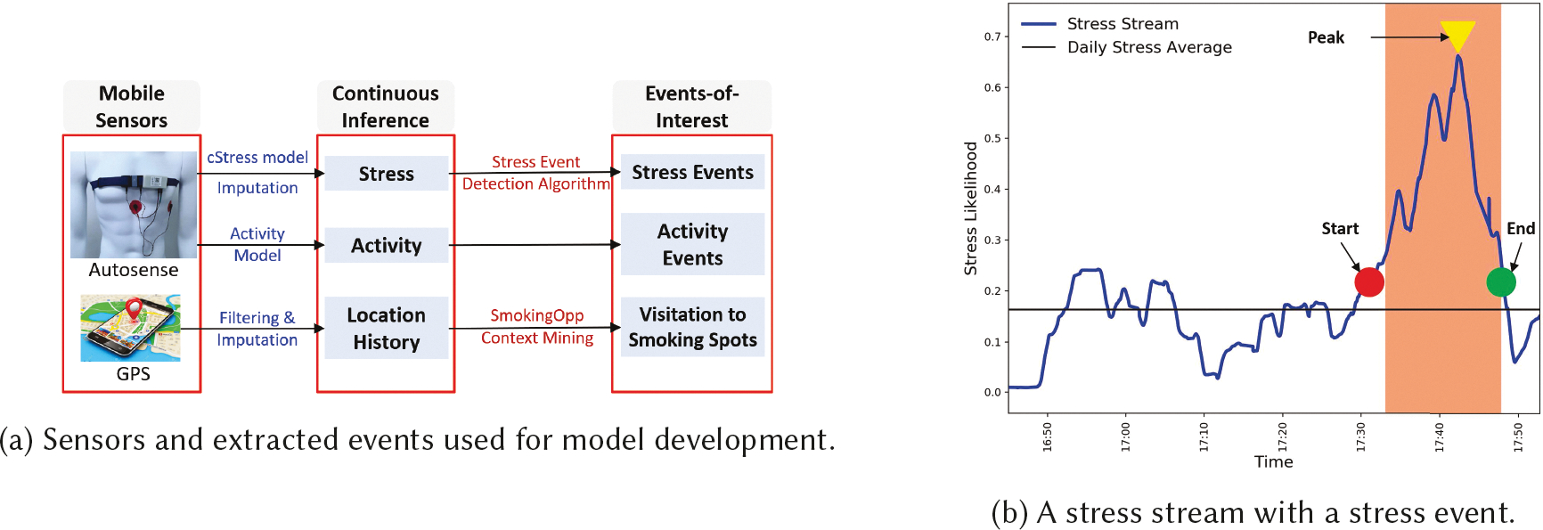
(a) Sensors and extracted events used for model development. (b) A stress stream with a stress event

Stress:

As stress can influence a smoking lapse, we obtain a continuous assessment of physiological stress arousal by applying the cStress model [27]. cStress computes a set of features from one-minute windows of ECG and respiration data and produces a likelihood that the user is exhibiting stress arousal in the captured physiological response. We apply the cStress model on our smoking cessation field study ECG and respiration data to generate stress likelihood every five seconds from overlapping, i.e., sliding minute windows to get a smoother time series. The cStress model produces a value between 0 and 1 that we call our stress inference stream.

We handle short episodes of missing data in the stress inference stream (due to noisy data, confounding physical activity, or recovery from physical activity), by applying the k-nearest neighbor-based imputation [60].

Activity:

Movement such as transition from inside to outside of a building can expose a user to potential environmental triggers of a smoking lapse (e.g., corner of a building designated as a smoking spot). Therefore, we obtain an assessment of non-stationary or active state for each minute. We utilize the 3-axis accelerometer sensor embedded in AutoSense for activity detection (of the torso) using the model presented in [52].

Location History:

Change in location can expose a user to major environmental cues such as tobacco point of sale or bars. Therefore, we obtain a continuous assessment of change in a participant’s location. We adapt the context mining approaches used in [9] to derive location history, dwell places, and transitions from raw GPS data. First, we de-noise the GPS data via median filtering [83] as the gap between consecutive GPS points is much less than fifty meters even at a speed of 100 kilometers per hour due to the sampling rate of 1 Hz in our GPS data. We perform median filtering by substituting a GPS sample point with the median of temporal predecessor points from a window length of 2 minutes (i.e., 120 predecessor points). This step produces a continuous inference stream of location history (time, latitude, and longitude). Finally, we employ spatio-temporal clustering to derive the start and end times at dwell places (both significant and transient) or transition from one place to another.

4.1. Robust Representation of the Current Context

The current context, i.e., measures of stress, activity, and location history inferred from the observation window, are heterogeneous as they are sampled at different rates, and transitions can happen dynamically. Although not as noisy as the raw sensor data they are derived from, they still suffer from noise, discontinuity, and rapid variability due to model imperfections, sensor non-wear, data quality issues, and confounding events.

To address these issues and obtain a homogeneous and robust representation of the current context that can be used to train a deep learning model, we compute statistical features of continuous inference streams. Such aggregate statistical measures have more robustness to noise compared to raw inferences themselves.

We use 13 statistical functions to compute features from the stress stream. These functions compute the elevation (80^th, 90^th, and 95^th percentiles), reduction (20^th, 10^th, and 5^th percentiles), dispersion (interquartile_range and skewness), central tendency (median), shrinkage (range between [20^th, 10^th] and [20^th, 5^th] percentiles), or accumulation (range between [80^th, 90^th] and [80^th, 95^th] percentiles) from a window of inferences. Given an observation window (t_i, t_i+w) of length w = |O_w| minutes, we have a maximum of 12 * w stress state data points, since an assessment is produced every 5 seconds. We compute stress features as follows. Thirteen (13) statistical features are obtained from the stress stream from t_i to t_i+w. The same functions are also applied to the consecutive difference between the successive stress likelihoods in the window. To account for day-specific within-person variability, we compute the statistical features (called baseline features) from day-long stress stream up to t_i+w (we use until_obs to abbreviate ‘until the end of observation window’). Finally, we capture the average deviation of stress (from the daily mean) at the current window.

We compute the fraction of time active in the current window from the activity stream in an observation window. From the location stream in the observation window, we compute a binary indicator to check if the current location is a smoking spot (=1) or not (=0). Next, we compute the distance to the nearest smoking spot. Finally, we compute the fraction of time spent stationary at a place, the fraction of time spent in transition in the current window and the current speed.

In total, we compute 46 features from the three inference streams, called the Continuous Inference Features.

4.2. Encapsulating History via Events-of-Influence

A key question for the mRisk model is how to describe the influence of context on lapse risk over time. Continuous measures of factors such as stress are likely to have only proximal impact on risk, which is modeled by the temporal interval between the observation and prediction windows. However, significant contextual events, such as period of extremely high stress, may have a degree of influence over a significantly longer interval of time. We, therefore, define events of influence, which are specific contextual events occurring at discrete moments in time, and model their influence on risk prediction. Hence, our next challenge is how to succinctly capture the influence of these historical contexts so that the model may be able to estimate the degree of their influence and how it may wane over time. We encapsulate the historical contexts by computing events-of-influence streams (see Figure 2a) from the corresponding continuous inference streams.

Event-of-influence stream is a sequence of irregularly spaced events derived from the continuous inference stream. An event represents a location in time, which likely impacts the participant’s current and future actions. Each event comprises of one or more attribute values, a start time, and an end time, represented as <list of values, start, end>. The type of attribute values in different events-of-influence stream can be numerical, binary, or categorical. Specifically, we compute three events-of-influence streams.

4.2.1. Stress Events.

The model presented in [60] applies a moving average convergence divergence (MACD) method to detect the increasing or decreasing trend and the inflection point (or the peak) in the stress likelihood time series based on short-term and long-term exponential moving average. This method clearly marks each stress event’s start and end times, defined as the interval containing the increasing-trend interval followed by a decreasing-trend interval. Each stress event has the following attributes — the stress duration, which is defined as the time interval between the start and end of a stress event (in Figure 2b, we observe a stress event of 14.75 minutes) and the stress density, which is defined as the area under the stress stream divided by the stress duration (in Figure 2b, we observe a stress event with density of 0.445). Each stress event is represented by <stress density, stress duration, start, end>. Finally, the model applies a threshold based on the stress density to determine which events are stressful and which are not. We note that stress or non-stress events are only detected from those segments of sensor data that are of acceptable quality and not confounded. In our data, on average, we detect 2 to 9 stressful events per day with a mean density of 0.242 and a mean duration of 10.747 minutes.

4.2.2. Activity Events.

We employ the following approach to detect the activity events from the activity stream. We cluster the contiguous active and stationary windows together to construct the active and stationary events, respectively. Each activity event is represented as <binary indicator of 1, duration, start, end>. In our data, on average, we detect 12 activity events per day with a mean duration of 2.70 minutes.

4.2.3. Visitations to Smoking Spots.

Smoking spots are those places where participants are observed to have smoked, smoking is usually allowed, and cigarettes are available. We employ the spatio-temporal context mining methods described in [9] to locate the two categories of smoking spots (personal and general smoking spots) from participant’s location history and smoking patterns.

Visitations to smoking spots are recorded as events-of-influence. We adapt the method from [9] to detect a visitation to a smoking spot (when a participant dwells for at least 6.565 minutes with the distance of 30𝑚 from the centroid of a smoking spot). Each visitation to smoking spot event is represented as <semantic type, duration of stay, start, end>, where we consider the following semantic types for our analysis, smoking outlet, retail store, gas station, or a bar (usually cigarettes are available at these location types), start is the arrival time to and end is the departure time from the smoking spot. Duration of stay at a smoking spot is computed as the difference between the departure and the arrival time. In our data, on average, we detect about 1 visitation to smoking spots per day with a mean stay duration of 12.48 minutes.

5. mRisk: MODELING IMMINENT RISK OF LAPSE

In developing the mRisk model, we aim to discover a suitable representation of the event-of-influence time-series and find the role of continuous context variables within the observation window in predicting the lapse risk. We first opt for traditional feature representation of the event time-series. We propose several features to summarize the influence of events on modeling the lapse risk phenomenon. We term this model Deep Model with Recent Event Summarization (DRES). In an alternate approach, we hypothesize that events have a decaying influence over time on the risk of lapse. We explicitly model the decaying influence using exponential decay functions. Furthermore, we incorporate knowledge from the patient sub-typing domain [3] to enable end-to-end model learning, with both dynamically changing instance variables and static variables reflecting an aggregate phenomenon. We refer to this model as Deep Model with Decaying Historical Influence (DDHI).

5.1. Deep Model with Recent Event Summarization (DRES)

For the DRES model, we represent the event-of-influence Using features. These features complement the statistical features obtained from the observation window described in Section 4.1. The architecture of the DRES model also includes the encoding of the recent past with a stacked observation window-based design. We present the features used to summarize the events-of-influence and the model architecture in the following.

5.1.1. Events-of-Influence Representation using Features.

We propose 15 events-of-influence features to capture the temporal dynamics of the psychological, behavioral, and environmental events from the recent past. These features are extracted from three events-of-influence streams corresponding to an observation window.

• Stress Events: We compute average duration & density of stress events within current window, time since the previous stress event, duration & density of the previous stress event. Additionally, we compute the average duration & density of stress events, and fraction of time in the stressed state until the observation window.

• Activity Events: We compute time since the previous activity event and duration of the previous activity event. Additionally, we compute the average duration of activity events and fraction of time in an active state until the observation window.

• Visits to Smoking Spot Events: We compute time since last visit to a smoking spot and average duration of stay at smoking spots. We also compute the fraction of time spent at smoking spots until the observation window.

5.1.2. Feature Set.

We compute 61 total features from the continuous inference and event-of-influence streams. We also include the hour of day (using one-hot encoding) as a feature based on prior work [64] which shows time may affect the occurrence of a smoking lapse. In total, we compute 62 features per observation window for the DRES model development. We adopt per-participant standardization to account for between-person differences and introduce feature baselines to incorporate within-person variability or individual biases in features.

5.1.3. DRES Model Architecture.

The idea behind the DRES model is that all the features computed in each observation window can be represented in a time-lagged fashion to accurately estimate the risk of lapse likelihood in the prediction window. Figure 3 shows the overall architecture of DRES model. Here, X_t refers to the feature vector computed from an observation (i.e., time-lagged) window starting at time t. We use the tabular features n_f = 62 from each observation window. Next, we stack features from n_l previous observation windows, with the size of the input instance being n_l × n_f. The n_l observations provide information on the temporal evolution of features in the recent past (hence, the term Recent in DRES). The efficacy of DRES model depends on the ability of hand-crafted features to properly encapsulate the spatial-temporal-behavioral cues useful in predicting lapse. Since DRES model utilizes regularly sampled feature vectors stacked together in time, we use a simple Convolution plus LSTM architecture. The model’s overall architecture consists of two convolutional layers, one recurrent LSTM layer, three fully connected layers, and a single node sigmoid layer. The convolution layers help to extract micro-features in a local neighborhood followed by an LSTM layer which captures temporal patterns of the micro-feature sequence. The recurrence in the LSTM is operating along the n_l lagged windows. The penultimate fully connected layer is followed by an L₂ normalization layer to normalize the input vectors to unit norm. Finally, the output of the final fully connected layer is passed through a single node with a sigmoid activation function to generate the lapse likelihood.

Fig. 3.

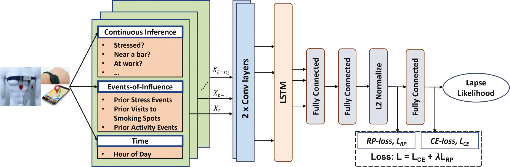
Overall architecture of the Deep Model with Recent Event Summarization (DRES).

5.2. Deep Model with Decaying Historical Influence (DDHI)

For the DDHI model, we explicitly model the decaying influence of a past event. For the current context, we continue to use the statistical features from Section 4.1. But, we observe that the proposed event of influence features in the DRES model rely heavily on the usefulness of specific features calculated and are limited to only incorporating the most recent past events and the average information. We propose an alternative event encoding approach that allows for encoding of multiple past events and enables the model to learn from not only recent events but also the accumulated effect of past on participants’ psychological and contextual state without explicit feature engineering. First, we provide the rationale for the development of our proposed methodology. Next, we formally define the encoding procedure and the various design choices involving the model architecture.

5.2.1. Modeling Rationale.

Lapse risk may be influenced by not only recent internal and external events but also by the accumulated history of exposures, with the influence waning over time. To model this behavioral element, we need to efficiently represent the stimuli received by the participants from earlier time points. In estimating the risk of imminent adversarial behavior, our goal is to directly account for the current influence of past events, weighted by their position in time. The event-of-influence streams are also unique in their discrete nature of non-aligned multi-modal observation. The unique aspects of event modeling make it challenging to directly apply the current deep-learning modeling approaches to our scenario.

Modeling with time-series data requires encoding previous states as time progresses. Long-Short Term Memory Networks (LSTMs), Time-Aware LSTM networks [3], and attention-based LSTMs [78] have all been used successfully to model time series data. They have produced state-of-the-art results in time-series problems such as mood forecasting [70], mortality prediction [10], and intervention delivery [72]. Transformers [77] with the self-attention mechanism has proven highly successful in modeling long-term dependencies for sequential data, enabling learning of large sequence models for multivariate long-term forecasting [84].

In our case, to capture the historical influence, the model needs to learn from the events-of-influence streams. Different events-of-influence streams have observations at different times with scant alignment between them. To properly capture the historical influence, we need to be able to learn from these multiple irregular time series from further in the past. We also need the model to learn from mutual interaction of multiple past event types by aligning their decaying effect in a future time, which is not yet handled well in current models. To efficiently model long-range temporal interactions of irregularly sampled non-aligned observations, we want a model where the temporal delay can be explicitly designed because it’s a key aspect of our problem.

Therefore, we propose a decay-aware temporal embedding of heterogeneous past events to encode their residual effects in predicting the lapse risk. We represent each event using a standard set of attributes and use the encoding approach to propagate the effects of past events. In this way, we aim to create a temporal projection of any past event in times of future inference. Our proposed methodology transforms event data using an exponential decay function before feeding it to an LSTM layer. The LSTM layer provides a simple way of handling the time-dependency within the current observation of limited length. To estimate effective exponential decay factors and weights for different event attributes, we adopt the patient phenotyping approach from the EHR domain [3]. We analyze the feasibility of grouping our participants using global aggregate context variables from the pre-quit period and use the grouped representation as a key input variable in the model.

5.2.2. Decay-aware Temporal Encoding of Heterogeneous Events.

We represent a single event using a vector of k attributes, B = [β₁, β₂, ..., β_k] alongside the time of event t. For example, stress events can be represented using, the time of event t, density β₁, duration β₂, peak amplitude β₃ and other factors. These attributes are determined by the event type. For example visit to smoking spots is an indicator event with no density information present. We represent a single event of type e (e.g., stress, visit to smoking spots, activity) using the tuple $\left(t,B^e=\left[{\beta }_1^e,{\beta }_2^e,\dots ,{\beta }_k^e\right]\right)$. We aggregate the contributions of k different attributes of an event in a single numerical value using a linear function,

$$f\left(B^e\right)=\frac{1}{k}\sum _{i=1}^k{\mu }_i^e{\beta }_i^e$$ (1)

Here, ${\mu }_i^e$ is the weight coefficient associated with the i^th attribute,${\beta }_i^e$. We standardize each attribute to be within the range [0, 1] and estimate the weight coefficients using sigmoid function —$0\le {\mu }_i^e\le 1$. The division by the number of attributes k ensure that 0 ≤ f(B^e) ≤ 1 for all event types with different number of attributes.

To represent an event from the past (t₁, B^e) at a future time t ≥ t₁, we assume an exponential decay function of a constant rate α^e with f(B^e) representing the initial quantity from (1). Thus, the contribution of the event from time t₁ at a future time t becomes $f\left(B^e\right)e^{-{\alpha }^e\left(t-t_1\right)}$. Exponential models are widely used to model decay in natural phenomenon such as drug absorption [25], recovery times from physical activity [60], among others.

Thus, given n past events of Type e, $\left(t_1,B_1^e\right)$, $\left(t_2,B_2^e\right)$, $\left(t_3,B_3^e\right),\dots ,\left(t_n,B_n^e\right)$, we aggregate the effects of all past events at time t as ${\widehat{s}}_t^e$ with

$${\widehat{s}}_t^e=\sum _{k=1}^{n}f\left(B_k^e\right)e^{-{\alpha }^e\left(t-t_k\right)}I\left(t\ge t_k\right),$$ (2)

where I (t ≥ t_k) is an indicator function equal to 1 if t ≥ t_k and 0, otherwise. The parameter α^e controls the rate of decay of an event of type e as we progress in time. We directly feed the time-series ${\widehat{S}}_{t-w:t}^e$ of different event types (stress, activity, smoking spot visits) to the model together with statistical features from the current window O_w to allow the model to learn from accumulation of past events. Since Equation 2 can be computed at any time in future, we can maintain the regular time intervals required for a simple LSTM to operate on.

Our embedding depends on effective estimation of the parameters α, [μ₁, μ₁, ..., μ_k] for each event type. We assume that these three parameters act as variables specific to global contexts. For example, we assume that the decaying rate of influence of stress on lapse risk does not change from one stress event to another and is similar for a set of homogeneous participants (i.e., phenotype). Thus, estimation of the parameters α, [μ₁, μ₁, ..., μ_k] depends on identifying the degrees of freedom on which each participant is homogeneous.

5.2.3. Phenotyping Participants for Parameter Estimation.

Patient sub-typing is grouping of patients to address the heterogeneity in the patients, to enable precision medicine where patients are provided with treatments tailored to their broadly unique characteristics [3]. We group participants based on observations from the pre-quit period so that the model can be applied to a user right from the moment they quit when no post-quit data is available. The features we use include gender, age, average stress density, duration and count per day before quitting, average frequency and duration of visits to smoking spots prior to the quit period, and average activity event count and duration per day. We term them phenotype features since they provide relatively stable information (i.e., trait) about the participants. We aim to cluster the participants into a small number of groups.

Clustering:

Our clustering of participants based on their phenotype features is guided by three questions — which clustering algorithm to use, which features contribute most towards a grouping of the participants, and how many clusters are appropriate. We experiment with partition-based traditional k-means algorithm and hierarchical clustering approaches. Both methods perform similarly in our data. We vary the number of clusters for obtaining the most appropriate clustering. For identifying the features which are most useful in grouping the participants into different clusters, we select silhouette score [54] as the evaluation criterion. First, we re-scale the features to fall within the same range between 0 and 1. Next, we measure the silhouette score of removing a single feature at every iteration and remove the feature which contributes negatively toward the overall clustering. This recursive feature elimination process allows for identification of the most important features necessary for grouping the participants. Finally, we apply the k-means clustering with appropriate number of clusters for extracting groups of similar participants. Using number of clusters equal to 4, we obtain the best result with all the features contributing positively. The centroid of each cluster is used to estimate the parameters α, [μ₁, μ₁, ..., μ_k].

5.2.4. DDHI Model Architecture.

Figure 4 shows the overall architecture of the end to end DDHI model. The phenotype features are first used for clustering the participants. The mean of each cluster is then used to output three global context specific parameters (α, μ₁, μ₂) for each event type using a feed forward layer. The centroid of each cluster represents all the participants belonging to that cluster. The centroid is passed as an input through an intermediate feed forward layer. α, [μ₁, μ₁, ..., μ_k] are weights of nodes with sigmoid activation function which are fully connected to the mentioned intermediate layer. Using the appropriate parameters for each event type, the event log in the memory are then transformed to form the event encoded time-series ${\widehat{S}}^{stress}$, ${\widehat{S}}^{activity}$, and ${\widehat{S}}^{smk\_spot}$. Let the length of the current observation window be equal to w with rightmost time t. Then, we output the event of influence encoded time-series for r separate event types within the current observation window as ${\widehat{S}}_{t-w:t}^{even{t}_{1}even{t}_2,\dots ,even{t}_r}\in {ℛ}^{w\times r}$, where ${\widehat{s}}_{t-w:t}^{stress}$ measures the aggregate effect of all past stress events in the current time window t − w to t. The features from continuous inference streams along with the hour of day are used in a lagged fashion with multiple observations of n_f = 47 features. With n_l such lags, a single instance of lagged features is $X_{t-n_l:t}\in {ℛ}^{n_l\times n_f}$. Two separate LSTM networks are trained on top of the lagged features $X_{t-n_l:t}$ and ${\widehat{S}}_{t-w:t}^{stress,activity,\mathrm{...},smk\text{\_}spot}$. We flatten the outputs of LSTM into planar nodes, concatenate the two separate representations and feed it to a multi-layer feed-forward neural network.

Fig. 4.

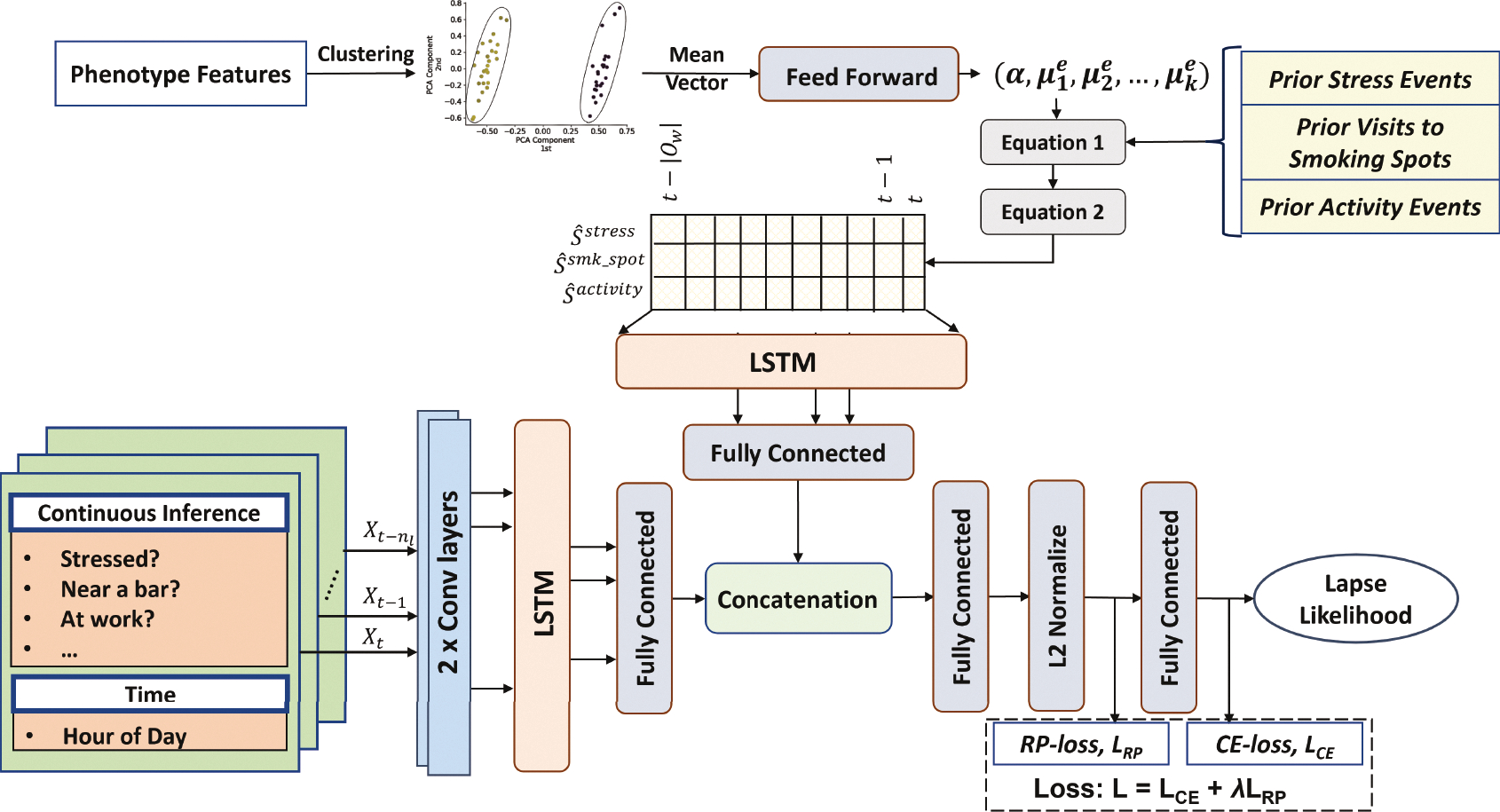
Architecture of the Deep Model with Decaying Historical Influence (DDHI) that uses an explicit model of decaying influence of past events that are expected to wane over time.

6. LEARNING FROM SPARSE & POSITIVE ONLY LABELS

Our goal is to estimate the risk of a smoking lapse during the abstinence period from continuous sensor data in the natural environment. We segment the sensor streams using sliding (by 1 minute) candidate windows consisting of the observation, intervention, and prediction windows. We assign a positive-label (high-risk of lapse) to observation windows only if the corresponding prediction windows overlap with a smoking lapse time, otherwise, the observation windows are unlabeled. Recall that we only consider a lapse to have occurred if it is detected by puffMarker and supported by an EMA. Using either of them alone is insufficient since self-report does not pinpoint the accurate timing of smoking lapse, and puffMarker can produce false positives. As a consequence, our available ground truth labels are sparse, and we only have positive (high-risk) labels available.

6.1. Positive Unlabeled (PU) Learning

As we only have access to a subset of positively-labeled data and a larger class of unlabeled data which may consist of many lapse events that were either missed by puffMarker, missed by EMA, or missed by both, we adapt positive-unlabeled (abbreviated as PU) learning methods to train the mRisk model choices. PU learning [4] is a variant of the classical supervised learning setup where the assumption is that the data contains positive-labeled or unlabeled samples, which may contain positive (high-risk of lapse) or negative (low-risk of lapse) samples. We employ class-weighted base estimators in the PU learning framework to address the class imbalance.

As we mark an observation window with a positive label if the corresponding prediction window overlaps with the smoking lapse time, the traditional assumption that positively-labeled data is selected completely at random (SCAR)) does not hold. Therefore, we use the PU-bagging or ensemble PU learning approach [46] that is independent of the SCAR assumption and use leave-one-participant-out-cross-validation (LOPOCV). We describe more details of how we train the PU-bagging model in the Appendix (see Section A.1).

6.2. Rare-Positive (RP) Loss Function

Key to training deep learning models is a suitable loss function that the model can use to optimize the representation. Contrary to the typical supervised learning setup, where concrete ground truths are available for both positive and negative classes, we only have access to a subset labeled positives (i.e., high-risk moments). All the other samples are unlabeled and consist of positives (i.e., lapses missed by puffMarker and/or EMA) and negatives (low-risk moments); we assume that the proportion of positive instances is rare in the unlabeled class. We want to guide the learning process so that the model learns an accurate representation of the positive class and learns to extract other rare true positives from the unlabeled class.

6.2.1. Design of the RP Loss Function.

In designing the RP loss function, we aim to achieve two key goals. First, we want to create a representational feature space in which positive data points are clustered together. This is trivial for the model to do by coalescing all the input instances into a single point in the feature space. Hence, the second condition needs to be designed, which constraints such development. Our second competing goal is to ensure that the learned representation space of the positive class can only include a small portion of the unlabeled class, as positive instances are expected to be a rare occurrence in the unlabeled class. To formulate the two components of our proposed loss function, we let $\mathbb{S}$ denote the set of all samples, ${\mathbb{S}}_p$ the set of all positively-labeled samples s_p and ${\mathbb{S}}_u$ the set of all unlabeled samples s_u, with $\mathbb{S}={\mathbb{S}}_p\cup {\mathbb{S}}_u$.

Positive Class Dispersion (P):

We adopt the definition of consistency as proposed recently in [56], to minimize intra-class variations, but apply it only to the positive class $\left({\mathbb{S}}_p\right)$. Our goal is to reduce the mutual dispersion of the positive instances for forming dense clusters. As in [56], our data is also collected by wearables in the noisy field environment, and hence are impacted by outliers. To reduce the impact of outliers, we also define dispersion of the positive class $\left({\mathbb{S}}_p\right)$ in terms of a robust aggregate function.

Consistency of $s_p^i\in {\mathbb{S}}_p$ is the average distance of its representation from the representation of all other points $s_p^j\in {\mathbb{S}}_p$, i ≠ j in the model’s feature space, i.e., $C\left(s_p^i\right)=d\left(s_p^i,{\mathbb{S}}_p\right)$, using the definition of average distance in the feature space from [56]. It was shown in [56] that this definition of distance is differentiable and hence suitable for use in loss function and leads to faster convergence (for noisy data collected by wearable devices). Now, consistency of the positive class is defined as an aggregated function, ψ, of all the point consistencies within the class. Within a mini-batch of data ${\mathbb{U}}_{MB}\in \mathbb{S}$, positive class dispersion, P is defined as

$$P=\psi \left({\left\{C\left(s_p^i\right)\right\}}_{s_p^i\in {\mathbb{U}}_{MB}\cap {\mathbb{S}}_p}\right)$$ (3)

Similar to [56], we also select a percentile measure for ψ. But, in contrast with [56] that uses non-overlapping windows of data, we need to produce a risk score for each minute and hence use overlapping windows, sliding each minute. Consequently a positive event (i.e., a confirmed lapse) is contained in all overlapping observation windows whose prediction window (e.g., 60 minutes long) contains the positive event. One positive event a day can result in 10% (60 out of 600 minutes of sensor wearing a day) of the data labeled as high-risk. Therefore, we use 80^th percentile of the point consistency values of the positive class to obtain robustness, while respecting rarity of the positive class. Minimizing P ensures that the positive instances pack tightly in the deep representations space.

Rarity of the Unknown Positives Within Unlabeled Class (R):

Given the assumption of rarity of positive samples in the unlabeled class, the tight cluster produced for the positive class (by minimizing P) should only contain a small portion of the unlabeled class. For this purpose, we define the rarity metric R as the proportion of unlabeled samples whose average distance from the samples of positive class are at most P.

Let $d\left(s_u^i,{\mathbb{S}}_p\right)$ denote the average distance of the representation of unlabeled sample $s_u^i\in {\mathbb{S}}_u$ from the representation of all positive instances $s_p^j\in {\mathbb{S}}_p$ in the model’s feature space. We define an indicator function

$$I\left(s_u^i\right)=\{\begin{array}{ll}1\hfill & d\left(s_u^i,{\mathbb{S}}_p\right))\le P\hfill \\ 0\hfill & \text{otherwise}.\hfill \end{array}$$

Our goal is to limit the number of unlabeled instances for whom the above indicator function outputs 1. For this purpose, given a mini-batch of data instances ${\mathbb{U}}_{MB}\in \mathbb{S}$, we define the rarity metric R as follows.

$$R=\frac{{\sum }_{s_u^i\in {\mathbb{U}}_{MB}}I\left(s_u^i\right)}{\left|{\mathbb{U}}_{MB}\cap {\mathbb{S}}_u\right|}$$ (4)

Minimizing R amounts to reducing the proportion of unlabeled instances which fall within the cluster of positive instances and minimizing P constraints the positive instances to form a tight cluster itself.

We compose our overall Rare-Positive (RP) loss function as follows so the model can concurrently optimize both positive dispersion (P) and rarity (R) measures.

$${ℒ}_{RP}=\gamma P+{(R-ϵ)}^2,$$ (5)

where ϵ is the expected proportion of unknown positives we assume to be present within the unlabeled class. (R − ϵ)² denotes the squared distance of the rarity metric R from a fixed ϵ value. We choose the quadratic function in favor of an absolute error for two reasons. First, quadratic error term is continuously differentiable. Second, we want the penalty for an error to increase in proportion to the magnitude of the error itself.

We conduct experiments to find the best value of ϵ from our dataset. The γ value is a scaling hyper-parameter for scaling two terms with different units. Since, we L₂ normalize the deep vectors to have unit norms before distance calculation, their range is similar to the range of proportions (0, 1). We choose γ = 0.5 for our experiments.

6.2.2. The Loss Function.

For training the mRisk model, we employ the joint supervision of cross-entropy loss (to derive risk likelihood between 0 and 1) and RP loss. More specifically, our overall loss objective is

$$ℒ={ℒ}_{CE}+\lambda {ℒ}_{RP},$$ (6)

where ${ℒ}_{CE}$ is cross-entropy soft-max loss [81] and we use λ (= 0.2) to balance the effect of two loss functions.

7. OPTIMIZATION, EVALUATION, AND EXPLANATIONS OF mRisk MODEL CHOICES

We first determine the best value of the hyper-parameter ϵ to optimize the proposed RP loss function. Second, we compare the performance of our two proposed models by analyzing the risk characteristics each model produces. Third, we design simulation experiments to evaluate how successful the models are in creating intervention opportunities prior to each confirmed lapse. Fourth, we visually analyze the risk dynamics produced by mRisk before and after lapse moments. Finally, to understand the major factors driving the lapse risk produced by the mRisk model, we explain the influence of features on the model performance using Shapley values [42].

7.1. Loss Function Optimization and Evaluation

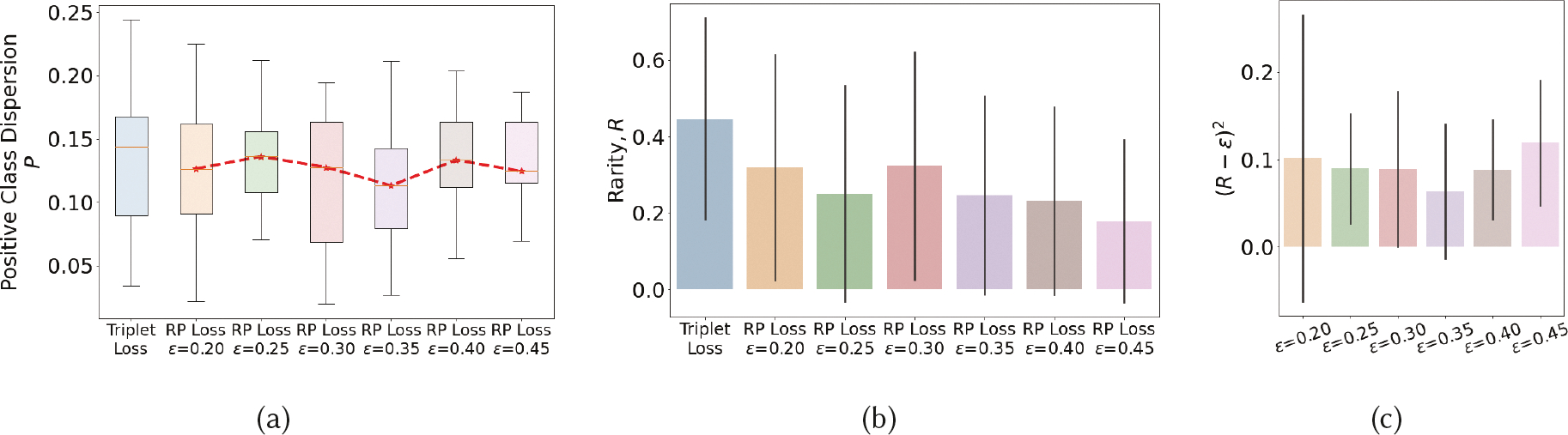
We experiment with different choices of ϵ (which denotes the expected proportion of rare positives within the unlabeled class) on positive class dispersion (P) and rarity metric (R) to determine its best value. We also compare with Triplet loss [61], a widely used traditional loss function used in deep learning. Figure 5 shows the results when we train the models by combining the stated loss functions with cross-entropy loss. We make several observations. As each model is trained with mini-batches, we first analyze the distribution of P and R for different choices of ϵ. We observe that the model achieves lowest deviations (or spread) in P and (R − ϵ)² for ϵ = 0.35. We take this as an indication that for this value of ϵ, the model is able to consistently find the best representation to separate out positives (including unknown positives in the unlabeled class) from the negatives (all in the unlabeled class). We get another supporting indication of it by observing that the value of P is the lowest for this choice of ϵ. We see from Figure 5c that when ϵ increases from 0.2 to 0.35, the weight assigned to the (R − ϵ)² component of the RP loss function reduces because 0 ≤ (R − ϵ) ≤ 1. After this value, ϵ gets farther away from the true proportion of positives in the unlabeled class (see Figure 5b), making it harder for the model to find a suitable representation. Therefore, we hypothesize that for ϵ = 0.35, the model is able to find a representation to form the tightest cluster of positives while allowing unlabeled positives. We use ϵ = 0.35 for all experiments.

Fig. 5.

P and R values when using different values of ϵ in the RP loss function, compared with that from using Triplet loss.

We next observe from Figure 5b that at ϵ = 0.35, the proportion of unlabeled positives is 24.68% of the unlabeled data (i.e., R). We use EMA reported lapses that were not used in model training (as they were missed by puffMarker) to estimate the proportion of positive class in unlabeled data. Each EMA where one or more lapses was reported, indicates a 2-hour lapse window where participants recall having smoked. If these hours are considered to represent high-risk moments, they constitute 17.8% of all unlabeled hours of data. As the high-risk moment is considered to precede a smoking lapse, the entire 2-hour window may not constitute high-risk moments, while hours where no lapse was reported may also consist of high-risk moments, this is only a crude estimate based on available sources of imprecise labels. Nevertheless, the two estimates lie within 7% of each other.

We also observe that treating the unlabeled data as negatively labeled and using Triplet loss to maximize its separation from the positive class results in a representation that produces slightly higher values of P as the RP loss function (especially for ϵ = 0.35). But, as the model is forced to maximally separate positives from the unlabeled class, it ends up admitting a larger proportion of unlabeled data (about 45%) in the positive cluster. Using a model trained with such a loss function will require a higher number of interventions to achieve a given recall rate (i.e., intervention delivered prior to a detected lapse event) as compared with the RP loss function.

7.2. Evaluating mRisk Model Choices by Their Risk Characteristics

We train the two mRisk model alternatives using only sparse positive labels. Lack of unambiguous negative labels of low-risk moments diminishes our options of computing traditional metrics such as F1 score, AUROC, and others. Thus, we opt for measuring the performance of the models in predicting the detected lapse events. If the model outputs a high-risk probability for a confirmed smoking lapse, we consider it an accurate prediction.

However, if we classify every data-point as high-risk, we would achieve 100% accuracy. In a traditional supervised learning setup, we measure the false positives, which gives us a measure of the cost of using/deploying any developed model. Since we can not measure the false positive rate directly, we propose to measure the cost of our model indirectly. At every decision point, we treat the percentage of assessment windows determined to be high-risk as the cost of a specific model. This indirectly captures the user burden posed by a model in real-life where a high-risk moment may trigger an intervention to reduce the likelihood of a lapse.

We also note that considering any data-point as high-risk requires specifying a decision threshold (T_L) within the probability scale. If the model outputs a probability ≥ T_L, we consider it a high-risk moment, and low-risk, otherwise. We select a value of T_L to achieve a lapse detection accuracy of 80% and report the inference cost.

7.2.1. Results.

Figures 6a and 6b together captures the trade-off between lapse detection performance and the inference cost for using different values of the decision threshold (T_L). Figure 6a shows the steep drop-off in detection accuracy for both the mRisk model choices as we increase the value of the decision threshold. The drop-off in accuracy is comparatively less steep for the DDHI model when compared to the DRES. For achieving a minimum of 80% lapse detection performance, the decision threshold values are 0.28 for the DRES model and 0.31 for DDHI. The corresponding inference costs are 33.61% and 24.50% for DRES and DDHI respectively. Thus, for the same lapse detection performance, we obtain a 9% improvement in the inference cost by using the DDHI model. Figure 6c shows the distribution of the lapse likelihoods produced by both models. Both models have the desirable right-skewed distribution, as we expect a majority of moments to represent a low risk.

Fig. 6.

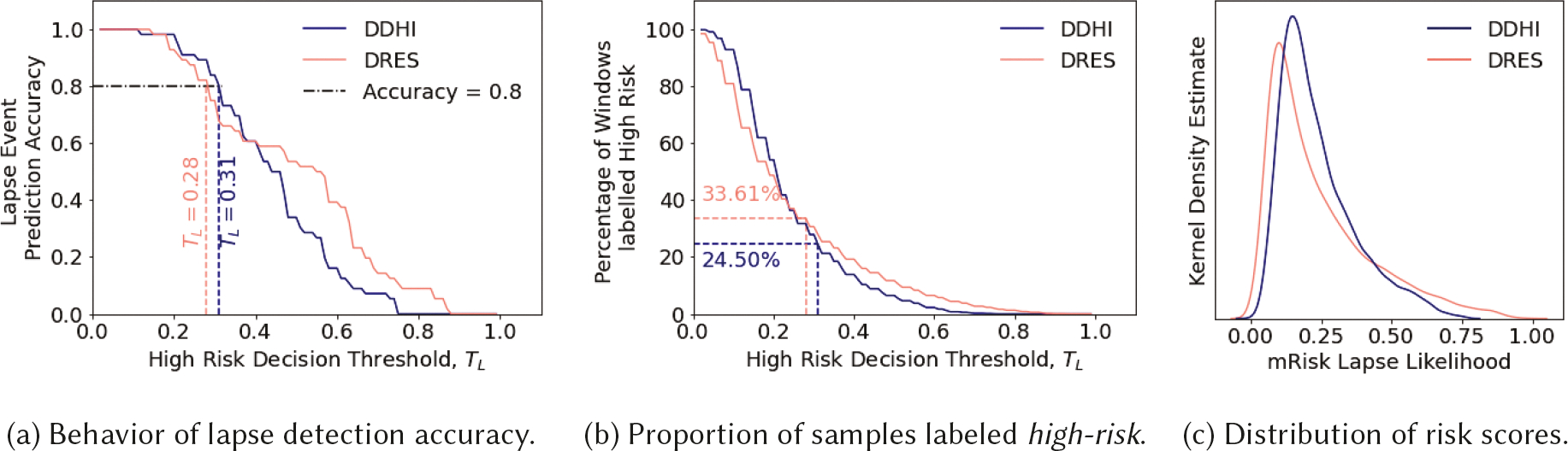
Evaluating mRisk model choices on PU-labeled data.

7.3. Evaluating mRisk Model Choices via Simulated Delivery of Risk-Triggered Interventions

For our next evaluation of the two models, we train a baseline machine learning model and evaluate how successful the models are in creating intervention opportunities prior to each confirmed lapse. We design simple simulation experiment where interventions are delivered when the risk for lapse rises above a pre-determined threshold (T_L) (see Section 7.2). To limit intervention fatigue [32], no new interventions are triggered until intervention gap (I_G) minutes have elapsed since the last intervention, assuming the impact of an intervention lasts at least this long.

Since we use a prediction window of 60 minutes, we use I_G = 60 minutes. We note that introducing an intervention gap changes the direct relationship between the risk threshold and the frequency of interventions observed in Section 7.2. Although the choice of T_L and I_G will depend on the characteristics of the dataset, preferences of the smoking intervention researcher, and other real-life constraints (e.g., no intervention when driving or when in meetings), we analyze the performance of the mRisk model choices in the simple scenario when the intervention delivery only depends on T_L and I_G to show its expected behavior. Keeping I_G set at 60 minutes, we vary T_L to observe the performance of each model at different frequency of interventions per day.

7.3.1. Evaluation Metric.

For each model, we estimate the probability that an intervention opportunity is available ahead of a lapse event. For this purpose, we use only the confirmed lapse moments, i.e., positive labels. The proportion of lapse events occurring within 60 minutes (i.e., prediction window) of an intervention is called the Intervention Hit Rate (IHR) (see Section A.2 in the Appendix for a more precise formulation). As launching an intervention at every allowable moment can trivially achieve a 100% IHR, but at the cost of a high intervention frequency, we measure the participant burden via intervention frequency and determine IHR for different values of intervention frequency per day. For a given intervention frequency, a better model should have a higher IHR.

7.3.2. Experiment Setup.

We simulate with an intervention frequency range of [3, 7] per waking day to evaluate mRisk model choices — DRES and DDHI — in creating intervention opportunities. We also train a Random Forest Model using the PU Bagging Framework, named PU-Bagging RF [7], to act as a baseline. This model accepts the feature vector used in the DRES model, and produces a risk score for each observation window.

To vary the intervention frequency per day for the PU-Bagging RF, DRES and DDHI models, we vary the risk thresholds. In addition to evaluating the performance of the three models on IHR, we also compare the difference in IHR when using the new RP loss function versus Triplet Loss in both mRisk model choices. To evaluate the impact of phenotyping idea in the DDHI model, we experiment with different number of phenotypes, including no phenotypes. Finally, as learning the personal smoking spots for each new user requires collecting and analyzing pre-quit data, we evaluate the gain in performance when this data is used in modeling.

7.3.3. Results.

Table 1 shows that DRES and DDHI outperform the baseline PU-Bagging RF model, DDHI outperforms IHR, and RP Loss outperforms Triplet Loss. The last row in Table 1 shows that not using personal smoking spots results in a substantial drop in performance of both models. Table 2 shows the effect of phenotyping in the DDHI model. We observe that increasing the number of phenotypes improves IHR, achieving a peak IHR for four (4) phenotypes suggesting it as the optimal for our dataset. As the DDHI model with RP Loss function outperforms other models, we select this as the mRisk model in subsequent experiments. We select 5.5 interventions per day, as it provides the largest jump in IHR. We also find that for this choice, the risk crosses the threshold approximately 32 minutes prior to the lapse moment, on average, providing half an hour window to intervene prior to a lapse.

Table 1.

Intervention Hit Rate at Different Frequencies of Intervention for Different Models

		IHR at Different Frequencies of Intervention
Model	Loss Function	3	3.5	4	4.5	5	5.5	6	7	Mean IHR
PU-Bagging RF	–	0.30	0.37	0.49	0.64	0.70	0.75	0.75	0.76	0.60
DRES	Triplet loss	0.44	0.51	0.57	0.68	0.74	0.78	0.84	0.93	0.69
DRES	RP loss	0.46	0.55	0.64	0.74	0.76	0.78	0.84	0.93	0.71
DDHI	Triplet Loss	0.51	0.59	0.65	0.71	0.73	0.80	0.85	0.86	0.71
DDHI	RP loss	0.50	0.62	0.68	0.74	0.76	0.85	0.89	0.93	0.74
DDHI Without Personal Smk. Spots	RP loss	0.47	0.51	0.55	0.60	0.66	0.75	0.80	0.91	0.66

Table 2.

Intervention Hit Rates obtained from DDHI model with different number of phenotypes.

	IHR at Different Frequencies of Intervention
No. of Phenotypes	3	3.5	4	4.5	5	5.5	6	7	Mean IHR
No Phenotyping	0.53	0.56	0.59	0.70	0.74	0.77	0.88	0.93	0.71
2	0.52	0.58	0.66	0.70	0.71	0.81	0.89	0.93	0.73
4	0.50	0.62	0.68	0.74	0.76	0.85	0.89	0.93	0.74
6	0.51	0.62	0.64	0.71	0.76	0.81	0.87	0.93	0.73
8	0.52	0.60	0.65	0.71	0.75	0.81	0.83	0.93	0.73

7.4. Evaluating mRisk Model Performance on Training-Independent EMA Labels

In the preceding evaluation (in Section 7.3.3), we only used those lapses reported in EMAs that was also detected by Puffmarker providing us with precise moment of lapse, in estimating the intervention hit rate (IHR). These labels were also used in the model training. For a more independent evaluation of the mRisk model, we use a new source of lapse labels from our field data that was not used in training or testing of the model.

These are lapses reported in EMA’s that were missed by puffMarker (due to lack of sensor data or model failure). Figure 7a shows an EMA that participants fill out to report recent cigarette smoking lapses. If users report smoking, they are asked to report the time of smoking and the amount of cigarettes they have smoked. If they report smoking more than one cigarette, they are also asked to report the timing of the first and most recent cigarette. We use three questions related to reporting the time of smoking events — ‘How long ago have you smoked?’, ‘How long ago you smoked first cig’, and ‘Most Recent cig how long ago?’.

Fig. 7.

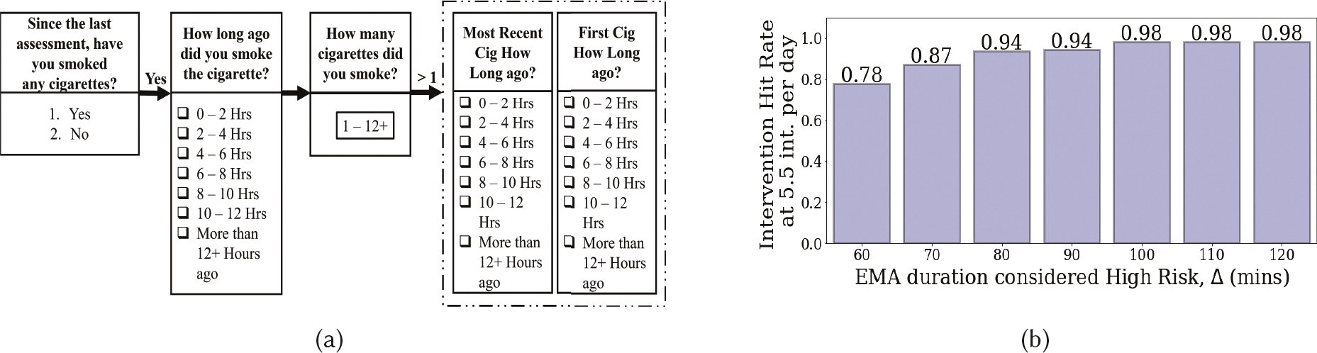
(a) Shows the EMA items corresponding to smoking report by individuals, (b) Intervention Hit Rate at 5.5 int. per day when considering a certain duration of EMA response as positive lapse.

As Figure 7a shows, participants indicate a 2-hour time window. When an EMA report of lapse is missed by puffMarker, we are unable to determine the precise moment of lapse and can only locate it in a 2-hour lapse window. Therefore, these labels are not used in training the models. In the absence of precise lapse moment, we consider the entire lapse window as the potential lapse time. For example, if at time t, a participant reports smoking a cigarette ‘4 – 6 Hours’ ago, we label t − 6 Hours to t − 4 Hours as containing a smoking event. The actual lapse event may occur anywhere in a specific lapse window, and hence the high-risk moments (that are assumed to precede a lapse) may occur at different portions of the 2-hour lapse window.

We adopt the following approach for computing the intervention hit rate for EMA-reported lapses. Let t_int denote the time when the estimated risk produced by the pre-trained mRisk model crosses a prespecified threshold (corresponding to an expected 5.5 interventions per day) and triggers an intervention. Let [t_EMA, t_EMA + 2H] denote the lapse window based on the participant’s EMA response. We say that the intervention delivered at time t_int has preceded a lapse if the prediction window [t_int, t_int + P_w] has an overlap with [t_EMA, t_EMA + Δ]. Here, Δ denotes the duration of time since the start of the 2-hour lapse window considered as high risk. If Δ = 60 minutes, then only the first hour of the 2-hour lapse window is considered to be high-risk. If Δ = 120 minutes, then the entire lapse window is considered high-risk. We assume that risk is high prior to a lapse and low afterwards, which is confirmed by our subsequent analysis (see Section 7.5).

We use 2-hour lapse windows that have risk scores available from the mRisk model at least 30 minutes (depending upon the availability of sensor data, including imputed data for short periods of missing sensor data). This results in a total of 615 lapse windows reported in 336 EMA’s that are used in this analysis.

We vary the value of Δ from 60 to 120 minutes and report the intervention hit rate in Figure 7b corresponding to 5.5 interventions per day. We observe that IHR increases from 0.78 and saturates at 0.98 for Δ = 100 minutes, indicating that most high-risk moments are contained within the first 100 minutes of the 2-hour lapse window. As the actual lapse moment and the actual high-risk moment may vary from instance to instance, the IHR reported here may represent an overestimation. Nevertheless, this analysis shows that the mRisk model may enable the delivery of an intervention prior to most self-reported lapses, even at the rate of 5.5 interventions per day.

7.5. Rise/Fall in Risk Levels Produced by mRisk Before/After Lapse Moments

As the mRisk model produces a continuous risk score, we visually analyze the rise and fall in the risk scores before and after lapse moments. We first apply the mRisk model post-facto on daylong data from a participant in Figure 8a. The moment of lapse from puffMarker is shown together with the time when the accompanying self-report of lapse was recorded. We make several observations.

Fig. 8.

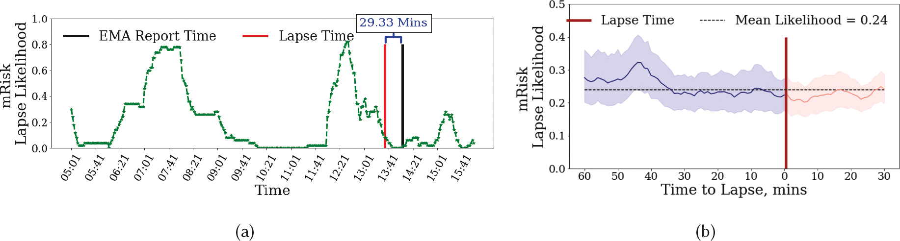
Lapse Likelihood produced by the DDHI model with lapse, intervention and EMA report times shown with vertical lines. We only include those EMAs in which the participants confirmed that the last time they smoked was 0–2 hours ago.

First, we observe that for the case when both detected and reported lapse are available (see Figure 8a), the reported time is 29.33 minutes after the actual lapse in this instance. In other instances, this time gap may be higher or lower. This ambiguity in determining the actual timing of lapse makes it difficult to use self-reported lapses (not supported by sensor-based detection) for model training or testing.

Second, in Figure 8a the lapse is preceded by a high-risk episode as estimated by the mRisk model. We further observe that as time gets closer to the lapse moment, the risk decreases. We also observe that once lapse occurs, the risk falls further, perhaps due to satiation of smoking urge.

Third, we observe two high-risk windows in the entire day. The mRisk model can guide the delivery of an intervention prior to the risk reaching its peak during both the high-risk episodes.

Figure 8a only shows the variation in risk score around one lapse moment for a single participant. To see if there is a general pattern of risk rising prior to lapse and falling immediately before and after the lapse moment, we aggregate the risk scores across all lapse moments from all participants. Figure 8b shows the mean lapse risk (with a confidence interval of 90%) before and after a smoking lapse. The mean risk score is also plotted. We observe that generally, the risk score is around the mean level. But, it rises and peaks around 44 minutes prior to a smoking lapse. The risk then decreases as the time approaches the lapse moment, falling below the mean level at the time of lapse, and falling even further after the lapse moment. We note that even though the observed variability may diminish when data from different lapse instances are pooled, due to the risk peaking at different times for different lapse instances, we still see a robust pattern at the population scale.

7.6. Understanding the Role of Context in Estimating Lapse Risk via Model Explanations

For the mRisk model to be trusted by intervention researchers [14], we analyze the behavior of the mRisk model in terms of the influence of the three major sensor-derived contexts (i.e., stress, activity, and location) on the lapse risk. We utilize the SHapley Additive exPlanations (SHAP), a game theory-based algorithm that can be employed to explain global and local feature importance for a fitted machine learning model [42]. SHAP explains a prediction by assuming that each feature value of the instance is a player in a game and the final prediction is a payout. Based on coalition game theory principles, the algorithm assigns payouts to players depending upon their contribution to the total payout. Players cooperate in the coalition and receive specific profits. In our case, the payout is the prediction of the risk of lapse for a single instance. The profit is the actual prediction for this instance minus the average prediction across all instances. The Shapley value is the weighted marginal contribution of a feature across all the possible coalitions. Features with large absolute Shapley values are more important.

We approximate the Shapley values for each input node of the DRES using the Deep SHAP method proposed in [42]. Deep SHAP builds upon DeepLIFT [68], which is a local additive feature attribution method for approximating the conditional expectations of SHAP values using a collection of background samples (training data, see [11] for details). Using Deep SHAP, we first obtain the Shapley values of each input instance (n_t × n_f, n_f = 62) of the mRisk model. We then average the Shapley values of each feature along the time axis. Finally, Shapley values of all instances across all participants are aggregated to interpret the collective impact of the input features on the model (i.e., global feature importance).

7.6.1. Observations from Global Feature Importance.

Figure 9 shows the impact of top 15 features on the mRisk model output, ranked by their Shapley values, averaged over all iterations. The top features are distributed across multiple contexts — visiting smoking spots, stress, activity, and hour of day. The most influential feature (time since last visit to smoking spot and fraction of stay duration at smoking spots until obs) indicate that exposures to smoking spots influences lapse risk. Average duration of activity events until obs also has significant influence. We hypothesize that spending more time moving around increases the chance of exposure to environmental cues of smoking, which may increase the risk of lapse.

Fig. 9.

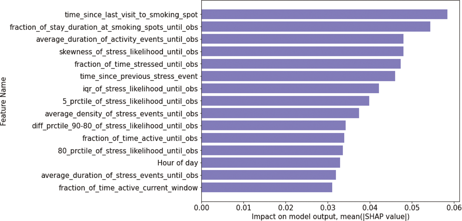
Global Feature Importance showing top 10 features for DRES model using Deep SHAP.

We observe that 9 out of the 15 features are related to stress. These include skewness of stress likelihood until obs, fraction of time stressed until obs, and average density of stress events until obs. We hypothesize that frequency and duration of high-stress likelihood so far in the day influences the risk of lapse. We also observe the event-of-influence features, which encode the temporal dynamics of recent contexts, outrank the continuous inference features. This observation underscores the importance of suitably representing the events-of-influence time series in a deep modeling framework that utilizes these contexts for learning.

8. RELATED WORKS

Our work on predicting the imminent risk of adverse behaviors is related to and builds upon several prior works.

Research on Predicting the Risk of Adverse Events:

Several works have been done on predicting the risk of adverse clinical/health events such as mortality [5, 19, 20, 71], ICU admission[79, 82], disease diagnosis [2, 13, 18, 28, 78], clinical sepsis [17, 62], property fire hazards [43, 69, 73], flood [47], road accidents [12, 44, 45], and wildfire [21, 57]. In each of these cases, both negative and positive labels were available and used for model training and the phenomena studied were better understood in terms of the influence of the input variables.

Research on Identifying Risk Factors of Adverse Behaviors from Self-Reports:

The risk factors or the determinants of lapse behaviors have been studied extensively via self-reports. These factors have been categorized into two broad categories [38]. First are the covert antecedents or the physiological/emotional states such as stress, craving/urge, and self-regulatory capacity. For instance, elevated stress levels and low self-regulatory capacity may increase the risk of a smoking lapse [23, 66, 67]. Similarly, enhanced negative affect, low resilience, and self-esteem usually lead to impulsive unhealthy eating in young adults [30]. Second, are the environmental or social cues such as being in a context that is conducive to a lapse behavior. For instance, it has been found that being at a place where cigarettes are available or seeing others smoke are significantly associated with the increase in vulnerability to a smoking lapse [64, 66]. In addition, impulsive binge drinking has been found to be significantly associated with peer-family influence, companion-competition, and interactions at social gatherings [29]. Self-reports do not provide a precise timing of the lapse events and hence can’t be used for developing continuous risk estimates. Further, methods used for analyzing self-reports are not applicable to analyzing noisy and continuous sensor data. But, these works motivate the formulation of the mRisk model. Specifically, we utilize the passive and continuous streams of some of the associated physiological and situational risk factors as inputs into the mRisk model to predict the imminent risk of lapse behaviors.

Research on Detection of Risk Factors Using Mobile Sensors:

For the continuous estimation of the imminent risk of adverse behaviors in the natural environment of individuals, passive and continuous detection of the associated risk factors using mobile and wearable sensors is necessary. Fortunately, recent advances in mobile and wearable sensing technologies have enabled the development of computational models for the continuous detection of the risk factors. For instance, these works [6, 27, 75] have been able to detect stress and depression from wearable physiological sensors (ECG and respiration) and smartphone-based GPS sensor data, respectively. Other works have been developed to continuously estimate the craving/urge for addictive behaviors such as cigarette smoking [8], alcohol consumption [51], and cocaine intake [22]. Finally, recent works have developed models to detect the environmental cues that are conducive to adverse behaviors. For instance, a recent work [9] introduced and defined contexts that are conducive to adverse behaviors as ‘opportunity’ contexts and developed a computational model for the reliable detection of the smoking ‘opportunity’ contexts using GPS and activity data. We leverage these works to extract psychological, behavioral, and environmental risk factors and use them as multidimensional input to the mRisk model.

Research on Predicting Mood and Behaviors:

Several recent works have demonstrated the feasibility of predicting mood and behaviors from self-report and mobile sensor data [39, 50, 70, 74, 76, 80]. For instance, [50] developed a model to predict the onset of excessive fatigue during an outdoor running session using inertial sensor data. Another work [70] presents a recurrent neural network-based model to forecast the depressive mood of individuals in the coming n days based on the user’s history during the last k days. Other works have proposed deep neural network frameworks [39, 80] to perform personalized prediction of self-reported mood, health, and stress scores using physiological and behavioral information from continuous sensor data. A closely related to ours is [74] that detects mood instabilities in patients who have schizophrenia using activity, location, and audio data passively collected from mobile sensors. A subsequent work [76] developed a model to predict relapse episodes in patients who have schizophrenia using 30 days of symptom trajectory data.

We complement these works by presenting the first model to continuously estimate the risk of smoking lapse using noisy mobile sensor data with incomplete and positive-only labels and no confirmed negative labels.

9. DISCUSSION, LIMITATIONS, AND FUTURE WORKS

Although this work uses a specific application of smoking lapse and a specific real-world dataset, the many interesting challenges encountered in modeling and the proposed ideas to address them may be applicable in the continuous estimation of risk in related domains such as the risk of lapse when quitting excessive drinking, abstaining from addictive substances (e.g., cocaine), controlling overeating, overcoming suicide attempts, among others. Like smoking, each of these adverse behaviors occurs in the natural environment. Similar to smoking lapses, they are influenced by both internal states and external cues. Mobile sensor data can passively track risk factors for each of these, but they are likely to be similarly noisy. Finally, the timing of a subset of adverse events may be obtained, but getting unambiguous negative labels is similarly difficult.

The mRisk model proposes a new end-to-end framework for model development that may be adaptable to continuously estimate the risk of other adverse behaviors. It presents approaches to incorporate the influence of both recent and past events captured from imperfect machine learning models applied to noisy sensor data and proposes a new loss function with customizable parameters to train a model for continuous risk estimation. It also proposes approaches for evaluating modeling choices in the absence of unambiguous negative labels by using the limiting of intervention burden in place of negative models to guide the model optimization. It also shows an approach for evaluating the expected utility of such risk models in a simulated delivery of interventions.

9.1. Key New Insights

For estimating the risk for smoking lapse in newly abstinent smokers, the mRisk model led to several new insights. First, it helped determine the proportion of unlabeled data that is likely to represent a high-risk. Second, we find that determining the personal smoking spots during the pre-quit period and using them in risk estimation can lead to substantial improvement in the model performance. Third, via visual analysis of the continuous risk estimates produced by the mRisk model, we find that lapse risk peaks about 44 minutes prior to an impending lapse, providing sufficient opportunity to intervene. Fourth, we find that 85% of lapses can potentially be intervened upon with only 5.5 interventions per day. Finally, via explanation, we find that recent exposure to smoking spots has a large influence on the lapse risk together with being physically active and a high likelihood of recent stress.

9.2. Limitations and Future Works

This work is only a first step towards continuous estimation of risk for adverse behaviors using mobile sensors that can be used in real-life field settings. It has several limitations that present exciting opportunities for future research for both computing and health researchers. First, many smoking lapses captured in EMAs could not be used in our model development or evaluation as they were not detected by puffMarker, preventing a precise determination of the time of lapse. The EMAs locate the past smoking events (sometimes more than one) within a 2-hour long window. This does not allow a determination of which segments of sensor data within this 2-hour window correspond to moments prior to a lapse and can be labeled high-risk. Future work can explore novel ideas to make use of these temporally-imprecise label sources to further improve the model.

Second, future work can also explore ways to identify moments of low risk via EMA responses and use them to train the usual two-class models. Third, this work shows the direct applicability of the presented mRisk framework to estimate the risk of smoking lapse. Applying it to other datasets of smoking cessation may require adaptation of some parameters such as the ϵ value in the RP loss function and the choice of percentiles in deciding the value of P. Future work can explore how well the mRisk framework may be used to estimate the risk of other adverse behaviors (e.g., alcoholism, drug addiction, etc.) that also have noisy data and incomplete and positive-only labels.

Fourth, the mRisk model achieves a good recall (IHR) using only the stress, location, and activity features. Future work can boost the performance further by supplementing them with craving, self-efficacy, presence of other cues such as noisy locations, graffiti, and other situational indicators that may affect the risk of lapse. Another idea to improve the model performance may be to use self-report data from EMAs in the context of research studies that collect EMAs for other purposes. Fifth, our simulation of intervention delivery only uses an intervention gap to avoid fatigue from frequent interventions. Future work can improve its real-life applicability by incorporating other constraints such as users’ receptivity [37] and availability [59].

Sixth, our evaluations assume that interventions can be delivered as soon as high-risk moments are detected if permitted by other constraints. But, how the detection of high-risk moments can be used to deliver the most efficacious intervention requires a just-in-time-adaptive-intervention (JITAI) optimization trials (e.g., micro-randomized trial) [36] to determine the best conditions (e.g., high-risk, moderate risk, or low-risk) and the best corresponding combination of the intervention content, mode of delivery, and the adaptation mechanisms for personalizing the intervention to the individual based on his/her contexts. Seventh, risk scores produced by mRisk can potentially be used to evaluate the impact of interventions that target stress reduction, location exposure via geofences, nicotine medications, and others in reducing the lapse risk. Eight, the risk scores along with the driving factors can be presented to newly abstinent smokers at the end of the day to help them understand their vulnerabilities better. Finally, mRisk is an offline model, computed only from observational data after data has already been collected. However, to be widely used for sensor-triggered mobile intervention during micro-randomized trials, future work can implement an online version of the mRisk model to run on wearable devices or smartphones. Only then can the model be used to trigger real-time mobile interventions based on the online prediction of the risk of a lapse in the natural environment of the participants. These make for exciting future research agenda for the computing and health research community.

10. CONCLUSION

The majority of chronic diseases can be prevented or better managed by improving health-related behaviors. Automated detection of risky contexts via mobile (and wearable) devices provides a new opportunity to improve the success rate with behavior modification. But, the overall risks depend on a multitude of factors, including internal states, personal behaviors, and environmental cues. Many of these factors can now be detected by applying machine learning models on data collected by wearable devices and smartphones. But, the challenge is noise in the data collected and lack of unambiguous labels of low- and high-risk moments. This work provides a new framework to estimate the overall risk of adverse behaviors despite noisy data, no labels of low-risk states, and availability of only a subset of high-risk states. It shows the successful application of this model on smoking cessation dataset, opening the doors for exciting new opportunities in the design and delivery of efficacious behavioral interventions to help people live healthier lives.

A. APPENDIX

A.1. Positive-Unlabeled Learning

Traditional supervised classifiers usually need clearly marked positive and negative samples for training. Therefore, such methods become unsuitable when only positively-labeled and unlabeled training data are available. For such scenarios, a different learning framework called Positive-Unlabeled (PU) have been developed [4, 31].

In the classical PU learning algorithm [15] a standard binary classifier is trained from the nontraditional positive-unlabeled setup. They show that a classifier trained on positive unlabeled examples learns probabilities that differ from the true conditional probabilities of being positive by only a constant factor, equivalent to the constant probability that a positive sample is labeled in the given data set. Using different weights for false Negatives vs. false Positives in training have also been proposed for solving the classical PU-learning problem. For instance, the biased SVM approach in [40] solves the PU-learning problem by using soft margin SVM while giving high weights to false negative errors and low weights to false positive errors. However, these classic PU learning algorithms work only under the strong assumption that the set of labeled examples is a uniformly random subset of the positive examples (or the positive-label samples are ‘selected completely at random’ (SCAR)).

For scenario such as ours where the SCAR assumption does not hold, the PU-bagging or ensemble PU learning have been proposed [46]. The idea is to estimate a series of classifiers on datasets obtained by perturbing the original training set through bootstrap re-sampling with replacement, and to combine these classifiers by some aggregation technique. In each iteration, the base model is trained with all the high-risk labelled instances as positive and a random sample of the unlabeled class as negative class. We optimize the model by computing the cross entropy loss and the proposed RP-loss function. At each iteration, we keep the ratio of positive to sampled unlabeled instances balanced and apply the model trained on the test set to estimate the out-of-bag score (which is lapse likelihood in our case). The average out-of-bag score of k (= 100) such models act as the final risk score we obtain in the test set. We employ leave-one-participant-out-cross-validation (LOPOCV) to segment our dataset and train models. In each cross-validation fold, we segment one participant’s data as a test set and consider the rest as train set. We train an ensemble PU-Bagging model using the train set and apply it on the test set to obtain the lapse likelihood time-series for that participant.

A.2. Intervention Hit Rate (IHR)

Intervention Hit Rate (IHR) measures the probability that an intervention opportunity is provided by mRisk ahead of each lapse event, i.e., within our prediction window (P_w). More formally, we first choose a value for risk threshold, T_L = c to achieve a desired frequency of interventions per day. An intervention opportunity at time t is created if the risk produced by mRisk, r(t) exceeds c and at least I_G (intervention gap) minutes have elapsed from the most recent intervention moment. Let $I(u)=\left\{t_1^i(u),t_2^i(u),t_3^i(u),\dots \right\}$ be the set containing the timings of interventions for a user (u). Let $L(u)=\left\{t_1^l(u),t_2^l(u),t_3^l(u),\dots \right\}$ be the precise time of a lapse events for user u (confirmed by EMA and Puffmarker). We consider the lapse event at time $t_k^l(u)$ to be intervened (or covered or hit) if $\exists j:t_j^i(u)\le t_k^l(u):t_k^l(u)-t_j^i(u)\le P_w$. The IHR can then be defined as

$$\frac{{\sum }_u\left|\forall k:\exists j:t_j^i(u)\le t_k^l(u):t_k^l(u)-t_j^i(u)\le P_w\right|}{{\sum }_u\left|L(u)\right|}.$$

We note that $t_j^i-t_{j+1}^i>I_G$, i.e., no successive interventions are at least I_G minutes apart. Therefore, there exists a unique j for each lapse moment, if I_G ≥ P_w.

REFERENCES

- [1].Accessed February, 2022. CDC: Smoking is the leading cause of preventable death. https://www.cdc.gov/tobacco/data_statistics/fact_sheets/fast_facts/index.htm
- [2].Bai Tian, Zhang Shanshan, Egleston Brian L, and Vucetic Slobodan. 2018. Interpretable representation learning for healthcare via capturing disease progression through time. In Proceedings of the 24th ACM SIGKDD International Conference on Knowledge Discovery & Data Mining. 43–51. [DOI] [PMC free article] [PubMed] [Google Scholar]
- [3].Baytas Inci M, Xiao Cao, Zhang Xi, Wang Fei, Jain Anil K, and Zhou Jiayu. 2017. Patient subtyping via time-aware lstm networks. In Proceedings of the 23rd ACM SIGKDD international conference on knowledge discovery and data mining. 65–74. [Google Scholar]
- [4].Bekker Jessa and Davis Jesse. 2020. Learning from positive and unlabeled data: A survey. Machine Learning 109, 4 (2020), 719–760. [Google Scholar]
- [5].Bhattacharya Sakyajit, Rajan Vaibhav, and Shrivastava Harsh. 2017. ICU mortality prediction: a classification algorithm for imbalanced datasets. In Proceedings of the AAAI Conference on Artificial Intelligence, Vol. 31. [Google Scholar]
- [6].Canzian Luca and Musolesi Mirco. 2015. Trajectories of depression: unobtrusive monitoring of depressive states by means of smartphone mobility traces analysis. In Proceedings of the 2015 ACM international joint conference on pervasive and ubiquitous computing. ACM, 1293–1304. [Google Scholar]
- [7].Chatterjee Soujanya. 2021. Machine Learning Models for Predicting the Imminent Risk of Impulsive Behaviors Using mHealth Sensors. [Google Scholar]
- [8].Chatterjee Soujanya, Hovsepian Karen, Sarker Hillol, Saleheen Nazir, Mustafa al’Absi Gowtham Atluri, Ertin Emre, Lam Cho, Lemieux Andrine, Nakajima Motohiro, et al. 2016. mCrave: Continuous estimation of craving during smoking cessation. In Proceedings of the 2016 ACM International Joint Conference on Pervasive and Ubiquitous Computing. ACM, 863–874. [DOI] [PMC free article] [PubMed] [Google Scholar]
- [9].Chatterjee Soujanya, Moreno Alexander, Lizotte Steven Lloyd, Akther Sayma, Ertin Emre, Fagundes Christopher P, Lam Cho, Rehg James M, Wan Neng, Wetter David W, et al. 2020. SmokingOpp: Detecting the Smoking’Opportunity’Context Using Mobile Sensors. Proceedings of the ACM on Interactive, Mobile, Wearable and Ubiquitous Technologies 4, 1 (2020), 1–26. [DOI] [PMC free article] [PubMed] [Google Scholar]
- [10].Che Zhengping, Purushotham Sanjay, Cho Kyunghyun, Sontag David, and Liu Yan. 2018. Recurrent neural networks for multivariate time series with missing values. Scientific reports 8, 1 (2018), 1–12. [DOI] [PMC free article] [PubMed] [Google Scholar]
- [11].Chen Hugh, Lundberg Scott, and Lee Su-In. 2021. Explaining models by propagating Shapley values of local components. In Explainable AI in Healthcare and Medicine. Springer, 261–270. [Google Scholar]
- [12].Chen Quanjun, Song Xuan, Yamada Harutoshi, and Shibasaki Ryosuke. 2016. Learning deep representation from big and heterogeneous data for traffic accident inference. In Proceedings of the AAAI Conference on Artificial Intelligence, Vol. 30. [Google Scholar]
- [13].Choi Edward, Schuetz Andy, Stewart Walter F, and Sun Jimeng. 2017. Using recurrent neural network models for early detection of heart failure onset. Journal of the American Medical Informatics Association 24, 2 (2017), 361–370. [DOI] [PMC free article] [PubMed] [Google Scholar]
- [14].Doshi-Velez Finale and Kim Been. 2017. Towards a rigorous science of interpretable machine learning. arXiv preprint arXiv:1702.08608 (2017). [Google Scholar]
- [15].Elkan Charles and Noto Keith. 2008. Learning classifiers from only positive and unlabeled data. In Proceedings of the 14th ACM SIGKDD international conference on Knowledge discovery and data mining. 213–220. [Google Scholar]
- [16].Ertin Emre, Stohs Nathan, Kumar Santosh, Raij Andrew, al’Absi Mustafa, and Shah Siddharth. 2011. AutoSense: unobtrusively wearable sensor suite for inferring the onset, causality, and consequences of stress in the field. In Proceedings of the 9th ACM Conference on Embedded Networked Sensor Systems. ACM, 274–287. [Google Scholar]
- [17].Futoma Joseph, Hariharan Sanjay, and Heller Katherine. 2017. Learning to detect sepsis with a multitask Gaussian process RNN classifier. In International Conference on Machine Learning. PMLR, 1174–1182. [Google Scholar]
- [18].Futoma Joseph, Hariharan Sanjay, Heller Katherine, Sendak Mark, Brajer Nathan, Clement Meredith, Bedoya Armando, and O’Brien Cara. 2017. An improved multi-output gaussian process rnn with real-time validation for early sepsis detection. In Machine Learning for Healthcare Conference. PMLR, 243–254. [Google Scholar]
- [19].Gao Yue, Cai Guang-Yao, Fang Wei, Li Hua-Yi, Wang Si-Yuan, Chen Lingxi, Yu Yang, Liu Dan, Xu Sen, Cui Peng-Fei, et al. 2020. Machine learning based early warning system enables accurate mortality risk prediction for COVID-19. Nature communications 11, 1 (2020), 1–10. [DOI] [PMC free article] [PubMed] [Google Scholar]
- [20].Ghassemi Marzyeh, Pimentel Marco, Naumann Tristan, Brennan Thomas, Clifton David, Szolovits Peter, and Feng Mengling. 2015. A multivariate timeseries modeling approach to severity of illness assessment and forecasting in ICU with sparse, heterogeneous clinical data. In Proceedings of the AAAI conference on artificial intelligence, Vol. 29. [PMC free article] [PubMed] [Google Scholar]
- [21].Gholami Shahrzad, Kodandapani Narendran, Wang Jane, and Ferres Juan Lavista. 2021. Where there’s Smoke, there’s Fire: Wildfire Risk Predictive Modeling via Historical Climate Data. In Annual Conference on Innovative Applications of Artificial Intelligence (IAAI). [Google Scholar]
- [22].Gullapalli Bhanu Teja, Natarajan Annamalai, Angarita Gustavo A, Malison Robert T, Ganesan Deepak, and Rahman Tauhidur. 2019. On-body sensing of cocaine craving, euphoria and drug-seeking behavior using cardiac and respiratory signals. Proceedings of the ACM on Interactive, Mobile, Wearable and Ubiquitous Technologies 3, 2 (2019), 1–31.34164595 [Google Scholar]
- [23].Gwaltney Chad J, Shiffman Saul, Balabanis Mark H, and Paty Jean A. 2005. Dynamic self-efficacy and outcome expectancies: prediction of smoking lapse and relapse. Journal of abnormal psychology 114, 4 (2005), 661. [DOI] [PubMed] [Google Scholar]
- [24].Hnat Timothy, Hossain Syed Monowar, Ali Nasir, Carini Simona, Condie Tyson, Sim Ida, Srivastava Mani B, and Kumar Santosh. 2017. mCerebrum and Cerebral Cortex: A Real-time Collection, Analytic, and Intervention Platform for High-frequency Mobile Sensor Data.. In AMIA. [Google Scholar]
- [25].Hossain S, Ali A, Rahman M, Ertin E, Epstein D, Kennedy A, Preston K, Umbricht A, Chen Y, and Kumar S. 2014. Identifying Drug (Cocaine) Intake Events from Acute Physiological Response in the Presence of Free-living Physical Activity. In ACM IPSN. 71–82. [PMC free article] [PubMed] [Google Scholar]
- [26].Hossain Syed Monowar, Hnat Timothy, Saleheen Nazir, Nasrin Nusrat Jahan, Noor Joseph, Ho Bo-Jhang, Condie Tyson, Srivastava Mani, and Kumar Santosh. 2017. mCerebrum: A Mobile Sensing Software Platform for Development and Validation of Digital Biomarkers and Interventions. In Proceedings of the 15th ACM Conference on Embedded Network Sensor Systems. ACM, 7. [DOI] [PMC free article] [PubMed] [Google Scholar]
- [27].Hovsepian K, al’Absi M, Ertin E, Kamarck T, Nakajima M, and Kumar S. 2015. cStress: towards a gold standard for continuous stress assessment in the mobile environment. In ACM UbiComp. 493–504. [DOI] [PMC free article] [PubMed] [Google Scholar]
- [28].Hyland Stephanie L, Faltys Martin, Hüser Matthias, Lyu Xinrui, Gumbsch Thomas, Esteban Cristóbal, Bock Christian, Horn Max, Moor Michael, Rieck Bastian, et al. 2020. Early prediction of circulatory failure in the intensive care unit using machine learning. Nature medicine 26, 3 (2020), 364–373. [DOI] [PubMed] [Google Scholar]
- [29].Ichiyama Michael A and Kruse Marc I. 1998. The social contexts of binge drinking among private university freshmen. Journal of Alcohol and Drug Education 44, 1 (1998), 18. [Google Scholar]
- [30].Izydorczyk Bernadetta, Sitnik-Warchulska Katarzyna, Lizińczyk Sebastian, and Lipiarz Adrianna. 2019. Psychological predictors of unhealthy eating attitudes in young adults. Frontiers in psychology 10 (2019), 590. [DOI] [PMC free article] [PubMed] [Google Scholar]
- [31].Jaskie Kristen and Spanias Andreas. 2019. Positive and unlabeled learning algorithms and applications: A survey. In 2019 10th International Conference on Information, Intelligence, Systems and Applications (IISA). IEEE, 1–8. [Google Scholar]
- [32].Kapoor Ashish and Horvitz Eric. 2008. Experience sampling for building predictive user models: a comparative study. In Proceedings of the SIGCHI Conference on Human Factors in Computing Systems. 657–666. [Google Scholar]
- [33].Tetik Burcu Kayhan, Tekinemre Işılay Gedik, and Taş Servet. 2021. The effect of the COVID-19 pandemic on smoking cessation success. Journal of Community Health 46, 3 (2021), 471–475. [DOI] [PMC free article] [PubMed] [Google Scholar]
- [34].Kenford Susan L, Fiore Michael C, Jorenby Douglas E, Smith Stevens S, Wetter David, and Baker Timothy B. 1994. Predicting smoking cessation: who will quit with and without the nicotine patch. Jama 271, 8 (1994), 589–594. [DOI] [PubMed] [Google Scholar]
- [35].Kirchner Thomas R, Shiffman Saul, and Wileyto E Paul. 2012. Relapse dynamics during smoking cessation: recurrent abstinence violation effects and lapse-relapse progression. Journal of abnormal psychology 121, 1 (2012), 187. [DOI] [PMC free article] [PubMed] [Google Scholar]
- [36].Klasnja Predrag, Eric B Hekler Saul Shiffman, Boruvka Audrey, Almirall Daniel, Tewari Ambuj, and Murphy Susan A. 2015. Microrandomized trials: An experimental design for developing just-in-time adaptive interventions. Health Psychology 34, S (2015), 1220. [DOI] [PMC free article] [PubMed] [Google Scholar]
- [37].Künzler Florian, Mishra Varun, Kramer Jan-Niklas, Kotz David, Fleisch Elgar, and Kowatsch Tobias. 2019. Exploring the state-of-receptivity for mhealth interventions. Proceedings of the ACM on Interactive, Mobile, Wearable and Ubiquitous Technologies 3, 4 (2019), 1–27. [DOI] [PMC free article] [PubMed] [Google Scholar]
- [38].Larimer Mary E and Marlatt G Alan. 2004. Relapse prevention: An overview of Marlatt’s cognitive-behavioral model. Psychosocial treatments (2004), 11–28. [PMC free article] [PubMed] [Google Scholar]
- [39].Li Boning and Sano Akane. 2020. Extraction and Interpretation of Deep Autoencoder-based Temporal Features from Wearables for Forecasting Personalized Mood, Health, and Stress. Proceedings of the ACM on Interactive, Mobile, Wearable and Ubiquitous Technologies 4, 2 (2020), 1–26.35846237 [Google Scholar]
- [40].Liu Bing, Dai Yang, Li Xiaoli, Lee Wee Sun, and Yu Philip S. 2003. Building text classifiers using positive and unlabeled examples. In Third IEEE international conference on data mining. IEEE, 179–186. [Google Scholar]
- [41].Liu Bing, Lee Wee Sun, Yu Philip S, and Li Xiaoli. 2002. Partially supervised classification of text documents. In ICML, Vol. 2. Sydney, NSW, 387–394. [Google Scholar]
- [42].Lundberg Scott M and Lee Su-In. 2017. A unified approach to interpreting model predictions. In Proceedings of the 31st international conference on neural information processing systems. 4768–4777. [Google Scholar]
- [43].Madaio Michael, Chen Shang-Tse, Haimson Oliver L, Zhang Wenwen, Cheng Xiang, Hinds-Aldrich Matthew, Horng Chau Duen, and Dilkina Bistra. 2016. Firebird: Predicting fire risk and prioritizing fire inspections in Atlanta. In Proceedings of the 22nd ACM SIGKDD International Conference on Knowledge Discovery and Data Mining. 185–194. [Google Scholar]
- [44].Moosavi Sobhan, Samavatian Mohammad Hossein, Nandi Arnab, Parthasarathy Srinivasan, and Ramnath Rajiv. 2019. Short and long-term pattern discovery over large-scale geo-spatiotemporal data. In Proceedings of the 25th ACM SIGKDD International Conference on Knowledge Discovery & Data Mining. 2905–2913. [Google Scholar]
- [45].Moosavi Sobhan, Samavatian Mohammad Hossein, Parthasarathy Srinivasan, Teodorescu Radu, and Ramnath Rajiv. 2019. Accident Risk Prediction based on Heterogeneous Sparse Data: New Dataset and Insights. In Proceedings of the 27th ACM SIGSPATIAL International Conference on Advances in Geographic Information Systems. 33–42. [Google Scholar]
- [46].Mordelet Fantine and Vert J-P. 2014. A bagging SVM to learn from positive and unlabeled examples. Pattern Recognition Letters 37 (2014), 201–209. [Google Scholar]
- [47].Mosavi Amir, Ozturk Pinar, and Chau Kwok-wing. 2018. Flood prediction using machine learning models: Literature review. Water 10, 11 (2018), 1536. [Google Scholar]
- [48].Nahum-Shani Inbal, Smith Shawna N, Spring Bonnie J, Collins Linda M, Witkiewitz Katie, Tewari Ambuj, and Murphy Susan A. 2018. Just-in-time adaptive interventions (JITAIs) in mobile health: key components and design principles for ongoing health behavior support. Annals of Behavioral Medicine 52, 6 (2018), 446–462. [DOI] [PMC free article] [PubMed] [Google Scholar]
- [49].Naughton Felix, Hopewell Sarah, Lathia Neal, Schalbroeck Rik, Brown Chloë, Mascolo Cecilia, McEwen Andy, and Sutton Stephen. 2016. A context-sensing mobile phone app (Q sense) for smoking cessation: a mixed-methods study. JMIR mHealth and uHealth 4, 3 (2016), e106. [DOI] [PMC free article] [PubMed] [Google Scholar]
- [50].De Beéck Tim Op, Meert Wannes, Schütte Kurt, Vanwanseele Benedicte, and Davis Jesse. 2018. Fatigue prediction in outdoor runners via machine learning and sensor fusion. In Proceedings of the 24th acm sigkdd international conference on knowledge discovery & data mining. 606–615. [Google Scholar]
- [51].Phan Thanh-Trung, Muralidhar Skanda, and Gatica-Perez Daniel. 2019. Drinks & crowds: Characterizing alcohol consumption through crowdsensing and social media. Proceedings of the ACM on Interactive, Mobile, Wearable and Ubiquitous Technologies 3, 2 (2019), 1–30.34164595 [Google Scholar]
- [52].Rahman Md Mahbubur, Bari Rummana, Ali Amin Ahsan, Sharmin Moushumi, Raij Andrew, Hovsepian Karen, Hossain Syed Monowar, Ertin Emre, Kennedy Ashley, Epstein David H, et al. 2014. Are we there yet?: Feasibility of continuous stress assessment via wireless physiological sensors. In ACM BCB. 479–488. [DOI] [PMC free article] [PubMed] [Google Scholar]
- [53].Reitzel Lorraine R, Cromley Ellen K, Li Yisheng, Cao Yumei, Mater Richard Dela, Mazas Carlos A, Cofta-Woerpel Ludmila, Cinciripini Paul M, and Wetter David W. 2011. The effect of tobacco outlet density and proximity on smoking cessation. American Journal of Public Health 101, 2 (2011), 315–320. [DOI] [PMC free article] [PubMed] [Google Scholar]
- [54].Rousseeuw Peter J. 1987. Silhouettes: a graphical aid to the interpretation and validation of cluster analysis. Journal of computational and applied mathematics 20 (1987), 53–65. [Google Scholar]
- [55].Saleheen Nazir, Ali Amin Ahsan, Hossain Syed Monowar, Sarker Hillol, Chatterjee Soujanya, Marlin Benjamin, Ertin Emre, al’Absi Mustafa, and Kumar Santosh. 2015. puffMarker: a multi-sensor approach for pinpointing the timing of first lapse in smoking cessation. In ACM UbiComp. 999–1010. [PMC free article] [PubMed] [Google Scholar]
- [56].Saleheen Nazir, Ullah Md Azim, Chakraborty Supriyo, Ones Deniz S, Srivastava Mani, and Kumar Santosh. 2021. WristPrint: Characterizing User Re-identification Risks from Wrist-worn Accelerometry Data. In Proceedings of the 2021 ACM SIGSAC Conference on Computer and Communications Security. 2807–2823. [DOI] [PMC free article] [PubMed] [Google Scholar]
- [57].Salehi Mahsa, Rusu Laura Irina, Lynar Timothy, and Phan Anna. 2016. Dynamic and robust wildfire risk prediction system: an unsupervised approach. In Proceedings of the 22nd ACM SIGKDD International Conference on Knowledge Discovery and Data Mining. 245–254. [Google Scholar]
- [58].Sarker Hillol, Hovsepian Karen, Chatterjee Soujanya, Nahum-Shani Inbal, Murphy Susan A, Spring Bonnie, Ertin Emre, Al’Absi Mustafa, Nakajima Motohiro, and Kumar Santosh. 2017. From markers to interventions: The case of just-in-time stress intervention. In Mobile health. Springer, 411–433. [Google Scholar]
- [59].Sarker H, Sharmin M, Ali A, Rahman M, Bari R, Hossain S, and Kumar S. 2014. Assessing the availability of users to engage in just-in-time intervention in the natural environment. In ACM UbiComp. 909–920. [DOI] [PMC free article] [PubMed] [Google Scholar]
- [60].Sarker Hillol, Tyburski Matthew, Rahman Md Mahbubur, Hovsepian Karen, Sharmin Moushumi, Epstein David H, Preston Kenzie L, Debra Furr-Holden C, Milam Adam, Nahum-Shani Inbal, et al. 2016. Finding significant stress episodes in a discontinuous time series of rapidly varying mobile sensor data. In Proceedings of the 2016 CHI conference on human factors in computing systems. 4489–4501. [DOI] [PMC free article] [PubMed] [Google Scholar]
- [61].Schroff Florian, Kalenichenko Dmitry, and Philbin James. 2015. Facenet: A unified embedding for face recognition and clustering. In Proceedings of the IEEE conference on computer vision and pattern recognition. 815–823. [Google Scholar]
- [62].Sheetrit Eitam, Nissim Nir, Klimov Denis, and Shahar Yuval. 2019. Temporal probabilistic profiles for sepsis prediction in the ICU. In Proceedings of the 25th ACM SIGKDD International Conference on Knowledge Discovery & Data Mining. 2961–2969. [Google Scholar]
- [63].Shiffman Saul. 2006. Reflections on smoking relapse research. Drug and alcohol review 25, 1 (2006), 15–20. [DOI] [PubMed] [Google Scholar]
- [64].Shiffman Saul, Balabanis Mark H, Gwaltney Chad J, Paty Jean A, Gnys Maryann, Kassel Jon D, Hickcox Mary, and Paton Stephanie M. 2007. Prediction of lapse from associations between smoking and situational antecedents assessed by ecological momentary assessment. Drug and alcohol dependence 91, 2–3 (2007), 159–168. [DOI] [PMC free article] [PubMed] [Google Scholar]
- [65].Shiffman Saul, Hickcox Mary, Paty Jean A, Gnys Maryann, Kassel Jon D, and Richards Thomas J. 1996. Progression from a smoking lapse to relapse: prediction from abstinence violation effects, nicotine dependence, and lapse characteristics. Journal of consulting and clinical psychology 64, 5 (1996), 993. [DOI] [PubMed] [Google Scholar]
- [66].Shiffman Saul, Paty Jean A, Gnys Maryann, Kassel Jon A, and Hickcox Mary. 1996. First lapses to smoking: within-subjects analysis of real-time reports. Journal of consulting and clinical psychology 64, 2 (1996), 366. [DOI] [PubMed] [Google Scholar]
- [67].Shiffman Saul and Waters Andrew J. 2004. Negative affect and smoking lapses: a prospective analysis. Journal of consulting and clinical psychology 72, 2 (2004), 192. [DOI] [PubMed] [Google Scholar]
- [68].Shrikumar Avanti, Greenside Peyton, and Kundaje Anshul. 2019. Learning Important Features Through Propagating Activation Differences. arXiv:cs.CV/1704.02685 [Google Scholar]
- [69].Walia Bhavkaran Singh, Hu Qianyi, Chen Jeffrey, Chen Fangyan, Lee Jessica, Kuo Nathan, Narang Palak, Batts Jason, Arnold Geoffrey, and Madaio Michael. 2018. A dynamic pipeline for spatio-temporal fire risk prediction. In Proceedings of the 24th ACM SIGKDD International Conference on Knowledge Discovery & Data Mining. 764–773. [Google Scholar]
- [70].Suhara Yoshihiko, Xu Yinzhan, and Pentland Alex’Sandy’. 2017. Deepmood: Forecasting depressed mood based on self-reported histories via recurrent neural networks. In Proceedings of the 26th International Conference on World Wide Web. 715–724. [Google Scholar]
- [71].Suresh Harini, Gong Jen J, and Guttag John V. 2018. Learning tasks for multitask learning: Heterogeneous patient populations in the icu. In Proceedings of the 24th ACM SIGKDD International Conference on Knowledge Discovery & Data Mining. 802–810. [Google Scholar]
- [72].Suresh Harini, Hunt Nathan, Johnson Alistair, Leo Anthony Celi Peter Szolovits, and Ghassemi Marzyeh. 2017. Clinical intervention prediction and understanding using deep networks. arXiv preprint arXiv:1705.08498 (2017). [Google Scholar]
- [73].Wang Qianru, Zhang Junbo, Guo Bin, Hao Zexia, Zhou Yifang, Sun Junkai, Yu Zhiwen, and Zheng Yu. 2019. CityGuard: citywide fire risk forecasting using a machine learning approach. Proceedings of the ACM on Interactive, Mobile, Wearable and Ubiquitous Technologies 3, 4 (2019), 1–21.34164595 [Google Scholar]
- [74].Wang Rui, Wang Weichen, Aung Min SH, Ben-Zeev Dror, Brian Rachel, Campbell Andrew T, Choudhury Tanzeem, Hauser Marta, Kane John, Scherer Emily A, et al. 2017. Predicting symptom trajectories of schizophrenia using mobile sensing. Proceedings of the ACM on Interactive, Mobile, Wearable and Ubiquitous Technologies 1, 3 (2017), 1–24. [Google Scholar]
- [75].Wang Rui, Wang Weichen, DaSilva Alex, Huckins Jeremy F, Kelley William M, Heatherton Todd F, and Campbell Andrew T. 2018. Tracking depression dynamics in college students using mobile phone and wearable sensing. Proceedings of the ACM on Interactive, Mobile, Wearable and Ubiquitous Technologies 2, 1 (2018), 1–26. [Google Scholar]
- [76].Wang Rui, Wang Weichen, Obuchi Mikio, Scherer Emily, Brian Rachel, Ben-Zeev Dror, Choudhury Tanzeem, Kane John, Hauser Martar, Walsh Megan, et al. 2020. On Predicting Relapse in Schizophrenia using Mobile Sensing in a Randomized Control Trial. In 2020 IEEE International Conference on Pervasive Computing and Communications (PerCom). IEEE, 1–8. [Google Scholar]
- [77].Xu Jiehui, Wang Jianmin, Long Mingsheng, et al. 2021. Autoformer: Decomposition transformers with auto-correlation for long-term series forecasting. Advances in Neural Information Processing Systems 34 (2021). [Google Scholar]
- [78].Xu Yanbo, Biswal Siddharth, Deshpande Shriprasad R, Maher Kevin O, and Sun Jimeng. 2018. Raim: Recurrent attentive and intensive model of multimodal patient monitoring data. In Proceedings of the 24th ACM SIGKDD international conference on Knowledge Discovery & Data Mining. 2565–2573. [Google Scholar]
- [79].Yoon Jinsung, Alaa Ahmed, Hu Scott, and Schaar Mihaela. 2016. ForecastICU: a prognostic decision support system for timely prediction of intensive care unit admission. In International Conference on Machine Learning. PMLR, 1680–1689. [Google Scholar]
- [80].Yu Han, Klerman Elizabeth B, Picard Rosalind W, and Sano Akane. 2019. Personalized wellbeing prediction using behavioral, physiological and weather data. In 2019 IEEE EMBS International Conference on Biomedical & Health Informatics (BHI). IEEE, 1–4. [Google Scholar]
- [81].Zhang Zhilu and Sabuncu Mert. 2018. Generalized cross entropy loss for training deep neural networks with noisy labels. Advances in neural information processing systems 31 (2018). [Google Scholar]
- [82].Zhao Zirun, Chen Anne, Hou Wei, Graham James M, Li Haifang, Richman Paul S, Thode Henry C, Singer Adam J, and Duong Tim Q. 2020. Prediction model and risk scores of ICU admission and mortality in COVID-19. PloS one 15, 7 (2020), e0236618. [DOI] [PMC free article] [PubMed] [Google Scholar]
- [83].Zheng Yu. 2015. Trajectory data mining: an overview. ACM Transactions on Intelligent Systems and Technology (TIST) 6, 3 (2015), 29. [Google Scholar]
- [84].Zhou Haoyi, Zhang Shanghang, Peng Jieqi, Zhang Shuai, Li Jianxin, Xiong Hui, and Zhang Wancai. 2021. Informer: Beyond efficient transformer for long sequence time-series forecasting. In Proceedings of AAAI. [Google Scholar]