Abstract
A tutorial introduction to Monte Carlo (MC) simulation of light propagation in biological tissues. MC statistical sampling is introduced, the basic design of a MC program is explained, and examples of application in biomedicine are presented.
1. Introduction
The penetration of light into and within a biological tissue is the key to many diagnostic and therapeutic uses of lasers and other light sources in medicine and biology. The dose of light experienced by a target structure within a tissue, eg., a blood vessel or a tumor, guides the irradiance and exposure time required for a particular photochemical, photothermal, or photomechanical effect. Understanding how photons propagate within and escape from a tissue is necessary for proper interpretation of optical diagnostic measurements. The field of biomedical optics and biophotonics is currently very actively using computer simulations of light transport to guide clinical protocols and develop optical tools for medicine and biology.
Monte Carlo (MC) simulations of light transport in media with absorption and scattering properties has long been an important tool in many fields. The MC method is a statistical sampling of probability density functions, and an early application was study of the movement of neutrons in fissile materials for nuclear reactions; see [1] for a history of early MC development. MC simulations have been widely used in astrophysical, atmospheric, oceanic, and now biomedical applications. This paper does not attempt a review of the field. Rather, this tutorial introduces MC to newcomers to the field. At its heart, MC is quite simple and demystifying the computation is a goal of the paper.
There have been many MC programs written by many investigators. Some recent examples are mcml [2], MCmatlab [3], and mcx [4]. Others have created websites that allow users to run simulations on-line, such as the Biophotonics Initiative [5], mcxspace [6], Cloud based Monte Carlo [7], and Multi-Scattering [8].
The paper begins with an introduction to Monte Carlo sampling, then discusses the basic structure of an MC program, and concludes with three example problems: (1) How does skin architecture affect skin color? (2) What exposure time is needed for photobiomodulation of the knee? (3) Will a pulsed laser treatment reach the bulb of a hair follicle?
2. Monte Carlo sampling
2.1. Concept
Monte Carlo sampling is the random sampling of a probability density function, p(x), to pick a value x. This section illustrates MC sampling using a bucket of marbles, then presents the general approach toward finding an analytic expression that uses a random number (RND) to pick a value of x. Two examples are given: (1) picking a stepsize for a photon to propagate before being scattered, and (2) picking a launch position for launching each photon as a large number of photons are delivered to a tissue as a collimated Gaussian beam.
Bucket of marbles
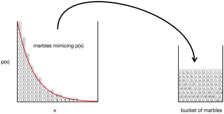
Consider a bucket that you are going to fill with a N marbles, for example N = 1000. Divide the range of x into discrete steps of x, for example 100 steps of size dx = 0.01 between 0 and 1. Calculate the corresponding discrete values of p(x) that correspond to each discrete value of x, where p(x) is a normalized probability density function. For each x value, write the value of x on a set of Np(x)dx marbles and place these marbles in the bucket. For example, if x = 0.2 and p(x) = , x = 1.8394, then Np(x)dx equals round((1000)(1.8394)(0.01)) = 18 marbles, on which you write the value 0.2 and place in the bucket. After doing this for all your steps of x, you now have a bucket filled with 1000 labeled marbles, but more are labeled with small values of x and fewer are labeled with large values of x, since p(x) is an exponential decay function.
Now proceed to sample p(x) by picking a marble from the bucket. The value on the marble is your x1. Put the marble back into the bucket, shake the bucket, and draw a second marble, yielding a new x1. Repeat. This process of sampling marbles in the bucket is a simple version of the Monte Carlo method. Figure 1 illustrates the concept of the bucket filled with marbles.
Fig. 1.
Monte Carlo sampling. On the left, marbles distributed as p(x) are labeled by their x value. On the right, the labeled marbles have filled a bucket. Randomly drawing a marble from the bucket yields a marble labeled by x.
Sampling diagram
Now consider using the Monte Carlo method to sample a generic probability density function p(x), normalized such that
| (1) |
The corresponding probability distribution function is F(x):
| (2) |
Now consider a random number generator that generates a random number RND. The p(RND) equals a constant 1 over the interval 0 to 1, since any value of RND has an equal chance. Consequently, F(RND) = RND, which is a linear increase from 0 to 1 with a slope of 1. To sample the p(x), equate the probability distribution functions, F(RND) = F(x), in other words, let F(x) = RND. Then solve for x to yield a new equation x = function(RND). Now, the sampling of p(x) uses a randomly generated to produces a value . This is a computational approach toward Monte Carlo sampling.
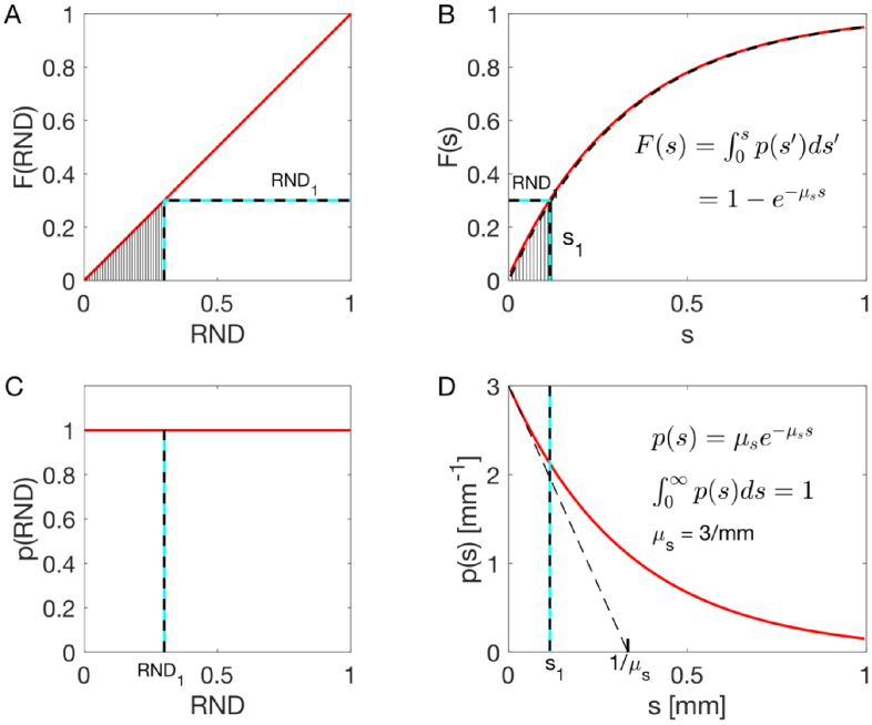
This strategy is illustrated in Fig. 2, using , which is the probability density function for the step size (s) a photon will take before being scattered. The p(s) is properly normalized (integral of p(s) from 0 to equals unity). The function F(s) is
| (3) |
Fig. 2.
Monte Carlo sampling of p(s) using a random number RND. A choice of connects to a value by equating the F(r) to RND. The hatched areas under the curves p(RND) and p(s) are equal.
Choosing a random number value , equate and and solve for , which specifies , the sampled value of :
| (4) |
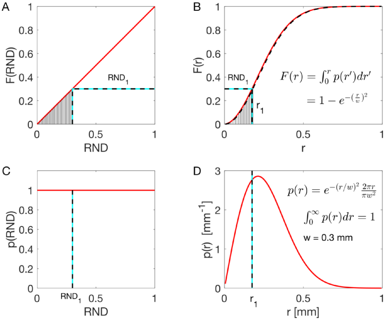
A second example is shown in Fig. 3, illustrating the sampling of a 2D Gaussian beam with a 1/e radius of w. This example is useful for launching a photon into tissue using a collimated Gaussian beam. The goal is to sample the distribution for radial position (r) of photon in the 2D Gaussian beam. Therefore, the rings of integration ( ) must be included and the probability properly normalized: . The integral of p(r) is F(r) = . Solving for a particular using a particular ,
| (5) |
Fig. 3.
Monte Carlo sampling to specify the radial position (r) for launching a photon, such that a population of launched photons would mimic a collimated Gaussian beam with a 1/e radius of w = 3 mm.
This sampling method to specify the launch position for each photon can be applied to a variety of beam shapes amenable to Eq. (2). For beams not amenable to Eq. (2), a lookup table can be used, analogous to the bucket of marbles.
3. Monte Carlo program
This section discusses the basis elements of a MC simulation. The program has three input files: (1) a tissue volume, which specifies the 3D distribution of tissue types (epidermis, dermis, blood, etc.), (2) a list specifying the optical properties of each tissue type (absorption coefficient, scattering coefficient, etc.), (3) a list of run parameters (number of photons to launch, voxel sizes, beam size, etc.) that control the simulation.
3.1. Tissue volume
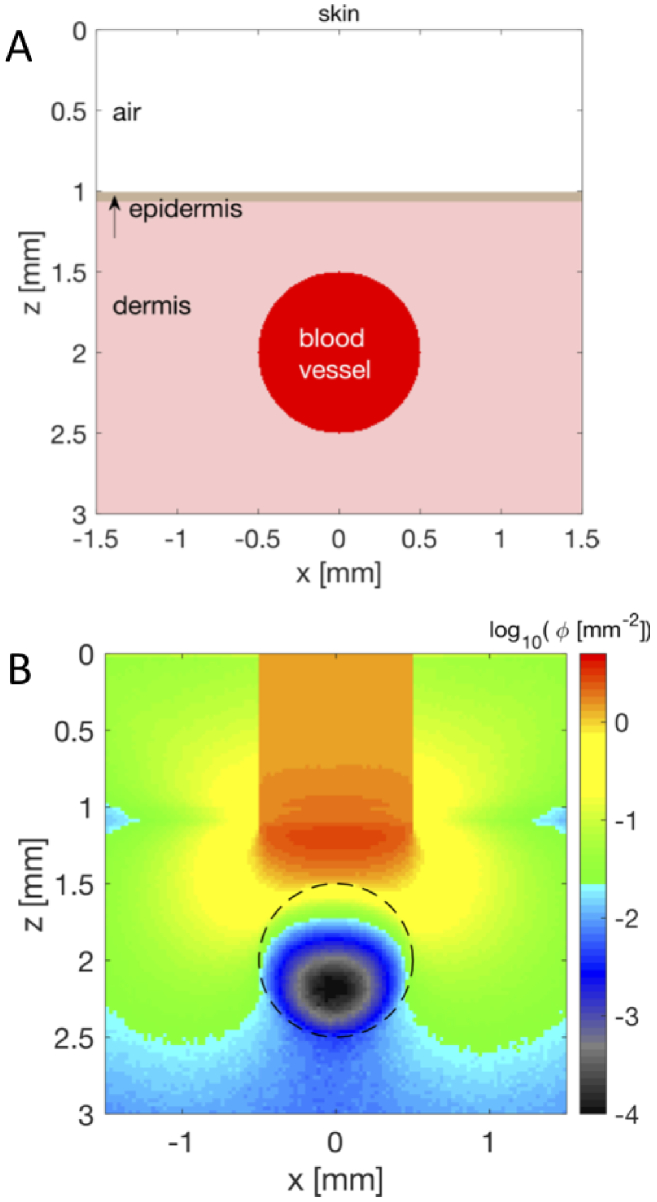
Consider a tissue volume modeled as a cubic array, T(x,y,z), where each voxel is assigned an integer value that specifies a particular tissue type. A complex tissue, such as skin with its several layers (epidermis, papillary dermis, vascular plexus, reticular dermis) along with an embedded tumor and a large blood vessel would have 6 tissue types. The T(x,y,z) voxels would be filled with integers between 1 to 6 to create the tissue structure. The following example shows MATLAB code for generating a two-layer skin tissue (epidermis, dermis) with a 200- m-dia. blood vessel (as shown in Fig. 4). There is specular reflectance of the incident beam at the air/tissue interface ( = 0.0278, ). There is also total internal reflectance when photons strike the air/tissue boundary obliquely as they attempt to escape the tissue ( 0.53).
Fig. 4.
Example of skin tissue with a large blood vessel. The air/skin interface is at z = 1 mm. (A) Tissue structure showing T(z,x)@y=0. There is a 100- m-thick epidermis and a 1-mm-dia. blood vessel centered at 1 mm below the skin surface. (B) Relative fluence, [ ] in response to a 1-mm-diameter 500-nm-wavelength beam of light.
There are a variety of ways to generate a tissue volume T(x,y,z) for input to a MC simulation, this is just one example.
Ny=400; Nx=Ny; Nz=Ny;
dx = 0.010; % mm, 10-um bin size.
dz = dx;
x = ([1:Nx]′–Nx/2)*dx;
z = [1:Nz]′*dx;
T = double(zeros(Nx,Ny,Nz)); % number of voxels in tissue cube
T = T + 4;  % fill background with skin (4 = dermis)
zsurf = 1;  % position of air/skin surface
for iz=1:Nz % for every depth z(iz)
    % air
    if iz<=round(zsurf/dz) % dz = voxel size
        T(:,:,iz) = 1; % 1 = air
    end
    % epidermis (100 um thick)
    if iz>round(zsurf/dz) & iz<=round((zsurf+0.100)/dz)
        T(:,:,iz) = 5; % 5 = epidermis
    end
    % blood vessel @ xc, zc, radius, oriented along y axis
    xc = 0;       % [mm], center of blood vessel
    zc = Nz/2*dz; % [mm], center of blood vessel
    vesselradius  = 0.5; % blood vessel radius [mm]
    for ix=1:Nx
           xd = x(ix) - xc;    % vessel, x distance from vessel center
           zd = z(iz) - zc;    % vessel, z distance from vessel center
           r = sqrt(xd^2 + zd^2);  % r from vessel center
           if (r<=vesselradius)    % if r is within vessel
               T(ix,:,iz) = 3;   % 3 = blood. Extend pattern over all y.
           end
    end %ix
end % iz
3.2. Tissue optical properties
For each tissue type, the optical properties can be generated as a function of wavelength by specifying tissue parameters:
-
1.
B = blood volume fraction (B=1 indicates blood at 150 g/l hemoglobin, or 2.3 mM)
-
2.
S = oxygen saturation of hemoglobin in mixed arteriovenous vasculature
-
3.
W = water content as volume fraction
-
4.
M = melanosome volume fraction (eg., M 0.07 for tanned Caucasian)
-
5.
F = volume fraction of fat
-
6.
= scattering strength ( at reference wavelength, eg., = 500 nm)
-
7.
= fraction of Rayleigh scatter at
-
8.
= fraction of Mie scatter at ( )
-
9.
= scattering power for Mie scatter
-
10.
= anisotropy of scatter ( , is polar angle of photon deflection)
The above tissue parameters are used to calculate the optical properties for a tissue type:
| (6) |
The parameter is the absorption coefficient. The parameter is the reduced scattering coefficient and is used since the literature on tissue optical properties has routinely measured and reported . However, MC simulations use . Alternatively, it is common to use , which works well in the visible wavelength range. The value of anisotropy is sparsely specified in the literature for various tissues, and a value of = 0.90 is commonly used. However, does vary with wavelength and tissue type, and is a parameter deserving more study.
A two-term scattering function can allow separate control of the forward and backward contributions to the overall scattering function [9]. The forward component dominates the penetration of light into a tissue and subsequently the diffuse reflectance due to multiply scattered photons. The backward component dominates the early scatter, perhaps the first 10 scattering events, and the subdiffuse reflectance for the superficial layer of a tissue. The average optical scattering of a tissue may be described by a Plum and Pudding model [10], in which a nucleus (plum) sits within a background of sub-micron scattering structures (pudding).
To illustrate how to use the above tissue parameters, the following excerpt from a MATLAB program makeTissueList.m shows the calculation for epidermis, having requested the optical properties for = 460 nm. A matrix of absorption spectra, MU(nmLIB,1:5) has been loaded, in which 5 columns specify the absorption coefficient of 5 tissue parameters versus wavelength (nmLIB = 300-1000 nm): for oxygenated hemoglobin in blood, for deoxygenated hemoglobin in blood, for water, for the interior of a cutaneous melanosome, for fat. Interpolation yields 5 values for these 5 parameters at a requested wavelength. In this excerpt, a blood-free epidermis with a skin type II is specified. The oxygen saturation S is ignored because there is no blood.
nm = 460; % requested wavelength
MU2 = interp1(nmLIB,MU,nm); % horizontal vector
j=5;  % pointer to tissue type
tissue(j).name  = ′epidermis′;
B = 0; % blood volume fraction
S = 0; % saturation of hemoglobin
W = 0.75; % water volume fraction
M = 0.03; % melanosome volume fraction
F = 0; % fat volume fraction
a = 2; % mm^-1, scattering strength = reduced scattering coeff. at lambda_ref=500nm
fray  = 0.0; % fraction of reduced scattering at 500nm due to Rayleigh scattering
% 1-fray = fraction of reduced scattering at 500nm due to Mie scattering
bmie  = 1.0; % Mie scattering power
g1    = 0.90; % anisotropy of scatter
musp  = a*(fray*(nm/500).^-4 + (1-fray)*(nm/500).^-bmie); % reduced scattering
X     = [B*S B*(1-S) W M F]′; % vertical vector
tissue(j).mua = MU2*X;  % matrix multiplication --> absorption coeff.
tissue(j).mus = a/(1-g1); % scattering coeff.
tissue(j).g1  = g1; % anisotropy of scatter
The values of (tissue(j).mua), (tissue(j).mus), and (tissue(j).g1) are then passed to the MC program as part of the input file.
3.3. Launching photons
This section discusses launching photons. Each photon, sometimes called a “photon bundle", is assigned a weight W = 1.0 at launch, and this W will slowly decrease as absorption occurs with every incremental step of the photon (discussed later in the DROP section). A large number of photons ( ) is launched, where the number depends on the output desired. Only a few thousand may be needed to generate total diffuse reflectance ( [dimensionless]). Perhaps may be needed to generate the point spread function ( ). A few million may be needed to generate the 3D fluence distribution ( ). In all cases, launching more photons reduces the variance in output.
A useful exercise is to run a set of MC simulations, each with its random number generator initiated with a unique seed. Consequently, the outputs of each simulation will be unique. Then the variance of the outputs can be calculated, which offers an estimate of the precision of the result.
Launch position, x,y,z
Each photon is launched at some position x,y,z. Consider how to launch photons at the tissue surface (z=0) as a collimated Gaussian beam with a radius . MC sampling specifies the radial position r of each photon that is launched, then the x,y positions are calculated:
| (7) |
Each photon is launched with a “weight" =1. During propagation the photon’s will drop as photon energy is deposited along the photon’s path, which is discussed later (see Drop).
Photon trajectory, ux,uy,uz
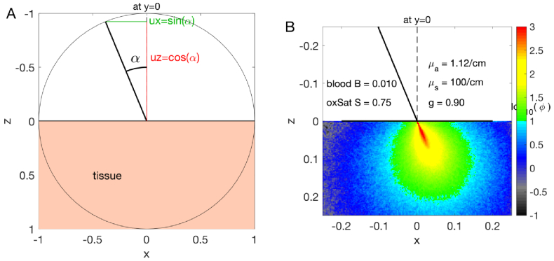
The MC program launches a photon at a position x,y,z with a trajectory vector of unit length specified by ux,uy,uz, where ux is the projection of the vector onto the x-axis, uy projects onto the y-axis, and uz projects onto the z-axis, and therefore . For example, a photon launched at x=0, y=0, z=0 at an angle of 22.5 degrees ( /8 radians) off the normal to the surface and parallel to the x-z plane would have a trajectory specified by ux = cos( /8), uy = 0, uz = cos( /8). Figure 5 illustrates this example.
Fig. 5.
Launching photons (A) A photon is launched at 22.5 degrees ( radians) off the normal to the surface at x=0,y=0, parallel to the x-z plane (i.e., an oblique pencil beam). The trajectory is ux=sin( /8), uy=0, and uz=cos( /8). (B) MC simulation shows the launched photons penetrating a soft tissue (wavelength = 500 nm, = 0.112 , = 100 , =0.90, for the case of 1% blood volume fraction (B) and 75% oxygen saturation of hemoglobin in the mixed arterio-venous vasculature.)
3.4. Propagating photons
A generic flow diagram for propagating photons in a MC simulation is shown in Fig. 6. The following subsections describe the steps in this flow diagram.
Fig. 6.
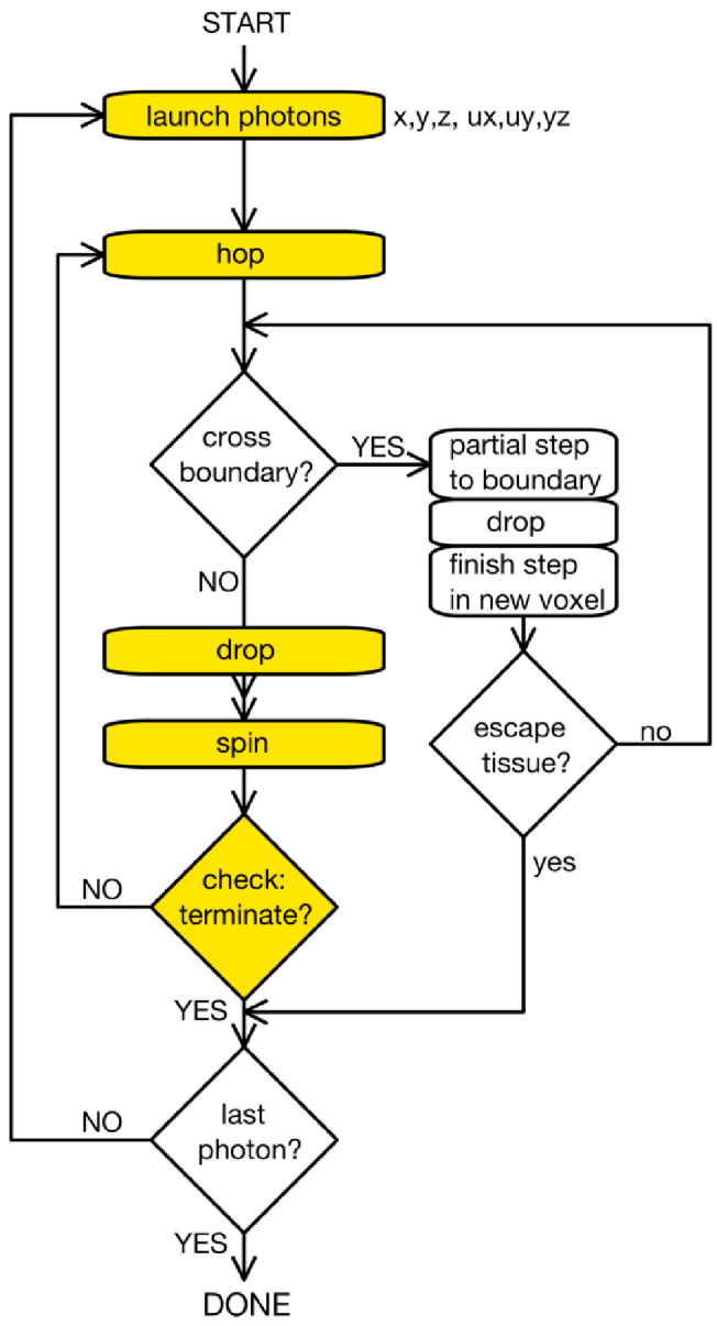
Flow chart for a simple Monte Carlo simulation. Refraction of transmission if photon crosses boundary between voxels, or trajectory change if reflected, based of Fresnel transmission/reflection.
The transport of unpolarized light (a population of photons with randomized orientations of their electric fields) is considered. The basic steps are hop, drop, spin, and check, as in Fig. 6.
Hop
The HOP step samples a step size ( ) for the photon before it encounters its next scattering event,
| (8) |
This step size is weighted exponentially, and is sampled as illustrated in Fig. 2. Alternatively, the program mcml.c uses the expression,
| (9) |
where . The step is between “interactions", at which a fraction of the photon weight, , survives and a fraction is absorbed. The two methods give the same results when many photons are launched. However, Eq. (8) is perhaps more appropriate when considering the first few scattering events in a tissue, such as the study of photon scatter in a superficial epithelium. This tutorial uses the first method (Eq. (8)).
The position of a photon is updated by the step size , where the movement in each x,y,z direction is scaled by the trajectory vectors :
| (10) |
where , , are the projections of the photon trajectory onto the x, y, and z axes.
Crossed a boundary?
The voxel in which the photon resides is specified by the ix, iy, iz pointers to the voxel, which are obtained by taking the integer value of each x,y,z position. For example in MATLAB notation, the function where is the voxel size converts to such that . In other words it does not “round up" to when is closer to . In C code, accomplishes the same function. Similarly, iy and iz are determined. If the voxel pointers before and after taking step are the same, the photon is still in the same voxel. But if they differ, then the photon is crossing a voxel boundary.
If the photon is attempting to cross a boundary, then the step must be divided into a step to the voxel boundary, drop some photon weight in the current voxel (see Drop below), then take the remainder of the step, , in the next voxel, governed by the optical properties of that voxel. The photon step is split based on its dimensionless value where subscript 1 indicates the current voxel. The step along to the voxel boundary at is with a dimensionless value , where is the scattering within the current voxel. Similarly, the steps along y and z are calculated. The minimum along the x,y,z directions becomes the step size to the boundary. The photon hops to the boundary with step , and drops some weight in the current voxel (see Drop section). The position of the photon is advanced by a negligible amount (eg., mm) to cross the boundary. Then it continues with its remaining weight in the new voxel with a step based on the remaining dimensionless step, , as in the following equations,
| (11) |
Transmit or reflect?
Not explicitly shown in Fig. 6 is a decision on whether to reflect off the boundary being crossed or to transmit across the boundary. This decision occurs in the cross boundary step of Fig. 6. If the refractive indices of the current and next voxel, and , are different, then a subroutine is called, which is based on Fresnel reflectance, where r is the Fresnel reflectance of the boundary, and are the refractive indices of the current and new voxel, is the cosine of the angle of incidence onto the boundary, and is the cosine of the angle of transmittance. The subroutine returns and . A random number is then generated, and if then the photon reflects off the boundary. Otherwise, it transmits into the new voxel at the angle . This handling of the boundary works well when regions of different refractive indices are aligned with the xy, xz, or yz planes. However, a tissue structure with curved regions of different refractive indices requires guidance by the curved surface to refract correctly. An example of such guidance is demonstrated in the MC program reported by Tran and Jacques [11].
Escaping?
When crossing a boundary, a transmitted photon may be crossing a surface boundary (eg., tissue/air) and escaping the tissue. In this case, after the partial step to the boundary and the calculation of the escaping trajectory angle, the photon weight can be assigned to increment an element of an array of escaping flux J(x,y,z) at some x,y,z position, at some angles of escape J( ), or a combined J(x,y,z, ). If the photon is not escaping, it returns to the step “Cross boundary?" and continues propagating.
Drop
The DROP step deposits some of the photon weight ( ) into an array element associated with the current voxel, , then decreases the surviving weight of the photon,
| (12) |
where is the step length taken within the current voxel, is the absorption coefficient of the current voxel, and is the current weight of the photon. Each photon contributes to the accumulation of the spatial distribution of deposited photon weight, A(x,y,z) [dimensionless], which records the fraction of the total energy of all delivered photons that was deposited in each x,y,z voxel. This A(x,y,z) is later converted to relative fluence rate (see OUTPUT module).
Spin
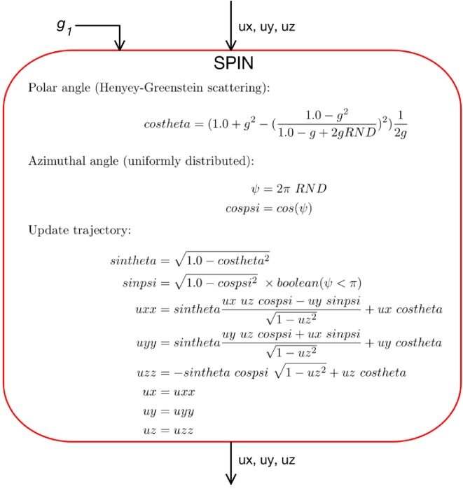
The SPIN step changes the trajectory of the photon based on a chosen scattering function, i.e., it updates the parameters ux, uy, uz. Figure 7 shows the calculations within the SPIN module. Each use of RND is a freshly generated random number.
Fig. 7.
The SPIN module changes the trajectory of the photon, specified by (ux,uy,uz).
This example uses the Henyey-Green scattering function, controlled by the anisotropy for the tissue in the current voxel. First, the polar deflection angle, , is sampled, yielding the parameter costheta. Second, the azimuthal angle of scatter, , is sampled, yielding cospsi, as if it were randomly distributed between 0 and , since the scattering structures are randomly oriented. This is the usual assumption but in some cases, for example striated muscle, there is an orientation to the scattering structures and the azimuthal angle may have to be sampled appropriately. Third, the costheta and cospsi along with the current trajectory (ux,uy,uz) are used to create a new trajectory (uxx,uyy,uzz), which is then assigned to ux,uy,uz. Hence, the photon trajectory has been adjusted by a single scattering event.
Check
A final step in this iterative hop, drop, spin, check process is the Check module to properly terminate a photon. Since the photon weight W continually decreases as the photon propagates, at some point the W is so low that continuing to propagate the photon adds little to the final solution. However, one cannot simply terminate the photon because the residual W will be lost, violating conservation of energy and resulting in an erroneous result. So the photon is statistically terminated using the so-called “Roulette Method". When W drops below a threshold value, a random number (RND) is generated, and if RND is less than a value chance (0 < chance < 1), then W is increased by . Otherwise, the photon is terminated.
chance = 0.10
threshold = 0.001
if W <= threshold
     if RND<chance, W = W/chance
     else W=0 (kill photon)
else do_nothing (photon continues)
The choice of threshold = 0.001 means that 99.9% of a photon’s weight has been deposited before considering to extend the photon’s life by increasing its weight. The choice of chance = 0.1 means that the photon terminates 90% of the time and 10% of the time the photon’s W is increased 10-fold to allow the photon to continue propagating. Statistically this procedure conserves energy (Escape + Absorption = 1). The conservation of energy is the key reason for the roulette method. When a photon’s lifetime is extended, it may escape as reflectance or transmission, or it may be absorbed. The expanded spatial extent of photon movement afforded by this lifetime extension of 0.01% of the photons balances the loss of photon movement for 99.99% of the photons.
Once a photon is terminated, another photon with a fresh W = 1.0 is launched. Photons are launched until the requested number of photons is reached, which terminates the launching of photons. The simulation is now complete, and the program then proceeds to the OUTPUT module to generate a report of results.
3.5. Output
After photons have been launched, a final step of scaling is needed to generate the output for the user.
3.5.1. Absorbed photon fraction, A(x,y,z)
The absorbed fraction A(x,y,z) holds the total weight deposited by all the photons in the voxel at x,y,z. This weight is then normalized by the number of photons launched and by the volume of the voxel to yield a density of photon deposition, . For an input of 1 J, A indicates . For an input of 1 W, A indicates .
3.5.2. Photon energy concentration or fluence, (x,y,z)
The Monte Carlo simulation has recorded and scaled A(x,y,z) as , which is related to the fluence at that voxel by the absorption coefficient of that voxel,
| (13) |
If the incidence is 1 J of energy, as in a pulsed laser, the fluence has units of [ ], which might be called the radiant exposure experienced by the voxel. If the incidence is 1 W of power, the fluence rate is expressed as [ ], which might be called the irradiance experienced by the voxel. The fluence rate in [ ] is proportional to the instantaneous energy density in the voxel, : , where is the speed of light in the medium ( . is speed in vacuo, is refractive index).
3.5.3. Escaping flux, J(x,y,z, )
The light that escapes the tissue was recorded as photon weight W escaping at some x,y,z position and angles , J(x,y,z, ) [dimensionless weight]. To illustrate, consider the total escape at all angles from one voxel at the front surface of a tissue slab where light was delivered, J(x,y) at z=0. This escaping weight is then normalized by the number of photons launched and the surface area ( ) of the voxel from which the photons escaped: with units of [ ], which is a flux density. Such escape from the irradiated surface may be called local reflectance, , and the total diffuse reflectance is . Escape from the rear surface of a tissue slab may be called local transmittance and the total diffuse transmission similarly calculated. For tissue geometries other than slabs, total reflectance and transmittance are not always the best descriptors, and the local flux density of escape may be more appropriate.
It is also possible to record the escaping photon weight as a function of the polar ( ) and azimuthal ( ) angles of escape into the medium outside the tissue. Usually, the azimuthal variation of escape is uniform since scatters are randomly oriented, so only the polar variation is recorded. For example, record where is divided into increments from 0 to , i.e., reflectance orthogonal to tissue surface ( ) to the extreme of broad scatter ( ). Then, the cumulative sum of from 0 up to some yields the escape that would be collected by the numerical aperture of a detector centered on the z-axis at x,y=0,0 ( ). Interpolation of this cumulative sum can yield the collection of any particular detector (eg., optical fiber, camera).
In summary, the MC simulation can yield a deposition, a fluence, or an escaping flux expressed as a fraction of the delivered power [W] or energy [J]. Considering effects of light on the tissue, the deposited energy, per J delivered = , causes heating or photochemistry. Considering diagnostics, the escaping flux, W per W delivered = reflectance (not including specular reflectance), or escaping flux density, per W delivered = local reflectance, provide information about the tissue. Deposited energy within the tissue will affect the escaping flux, allowing the diagnostic detection of local absorbing structures like a blood vessel or tumor.
3.6. Nuances in MC code
There are nuances when setting up a MC simulation. For example, the lateral boundaries at x and y may allow photons to escape the simulation volume and never return, which drops the fluence near these boundaries. Setting the boundaries to act like a mirror can prevent such loss, but now there are virtual images of the source and tissue structure appearing outside the volume and too much light may return from the boundary. Either a compromise between these two boundary conditions is needed, or photons are allowed to propagate outside the simulation volume and later return into the volume. Another nuance is to be sure that the boundaries between different tissue types are aligned with the bins of the simulation. For example, if the boundary between two tissue types occurs within a voxel, rather than at the front or rear surface of the voxel, then photons in that voxel will sometimes act as if in the first tissue type and sometimes as if in the second tissue type, resulting in odd results at that voxel. The possible nuances depend on the particular implementation of a MC simulation.
3.7. Polarized light and coherence
The character of a photon can be characterized by the orientation and phase of its oscillating electric field. A population of photons can be described by a polarization state, the Stokes vector = [I Q U V]. Ramella-Roman et al. [12] describe a MC simulation of polarized light propagation, which was recently implemented in a GPU-accelerated simulation [13].
The propagation of coherence by a MC simulation tracks the orientation and phase of a photon as it propagates. At a detector or region of interest, multiple photons add via vector addition to yield the net intensity, orientation, and phase. Fischer et al. [14] describe a MC simulation that predicts the spatial coherence of light propagation. Shen et al. [15] describe propagation of coherence in random medium. Sawicki et al. [16] describe a MC simulation of coherent backscatter from a tissue.
4. Example uses
4.1. How does skin architecture affect skin color?
The light reflected from the skin over the 380-720 nm range of wavelengths yields the perceived color of the skin. A set of Monte Carlo simulations can specify a diffuse reflectance spectrum over this range of wavelengths ( ), which can be converted into a triplet of red, green, and blue values (R,G,B) which combine to yield a perceived color.
The CIE standard observer functions, , multiply the reflectance spectrum, the illumination spectrum ( ), and the daylight spectrum ( ), followed by integration to yield an X,Y,Z triplet of values.
| (14) |
The next step uses a transformation matrix M to transform the triplet X,Y,Z into the triplet R,G,B (an XYZ sRGB transformation). This M is based on the daylight illumination ( , 6500 color temperature).
| (15) |
where superscript indicates the transpose to a vertical vector, and M is the transformation matrix,
| (16) |
The resulting R,G,B triplet combines to yield the skin color. The wavelength dependence of the and the M matrix cancel each other. If = 1.0 and R = 1.0 for all wavelengths, the R,G,B triplet yields a white color on a computer screen. If a particular is used in Eq. (14), then the displayed color will properly portray the perceived color under that particular illumination.
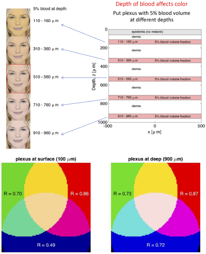
Consider a four-layer skin architecture: (1) a pigmented epidermis with low melanin to allow better display of the skin color, (2) a superficial papillary dermal layer with low blood content (just thin capillaries), (3) a 50- m-thick vascular plexus with 5% blood content serving as the reservoir for supplying the capillaries, and (4) a deeper reticular dermis with a few larger blood vessels feeding/draining the vascular plexus. Figure 8 shows the skin model and the resulting colors. When the plexus is close to the skin surface, the skin color is slightly orange. As the plexus is moved further from the surface, the skin turns slightly pink. Why?
Fig. 8.
As a 50- m-thick vascular plexus with 5% blood content is moved further from the skin surface, the skin color changes from slightly orange to slightly pink. Above the plexus, the dermis is relatively blood free with only thin capillaries circulating red blood cells. Blue light is partially reflected from this superficial layer before it can reach the blood in the plexus and be absorbed, hence blue reflectance increases. This simple model only approximates true skin structure to illustrate the effect.
In the homogeneous skin model, the red, green, and blue light pass through a uniformly blood-perfused skin. The absorption of light by blood scales as blue > green > red, yielding an R,G,B triplet of [0.86 0.70 0.49], which is slightly orange. In the layered skin model, the red light and green light penetrate into the reticular dermis, then diffuse back out to escape at the surface, hence red and green light pass through the vascular plexus twice. Blue light, however, has difficulty penetrating into the plexus because it is strongly scattered by the relatively blood-free superficial layer. Consequently, blue light partially avoids absorption by blood and more blue is reflected. The R,G,B triplet is [0.87 0.73 0.72], which is slightly pink.
The same effect of architecture can be seen in pink gums, blue eyes, and blue monkey butts. The latter two examples feature a superficial collagenous layer overlaying a layer of melanin pigment. Blue light scatters and red and green penetrate to the melanin and are absorbed. In summary, tissue architecture affects the perceived color of a tissue.
4.2. Exposure time for photobiomodulation of the knee?
Photobiomodulation therapy (PBMT) is a phototherapy often using deep red light to elicit a biological effect on a tissue such as decreasing inflammation after tissue injury. The mechanism of PBMT is still a subject of investigation and several possible mechanisms are considered [17]. One mechanism involves interaction of treatment light with the cytochrome C pigment in the inner walls of the mitochondria, thereby affecting electron transport.
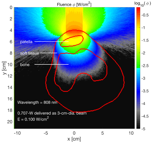
A typical dose of light for PBMT is 1 . Figure 9 shows the irradiation of a knee with 0.707-W collimated beam delivered uniformly over a 3-cm-dia. spot, which equals 0.100 irradiance. This irradiance is commonly used in phototherapy to avoid overheating by allowing blood flow to cool the tissue. The figure indicates that fluence rate in the soft tissue between the patella and bone is about 0.01 . Delivery of the beam for two minutes yields (0.01 )(60 s/min)(2 min) = 1.2 within the soft tissue. Therefore, a two-minute treatment may be approximately sufficient for treatment.
Fig. 9.
Photobiomodulation therapy (PBMT) of the knee. The delivery of 0.707 W of treatment light at 808-nm wavelength over a 3-cm-dia. spot yields an irradiance E = 0.100 , which penetrates into the knee to yield about 0.01 fluence in the soft tissue between the patella and bone.
4.3. Will a pulsed laser treatment reach the bulb of a hair follicle?
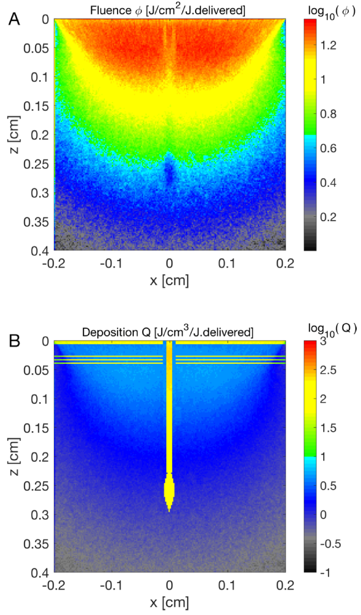
Laser treatment sometimes employs thermal coagulation of tissue to achieve a therapeutic effect. A popular example is the use of a pulsed laser to cause thermal damage to the bulb of a hair follicle for the purpose of hair removal. Figure 10 illustrates the penetration of a 0.4-cm-dia. 1024-nm infrared pulsed laser down to the bulb. The focus does not reach the bulb due to light scattering by the tissue, however, diffusion allows light to reach the bulb. The energy deposition in the bulb reaches about 100 per J delivered. Therefore, a 1.9-J 10-ms laser pulse (15 exposure at skin surface) increases the C skin temperature to (1.9 J)(100 /J)/(4 C. ) + C = C, which is sufficient to thermally damage the bulb.
Fig. 10.
(A) Penetration of a pulsed 1024-nm-wavelength 0.4-cm-dia. laser beam focused to the bulb of a hair follicle at a depth of 0.3 cm in the skin. The beam loses its focus within 1 cm and only diffuse light reaches the bulb. The depression of fluence along z at x=0 is due to absorption by the melanin pigment in the epithelium of the hair shaft. (B) The energy deposition in the bulb is sufficient to achieve thermal damage. The bulb has a 50% volume fraction of cutaneous melanosomes.
5. Conclusion
This tutorial has briefly discussed the typical design of a Monte Carlo (MC) simulation of light transport for the purposes of diagnostics and dosimetry during biomedical applications of light. There are now a number of MC simulations available on the internet for biomedical, oceanic, atmospheric, and astrophysical applications. The tutorials for using specific MC programs can instruct on how to use these programs.
Acknowledgments
The author’s adventure with Monte Carlo simulations was shared with Scott Prahl, Marleen Keijzer, Lihong Wang, Jessica Ramella-Roman, Ting Li, Yinchu Chen, and Anh Phong Tran, who all contributed to development of mcml.c and mcxyz.c.
Disclosures
The author declares no conflicts of interest.
Data availability
No data were generated or analyzed in the presented research.
References
- 1.Metropolis N., “The beginning of the Monte Carlo method,” Los Alamos Science, Special issue, 125–1330 (1987). [Google Scholar]
- 2.Wang L., Jacques S. L., Zheng L., “MCML - Monte Carlo modeling of light transport in multi-layered tissues,” Computer Methods and Programs in Biomedicine 47(2), 131–146 (1995). 10.1016/0169-2607(95)01640-F [DOI] [PubMed] [Google Scholar]
- 3.Marti D., Aasbjerg R. N., Anersen P. E., Hansen A. K., “MCmatlab: an open-source, user-friendly, MATLAB-integrated three-dimensional Monte Carlo light transport solver with heat diffusion and tissue damage,” J. Biomed. Opt. 23(12), 1 (2018). 10.1117/1.JBO.23.12.121622 [DOI] [PubMed] [Google Scholar]
- 4.Fang Q., Boas D. A., “Monte Carlo simulation of photon migration in 3D turbid media accelerated by graphics processing units,” Opt. Express 17(22), 20178 (2009). 10.1364/OE.17.020178 [DOI] [PMC free article] [PubMed] [Google Scholar]
- 5.“Virtual Photonics Technology Initiative,” (2022) https://virtualphotonics.org.
- 6.“MCX, Monte Carlo eXtreme, a GPU-accelerated photon transport simulator,” (2022), http://mcx.space.
- 7.“Cloud based Monte Carlo tool for photon transport,” (2022), http://www.lighttransport.net.
- 8.Jönsson J., Berrocal E., “Multi-Scattering software: part I: online accelerated Monte Carlo simulation of light transport through scattering media,” Opt. Express 28(25), 37612–37638 (2020). 10.1364/OE.404005 [DOI] [PubMed] [Google Scholar]
- 9.Jacques S. L., McCormick N. J., “Two-term scattering phase function for photon transport to model subdiffuse reflectance in superficial tissues,” Biomed. Opt. Express, in press (2022). [DOI] [PMC free article] [PubMed]
- 10.Xu M., “Plum pudding random medium model of biological tissue toward remote microscopy from spectroscopic light scattering,” Biomed. Opt. Express 8(6), 2879 (2017). 10.1364/BOE.8.002879 [DOI] [PMC free article] [PubMed] [Google Scholar]
- 11.Tran A. P., Jacques S. L., “Modeling voxel-based Monte Carlo light transport with curved and oblique boundary surfaces,” J. Biomed. Opt. 25(02), 1 (2020). 10.1117/1.JBO.25.2.025001 [DOI] [PMC free article] [PubMed] [Google Scholar]
- 12.Ramella-Roman J. C., Prahl S. A., Jacques S. L., “Three Monte Carlo programs of polarized light transport into scattering media: part I,” Opt. Express 13(12), 4420–4438 (2005). 10.1364/OPEX.13.004420 [DOI] [PubMed] [Google Scholar]
- 13.Yan S., Jacques S. L., Ramella-Roman J. C., Fang Q., “Graphics-processing-unit-accelerated Monte Carlo simulation of polarized light in complex three-dimensional media,” J. Biomed. Opt. 27(08), 083015 (2022). 10.1117/1.JBO.27.8.083015 [DOI] [PMC free article] [PubMed] [Google Scholar]
- 14.Fischer D. G., Prahl S. A., Duncan D. D., “Monte Carlo modeling of spatial coherence: free-space diffraction,” J. Opt. Soc. Am. A 25(10), 2571–2581 (2008). 10.1364/JOSAA.25.002571 [DOI] [PMC free article] [PubMed] [Google Scholar]
- 15.Shen Z., Sukhov S., Dogariu A., “Monte Carlo method to model optical coherence propagation in random media,” J. Opt. Soc. Am. A 34(12), 2189 (2017). 10.1364/JOSAA.34.002189 [DOI] [PubMed] [Google Scholar]
- 16.Sawicki J., Kastor N., Xu M., “Electric field Monte Carlo simulation of coherent backscattering of polarized light by a turbid medium containing Mie scatterers,” Opt. Express 16(8), 5728 (2008). 10.1364/OE.16.005728 [DOI] [PubMed] [Google Scholar]
- 17.Hambin M. R., Farraresi C., Huang Y., Freitas de Freitas L., Carroll J. D., Low-level Light Therapy: Photobiomodulation (SPIE Press, 2018). [Google Scholar]
Associated Data
This section collects any data citations, data availability statements, or supplementary materials included in this article.
Data Availability Statement
No data were generated or analyzed in the presented research.


