Abstract
Surface defects are a common issue that affects product quality in the industrial manufacturing process. Many companies put a lot of effort into developing automated inspection systems to handle this issue. In this work, we propose a novel deep learning–based surface defect inspection system called the forceful steel defect detector (FDD), especially for steel surface defect detection. Our model adopts the state-of-the-art cascade R-CNN as the baseline architecture and improves it with the deformable convolution and the deformable RoI pooling to adapt to the geometric shape of defects. Besides, our model adopts the guided anchoring region proposal to generate bounding boxes with higher accuracies. Moreover, to enrich the point of view of input images, we propose the random scaling and the ultimate scaling techniques in the training and inference process, respectively. The experimental studies on the Severstal steel dataset, NEU steel dataset, and DAGM dataset demonstrate that our proposed model effectively improved the detection accuracy in terms of the average recall (AR) and the mean average precision (mAP) compared to state-of-the-art defect detection methods. We expect our innovation to accelerate the automation of industrial manufacturing process by increasing the productivity and by sustaining high product qualities.
Keywords: Steel defect detection, Deformable convolution, Deformable RoI pooling, Feature pyramid network, Guided anchoring, Region proposal network
Introduction
Industrial surface defect detection is a critical step to ensure product quality. In order to relieve inspectors of laborious work and improve the consistency of inspection, much effort has been dedicated to automating the inspection process using computer vision approaches over the past decades [1–3]. However, conventional computer vision approaches have been limited in their effectiveness due to varying illumination conditions and similarities between the surface textures and defects. Recently, Industry 4.0 has become a popular notion to achieve the goal of intelligent manufacturing [4], wherein manufacturing technologies will shift from automatic to “smart manufacturing.” The main goal is to achieve the best performance and highest efficiency in the production process.
Nowadays, with the rising popularity of deep learning techniques for visual recognition, deep learning–based defect detection has been extensively applied to surface defect inspection systems [5–12].
There are three categories of deep learning–based defect inspection systems, which are based on classification, object detection, and object segmentation. Classification-based defect inspection systems [13–21] categorize an input image as defect or non-defect and calculate the class probability using stacks of convolutional neural networks. This approach is simple, but it cannot localize defects. To localize various defects in an input image, object detection–based defect inspection systems called defect detectors were developed [5, 7, 11, 22, 23]. Based on this approach, defect locations can be predicted as bounding boxes, along with defect class labels and confidence scores. There are two types of object detection–based defect detectors [24]. The first is a one-stage method [12, 25–31], which simultaneously detects and localizes defects. This method achieves a fast inference speed at the cost of lower precision. The second is a two-stage method [7, 12, 32–34]. It first generates region proposals for possible defect locations; then, the region proposals are passed along a pipeline for defect classification and bounding-box regression. Such a method is slower, but it reaches higher detection accuracy. Besides, segmentation-based defect inspection systems [6, 12, 35] were also developed, which identify the shape of defects by using a pixel-wise mask. This technique provides a far more granular understanding of the defects in an image. However, the inference speed is much slower than that of object detection–based methods because it requires pixel-level defect and non-defect predictions. According to the above discussion, object detection–based defect detection offers a better trade-off between accuracy and complexity; hence, it is more suitable for industrial applications.
In this paper, we propose a novel object detection–based defect detection system, called the “forceful defect detector” (FDD). Moreover, the proposed FDD begins with enriching the point-of-view of input images. We propose a data preprocessing pipeline which involves a random scaling scheme [36] in the training stage and the ultimate scaling technique in the inference stage. Next, we adopted Cascade RCNN [32] as the object detection network and enhanced it with deformable operation and guided anchoring region proposal network (GA-RPN) [37]. Finally, our experimental studies show that the proposed method achieves higher defect detection accuracy on famous defect datasets [7, 12, 38] compared to existing models and maintains a processing speed which meets the standard for steel surface inspection systems [39, 40]. The remaining of this paper is organized as follows. Section 2 presents the related works on defect detection. In Section 3, we elaborate on the proposed FDD in detail. In Section 4, the effectiveness of the proposed method is demonstrated through experimental studies. Section 5 concludes the paper.
Related works
Object detection–based defect inspection systems locate the defective area in an image by generating bounding boxes. State-of-the-art one-stage object detectors are you only look once (YOLO) family and transformer networks. For example, YOLOv4 [26] improves on the classical YOLOv3 [41] by selecting suitable components to enhance the detection performance, such as Mosaic data augmentation, CSPDarknet53 [42] with the spatial pyramid pooling (SPP) block [43] as the backbone, PANet [44] path-aggregation neck, followed by the YOLOv3 anchor-based prediction head. Recently, YOLOv5 [27] improved the inference speed of YOLOv4, and YOLOX [28] incorporated the free anchor concept to improve YOLOv3’s prediction head accuracy.
Other one-stage object detection methods also improved YOLOv3 by incorporating new elements. For example, CP-YOLOv3-dense [31] combined YOLOv3 with Dense Convolutional Network (DenseNet) [45] to detect surface defects of steel strips. The model can receive multi-layer convolutional features output by the densely connected blocks before making predictions, thereby enhancing feature reuse and feature fusion. A Lightweight End-to-End Network for Surface Defect Detection (LSSDN) [46] was proposed to identify the defects on a textured surface. This lightweight network comprises three major parts: The stem part quickly reduces the size of the feature maps, the trunk part is composed of three stages for multi-level feature extraction, and finally, YOLOv3 serves as the detection part.
Besides, RetinaNet [47] proposed the focal loss to solve the class imbalance problem. RetinaNet with difference channel attention and adaptively spatial feature fusion (DEA_RetinaNet) [30] improved the performance of RetinaNet for steel defect detection. CenterNet with dilated feature enhancement model, center-weight, and CIoU loss (DCC-CenterNet) [29] is a variant of CenterNet [48], which proposed a dilated feature enhancement model (DFEM) to enlarge the receptive field of features; thus, the network can effectively detect the defects of different scales.
In recent years, the transformer [49] has emerged as an effective architecture to explore global correlations among a sequence of inputs. It was successfully applied to image classification [50], semantic segmentation [51, 52], and object detection [25, 53]. The pyramid vision transformer (PVT) [54] combined transformer layers with the feature pyramid network (FPN) [55] to extract features and adopted the RetinaNet [47] as the detection head. The updated version PVTv2 [25] improved PVT by adding three designs: overlapping patch embedding, convolutional feed-forward networks, and linear complexity attention layers.
In contrast to one-stage object detectors, two-stage object detectors can achieve a higher detection accuracy. Among famous two-stage object detectors, Faster R-CNN [56] uses the FPN as a neck between the backbone network and prediction head to enable multi-scale feature extraction. Cascade R-CNN [32] improved upon Faster R-CNN by proposing iterative prediction heads with different IoU thresholds from small to large. This iterative process uses cascade regression as a sampling procedure to provide good samples from one stage to another. On the other hand, DetectoRS [33] improved the FPN structure by proposing the recursive feature pyramid and switchable atrous convolution. This sequentially repeats the FPN process and uses the feedback signal to improve the accuracy of each stage.
For defect detection, the two-stage method defect detection network (DDN) [7] proposed a multi-level feature fusion network (MFN) to integrate lower-level and higher-level features to include more location details of defects. Defect inspection network (DIN) [34] utilized deformable convolution [57], balanced feature pyramid [58], and Fast R-CNN head [59] to accommodate steel defects with arbitrary shapes. Another two-stage model [60] was developed to handle the complicated defect detection task on steel surface datasets, which contain critical problems such as vagueness and tiny defects. Moreover, the inspection model proposed in [22] combined the two-stage method with an attention network to detect defects for solar cell electroluminescence (EL) images, which is a challenging task on the manufacturing side due to the similarity between background and foreground features.
The proposed forceful defect detector
Our proposed defect inspection system, named the forceful defect detector (FDD), consists of a data preprocessing pipeline which involves a random scaling scheme for model training, the baseline detector, the deformable operation, the guided anchoring, and the ultimate scaling scheme for the inference stage. In general, we developed this system based on several reasons. First, to enrich the point-of-view of input images, we propose a data preprocessing pipeline which involves a random scaling scheme [36] in the training stage, randomly resizing the input image while maintaining its original aspect ratio. In the inference stage, we propose the ultimate scaling technique to scale the input image to an optimal size. Second, to ensure high-quality feature extraction, our proposed network begins with a 5-stage feature pyramid network (FPN) [55], each stage involving the state-of-the-art aggregated residual transformation block (ResNext) [61]. Third, instead of the standard convolution [62], the proposed system utilizes the deformable convolution [57] at stages 3 to 5 and deformable region of interest (RoI) pooling, which are more suitable for extracting features from the geometric shape of the defect. Fourth, we replace the general region proposal network (RPN) head with the guided anchoring region proposal network (GA-RPN) [37] to generate more precise bounding boxes. Furthermore, this section will discuss the parts of the system in more detail.
Data preprocessing pipeline
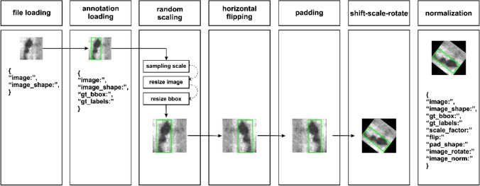
As shown in Fig. 1, steel defects usually have different features, such as various scales, directions, and shapes. To train a detection model robust to these features, we propose a data preprocessing pipeline as shown in Fig. 2. The first two blocks are the standard image loading and annotation. We followed the Pascal VOC format [63] to generate bounding box annotations for the datasets.
Fig. 1.
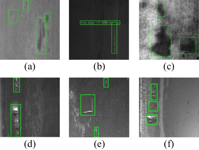
As a result of defect randomness, a and d show varying scales and b and e show varying directions, while c and f show arbitrary shapes
Fig. 2.
The proposed data preprocessing pipeline
The third block in Fig. 2 is our proposed random scaling scheme. Our proposed random scaling method helps to train a more generalized model to detect defects of various scales.
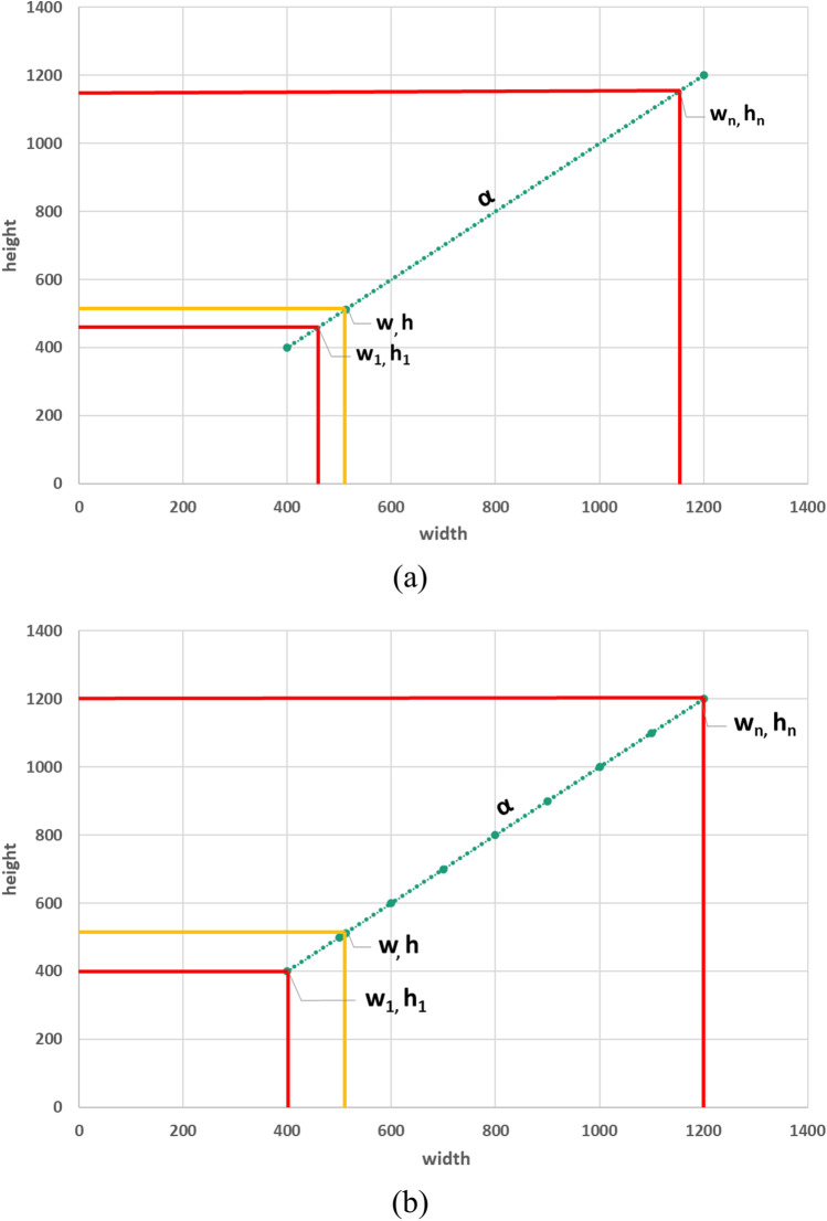
As shown in Fig. 3, image resizing is widely used as one important technique in deep learning–based object detection. There are three existing image resizing methods: uniform scaling [64], progressive resizing [65], and sampling scaling [36]. The uniform scaling method shown in Fig. 3a resizes all the original training images into images of a single size. For object detection, this has often resulted in losing key defect features, because the network only learns the defect feature from one fixed size. It may result in identifying only small defects or large defects and ignores the others. Progressive resizing, on the other hand, scales up the input image into three different sizes. The network is trained with the first size and then fine-tuned with the other two different sizes. It has become a powerful solution to boost the object detection performance [36] and was recently adopted to help screen Covid-19 cases [66]. In contrast, the sampling scaling method as shown in Fig. 3b randomly resizes the input images and the bounding boxes to different sizes in different epochs during the training process. This helps in detecting defects of different sizes. Meanwhile, it avoids the high computational complexity of progressive resizing, caused by using multiple scales for the same input image.
Fig. 3.
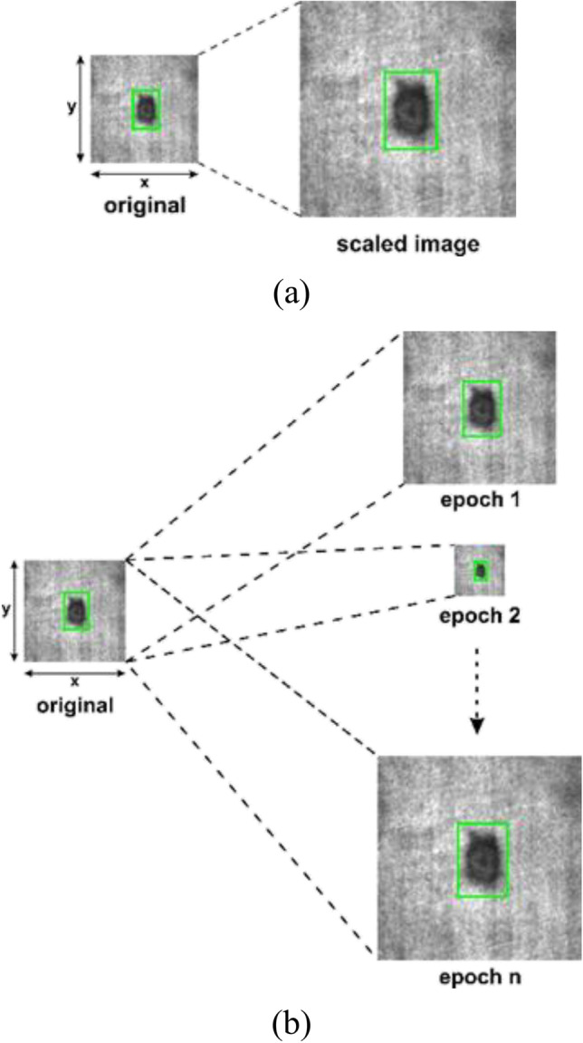
a Uniform scaling; b sampling scaling
Inspired by the idea of sampling scaling, in the third block of Fig. 2, we propose a random scaling scheme, randomly resizing the input image while maintaining its original aspect ratio. For example, Fig. 4a shows that if we have an input image with an aspect ratio , where and are the original width and height of the image, then the new height is randomly chosen from a set of integers as (1), and the new width is determined by (2).
| 1 |
| 2 |
Fig. 4.
The proposed a random scaling for training and b ultimate scaling for inference
Once we have resized the input image, the height and width of the bounding box in the original input image is also resized by the following:
| 3 |
where and are the original height and width of the bounding box, and and are the resized height and width of the bounding box.
The fourth block in Fig. 2 performs horizontal flipping, followed by padding operation in the fifth block. The sixth block is shift-scale-rotate, followed by the last block that normalizes the input image.
The baseline detector
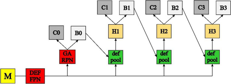
Figure 5 shows our proposed forceful steel defect detector (FDD). We adopt the two-stage detector Cascade R-CNN [32] as our baseline architecture. First, the FPN backbone extracts and combines features of small and large scales, which belong to small and large defects, respectively.
Fig. 5.
The proposed forceful defect detector network, where M is the preprocessing blocks in the training stage and ultimate scaling in the inference stage, DEF-FPN is the backbone feature pyramid network with deformable convolution, GA-RPN is the guided anchoring region proposal network head, def pool is the deformable RoI pooling, H is the R-CNN head, C is the output class label, and B is the output bounding box
Next, the RPN will generate proposals based on the multi-scale feature maps generated by the FPN. An output feature map will show whether a defect is present in the input image at a particular location and its estimated size. This is done by placing a set of “Anchors” on the output feature map of the backbone network. These anchors indicate defects of different sizes and aspect ratios that could be present at this location in the form of bounding boxes.
Prior R-CNN baselines or Faster R-CNN [56] define ROIs as defect proposals with at least 0.5 IoU with the foreground bounding box. On the contrary, cascade R-CNN refines the proposals sequentially based on three IoU thresholds: 0.5, 0.6, and 0.7, respectively, and generates bounding boxes and defect classes based on these refinements.
In Cascade R-CNN, the three successive R-CNN modules, as shown in Fig. 5, refine the proposals sequentially with three different IoU thresholds: 0.5, 0.6, and 0.7, respectively, and generate the final predicted bounding boxes and defect classes.
Furthermore, we improved the baseline Cascade R-CNN by the following components: First, we process the original input image by module “M,” which represents the preprocessing blocks in Fig. 1 during the training stage and represents the ultimate scaling scheme during the inference stage. The ultimate scaling scheme will be introduced in Section 3.6. Second, we propose a deformable feature pyramid network (DEF FPN) with deformable convolutions, and a deformable RoI pooling in three cascaded R-CNN modules instead of the regular RoI pooling. Third, we adopt the guided anchoring RPN (GA RPN) instead of the regular RPN.
Deformable operations
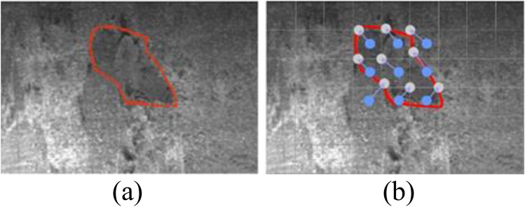
Inspired by the deformable convolutional network (DCN) [57], our proposed FDD as shown in Fig. 5 adopts the deformable convolution in the FPN module and deformable RoI pooling in the cascaded R-CNN modules to augment the spatial sampling locations in the convolution and RoI pooling modules with additional offsets, and to learn the offsets without additional supervision. The original regular convolution operation is written in Eq. (4), where denotes the input feature map, denotes the output feature map, denotes the weights, is a certain location in, and denotes a regular sampling grid. For instance, defines a kernel with a dilation rate of 1, and enumerates the locations in. In contrast, in deformable convolution, formulated as Eq. (5), the regular sampling grid is augmented by offsets which are generated by a sibling branch of the regular convolution. As shown in Fig. 6b, through deformable convolution, certain 2D offsets are added to the regular grid sampling locations in the standard convolution, which makes the convolution highly adaptive to the geometrical variation of the defect.
Fig. 6.
a The defect location. b The deformable convolution sampling the defect location
The process of deformable RoI pooling is similar to that of the deformable convolution, in which offsets are added to the spatial binning positions in the pooling operation. As shown in Eq. (6), the regular RoI pooling splits the RoI into bins and produces an feature map , where is the input, is the top-left corner location of , is the set of locations in the bin, and is the number of pixels in the bin. Then, the generated offsets are added to the spatial binning positions as in Eq. (7) to enable the deformable RoI pooling operation.
| 4 |
| 5 |
| 6 |
| 7 |
Guided anchoring RPN
In defect detection problems, we need to consider the non-uniform distribution of defect locations and shapes. Therefore, we adopt region proposal via guided anchoring (GA) [37]. It works as follows: first, the anchor location prediction branch yields a probability map to predict the locations where the center of objects of interest are likely to exist [56]. This step dramatically reduces the number of anchors compared to the sliding-window scheme. The next step is to determine the shape of the object that may exist at each location by the anchor shape prediction branch. Furthermore, an anchor-guided feature adaptation component transforms the feature at each individual location based on the underlying anchor shape, using a 3 × 3 deformable convolution layer. This makes the features and the anchors match more closely.
Loss functions
Moreover, the proposed architecture is optimized in an end-to-end training procedure that employs the sum of the GA-RPN head loss and the Cascade R-CNN loss . More specifically, the GA-RPN loss as shown in Eq. (8) is a multi-task loss, in which the conventional classification loss and regression loss are combined with the anchor localization loss (the loss to measure the center of the foreground) and the anchor shape loss (the loss to predict the best width and height of the anchor). The three-stage Cascade R-CNN loss as shown in Eq. (9) includes the classification loss and the regression loss of H1, the classification loss and the regression loss of H2, and the classification loss and the regression loss of H3. The total loss as shown in Eq. (10) is the summation of and .
| 8 |
| 9 |
| 10 |
Ultimate scaling
In the object detection task [44, 64, 67–76], multi-scale testing is employed in the inference stage to resize a test image into several scales. Each re-scaled image will go through the detection network to obtain a detection result; then, the final result is obtained using some voting mechanism. Although this method significantly increases the accuracy, it also increases the inference time. Instead of using such a multi-scale testing scheme, we propose a more efficient technique in the inference stage as shown in Fig. 4b called the “ultimate scaling.” After the model is trained, we apply the model to the training set and determine the optimal size of the training images, by trying out all sizes within the scale range of training images, with a step size of 100 pixels along the height direction. The size that leads to the highest mAP for the training set will be selected as the optimal size, and all test images are resized to this optimal size before testing. The combination of random scaling in the training stage and such ultimate scaling in the inference stage effectively improved the detection accuracy.
Experimental results
Parameter configuration and datasets
Our proposed FDD is implemented in PyTorch and trained on a single NVIDIA GeForce RTX 2080Ti GPU. The batch size is 1. The initial learning rate is set at 0.001 and is reduced by a factor of 10 when the number of epochs reaches 16 and 19. The total number of epochs is 40.
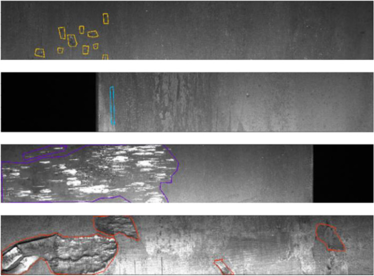
In this experiment, we use three well-known surface defect datasets. The first dataset, Severstal, is a steel defect dataset [38]. As shown in Fig. 7, it has 4 defect categories. According to a study in [77], class 1 is marked by yellow features pitted surface defects, class 2 marked by blue features crazing defects, class 3 marked by purple features scratch defects, and class 4 marked by red features patch defects. We use 5332 images and 667 images for training and testing, respectively. The original labels in this dataset are pixel-wise annotations. To perform defect detection, we converted the pixel-wise annotations into bounding box labels, in accordance with the Pascal VOC format [78].
Fig. 7.
The Severstal defect dataset
The second dataset is the Northeastern University (NEU) surface defect dataset [7], as shown in Fig. 8. It contains 1800 images, belonging to six classes of hot-rolled steel plates: crazing, inclusion, patches, pitted surface, rolled-in scales, and scratches. Following [7], we use 1260 images as the training set and 540 images as the test set. To evaluate the performance of our proposed FDD in detecting general defects in addition to steel surface defects, we also use the synthesized Deutsche Arbeitsgemeinschaft für Mustererkennung e.V., the German chapter of the International Association for Pattern Recognition (DAGM) dataset [12] as shown in Fig. 9. A total of 150 defect images are included in each of the six classes for developing surface defect inspection systems. The miscellaneous anomalies in the dataset occur on a variety of statistically textured backgrounds, as described in [77]. Anomalies vary in shape and size, making it difficult to distinguish them from complex textures. This dataset reflects real-world defects, which can demonstrate the effectiveness of our proposed method on general defects. There are 900 images in total, and we adopt 720 images for training and 180 images for testing.
Fig. 8.
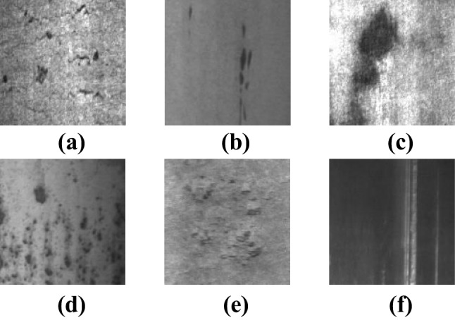
The NEU defect dataset. a Crazing. b Inclusion. c Patches. d Pitted surface. e Rolled-in scale. f Scratches
Fig. 9.
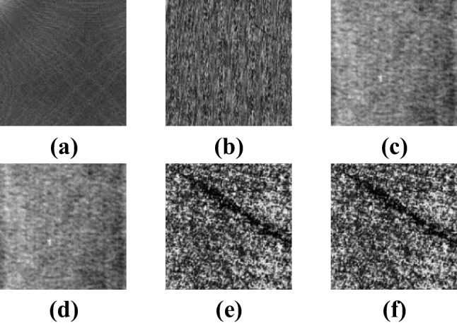
The DAGM defect dataset. a Class 1. b Class 2. c Class 3. d Class 4. e Class 5. f Class 6
Performance evaluation metrics
For each dataset, the defect detection accuracy is evaluated by the average precision (AP) of each defect class, the mean average precision (mAP) over all classes, and the average recall (AR).
For a specific defect class, the precision and recall are first calculated according to Eqs. (11) and (12), where TP, FP, and FN represent the number of true positives, false positives, and false negatives of this class, respectively. The average precision (AP) is then computed over different levels of recall achieved by varying the confidence score threshold.
| 11 |
| 12 |
Finally, we calculate the mean of the AP across all defect classes, resulting in the mAP value, and calculate the mean of the Recall across all defect classes as the AR value.
Objective performance and discussion
Table 1 shows the scaling parameters for each dataset in our experimental studies, which are applied to the random scaling in the training stage and ultimate scaling in the inference stage. We set based on the image size of three different datasets. The original images of the Severstal dataset have a high resolution: . To enrich the training set resolution, we set the initial width and height as , which are smaller than the original resolution, and set the maximum width and height () to be the same as the original size. Therefore, the size of the training images varies from small to large. The second dataset is the NEU surface defect dataset, which has small width and height (200, 200). Since small resolution images do not have a positive impact on the detection result, for this dataset, the initial width and height are set as (500, 500) and the maximum width and height () are set as (1200, 1200). The third dataset is DAGM for general defects, which has a medium resolution: the original width and height ( are (512, 512). For this dataset, the initial width and height () are set as (400, 400), and the maximum width and height () are set as (1200, 1200). This range allows the network to learn from lower to higher resolution images.
Table 1.
The scaling set parameters
| Datasets | ||||||
|---|---|---|---|---|---|---|
| Severstal | 1600 | 256 | 625 | 100 | 1600 | 256 |
| NEU | 200 | 200 | 500 | 500 | 1200 | 1200 |
| DAGM | 512 | 512 | 400 | 400 | 1200 | 1200 |
A validation study of each component of the proposed FDD model was conducted on the Severstal dataset, as shown in Table 2. We adopt Cascade R-CNN [32] with a ResNet-50 backbone [79] as the baseline, which achieves an AR of 85.5% and an mAP of 67.5%. By adding the proposed preprocessing blocks (including random scaling) and ultimate scaling, the AR and mAP are improved to 96.7% and 72.2%, respectively. This illustrates the benefit of the proposed random scaling operation in the training stage, which enhances the variation defect features. Additionally, the ultimate scaling can be used in the testing stage to select the optimal size for the input image. After integrating the proposed deformable convolution, deformable RoI pooling, and guided anchoring region proposal network (GA-RPN), the AR and mAP further increased to 96.9% and 78.3%. This improved accuracy was attributable to the deformable operation that adapted to the geometric variation of the defect shape and precisely localized the bounding box with GA-RPN.
Table 2.
The ablation study for accuracy improvement of FDD
| Models | Improvement | REC-1 | REC-2 | REC-3 | REC-4 | AP-1 | AP-2 | AP-3 | AP-4 | AR | mAP |
|---|---|---|---|---|---|---|---|---|---|---|---|
| Cascade R-CNN | Baseline Resnet50 | 0.802 | 0.850 | 0.878 | 0.891 | 0.608 | 0.714 | 0.684 | 0.696 | 0.855 | 0.675 |
| + Proposed preprocessing blocks and ultimate scaling | 0.942 | 0.950 | 0.976 | 1.000 | 0.600 | 0.788 | 0.712 | 0.785 | 0.967 | 0.722 | |
| + Deformable operation and guided anchoring RPN | 0.953 | 0.950 | 0.973 | 1.000 | 0.703 | 0.746 | 0.833 | 0.852 | 0.969 | 0.783 |
In Tables 3, 4 and 5, we objectively compare the performance of our proposed FDD method to state-of-the-art methods: YOLOv4 [26], YOLOv5 [27], YOLOX [28], PVTv2 [25], DetectoRS [33], DDN [7], CP-YOLOv3-dense [31], DEA_RetinaNet [30], DIN [34], DCC-CenterNet [29], and Deep Reg [12]. Our proposed method outperformed these methods by significant margins in terms of the AR and mAP values.
Table 3.
Comparison results for the Severstal dataset
| Models | Backbone network | REC-1 | REC-2 | REC-3 | REC-4 | AP-1 | AP-2 | AP-3 | AP-4 | AR | mAP |
|---|---|---|---|---|---|---|---|---|---|---|---|
| YOLOv4 [26] | CSPDarknet | 0.895 | 0.850 | 0.949 | 0.922 | 0.443 | 0.615 | 0.664 | 0.710 | 0.904 | 0.608 |
| YOLOv5 [27] | CSPDarknet | 0.837 | 0.900 | 0.921 | 0.906 | 0.423 | 0.693 | 0.607 | 0.682 | 0.891 | 0.601 |
| YOLOX [28] | CSPDarknet | 0.802 | 0.900 | 0.921 | 0.828 | 0.529 | 0.628 | 0.745 | 0.707 | 0.863 | 0.652 |
| PVTv2 [25] | PVTv2-B5 | 0.895 | 0.850 | 0.934 | 0.953 | 0.579 | 0.637 | 0.779 | 0.856 | 0.908 | 0.713 |
| DetectoRS [33] | Resnet-50 | 0.791 | 0.850 | 0.870 | 0.938 | 0.644 | 0.812 | 0.788 | 0.864 | 0.862 | 0.777 |
| Cascade R-CNN [32] | Resnet-50 | 0.802 | 0.850 | 0.878 | 0.891 | 0.608 | 0.714 | 0.684 | 0.696 | 0.855 | 0.675 |
| FDD (Proposed) | Resnet-50 | 0.953 | 0.950 | 0.973 | 1.000 | 0.703 | 0.746 | 0.833 | 0.852 | 0.969 | 0.783 |
Table 4.
Comparison results for the NEU dataset
| Models | Backbone network | AP crazing | AP inclusion | AP patches | AP pitted_surface | AP rolled-in_scale | AP scratches | AR | mAP |
|---|---|---|---|---|---|---|---|---|---|
| DDN [7] | Resnet-50 | 0.620 | 0.847 | 0.907 | 0.897 | 0.763 | 0.901 | - | 0.823 |
| CP-YOLOv3-dense [31] | Darknet + DenseNet | 0.353 | 0.824 | 0.919 | 0.828 | 0.777 | 0.902 | 0.823 | 0.767 |
| DEA_RetinaNet [30] | Resnet-152 | 0.609 | 0.825 | 0.943 | 0.958 | 0.672 | 0.741 | - | 0.791 |
| DIN [34] | Resnet-50 | 0.614 | 0.856 | 0.930 | 0.903 | 0.646 | 0.833 | - | 0.805 |
| DCC-CenterNet [29] | Resnet-50 | 0.457 | 0.851 | 0.900 | 0.825 | 0.707 | 0.958 | - | 0.794 |
| Cascade R-CNN [32] | Resnet-50 | 0.492 | 0.871 | 0.906 | 0.885 | 0.686 | 0.904 | 0.957 | 0.793 |
| FDD (Proposed) | Resnet-50 | 0.622 | 0.890 | 0.924 | 0.880 | 0.749 | 0.937 | 0.997 | 0.834 |
Table 5.
Comparison results for the DAGM dataset
Table 3 shows the proposed methods achieved an AR of 96.9% and an mAP of 78.3% on top of the ResNet-50 backbone, thus surpassing the accuracy of YOLOv4 [26], YOLOv5 [27], YOLOX [28], PVTv2 [25], and DetectoRS [33].
Table 4 shows the comparison study on the NEU steel surface defect dataset. The optimal test image size is chosen as during the ultimate scaling process. The DDN [7], DIN [34], and DCC-CenterNet [29] models run on the standard backbone (ResNet-50) and achieved an mAP of 82.3%, 80.5%, and 79.4%, respectively. The Cascade R-CNN [32] also adopted the ResNet-50 backbone and achieved an AR of 95.7% and an mAP of 79.3%. DEA_RetinaNet run on top of a deeper backbone ResNet-152 and achieved an mAP of 79.1%. On the other hand, the CP-YOLOv3-dense model [31] integrated YOLOv3 with the DenseNet backbone to achieve an AR of 82.3% and an mAP of 76.7%. In contrast, although our proposed FDD is implemented with the standard ResNet-50 backbone, it achieved the highest mAP of 83.4% and the highest AR of 99.7% among all methods in comparison.
With the aim to develop a widely applicable defect detection system, the proposed method was also tested on the DAGM dataset with an image size of as chosen by the ultimate scaling scheme. This experiment mimics a real-world defect detection scenario. As shown in Table 5, the segmentation-based defect detection system Deep Reg [12] achieved an AR of 99% and an mAP of 98% on this dataset. On the other hand, the Cascade R-CNN [32] achieved an AR of 99.7% and an mAP of 98.7%. The proposed FDD achieved an AR of 100% and an mAP of 100%, when it is implemented with the ResNet-50 backbone.
Moreover, in Table 6, the proposed FDD with the ResNet-50 backbone achieved an inference speed of 12 frames per second (fps) on a single NVIDIA GeForce RTX 2080Ti GPU, which is on par with that of the state-of-the-art feature pyramid networks model DetectoRS [33] and also meets the criteria of steel surface inspection systems as explained in [39, 40], where the inference speed must be greater than or equal to 10 fps. Although the other existing methods in Table 6 achieve higher speeds, we demonstrated in Tables 3, 4 and 5 that they have lower detection accuracy than our proposed FDD.
Table 6.
Comparison results for run time
Subjective performance and discussion
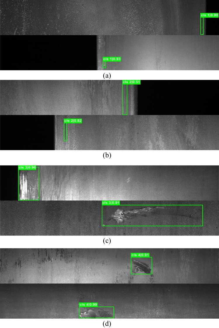
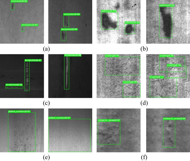
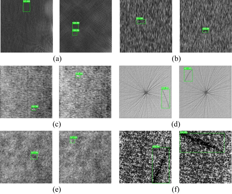
Figures 10, 11 and 12 show sample testing results to demonstrate the subjective performance of the proposed FDD. The system shows accurately detected defects from small and medium to larger scales. Each image shown in Figs. 10, 11 and 12 contains a green bounding box, which indicates the location of the detected defect along with its predicted class label.
Fig. 10.
Detection results for the Severstal defect dataset: a class 1, b class 2, c class 3, and d class 4
Fig. 11.
The sample detection results on the NEU defect dataset: a inclusion, b patches, c scratches, d crazing, e pitted surface, and f rolled-in scale
Fig. 12.
The sample detection results on the DAGM dataset: a class 1, b class 2, c class 3, d class 4, e class 5, and f class 6
Figure 10 shows that our proposed model accurately predicts the four classes of defects in the Severstal dataset. The defects in this dataset are quite challenging since they appear in varying scales. Classes 1 and 2 shown in Fig. 10 a and b belong to small defects, while classes 3 and 4 shown in Fig. 10 c and d belong to larger defects. Figure 10 demonstrates that the proposed system can not only detect defects of various scales, but also accurately predict the defect locations when the defective pixels are similar to the background.
Figure 11 shows the detection results on the NEU defect dataset. This dataset is a very common dataset in the steel surface inspection system. Among the six classes of defects, the inclusion, patches, and scratches are defects of varying scales. On the other hand, the crazing, pitted surface, and rolled-in scale defects have pixels that are similar to background pixels.
To demonstrate that our proposed FDD model can detect general defects, in Fig. 12, we tested our model on the DAGM dataset. The results show that our model accurately localized six classes of defects with different textures.
Conclusion
In this paper, we design a new defect detection system called the FDD. We propose the novel concepts of random scaling in the data preprocessing pipeline for training and ultimate scaling for testing and combine them with an improved cascade R-CNN detector, which involves deformable convolution, deformable RoI pooling, and a guided anchoring RPN. The resulting FDD system is used in the defect detection field for the first time in the literature. The experimental results demonstrate that the proposed model has significantly improved the defect detection accuracy on steel surface defect datasets and a general defect dataset compared to existing methods, while maintaining the processing speed criteria required for steel surface inspection systems. In further work, we will extend our network structure to a more generalized defect detector.
Author contribution
The systems and experiments were designed by Fityanul Akhyar; the data analysis was done by Chao-Yung Hsu; the paper was revised by Ying Liu, and Timothy K. Shih; and the research was conducted by Chih-Yang Lin.
Funding
This work was supported by the National Science and Technology Council, Taiwan, under Grant MOST 110–2221-E-155–039-MY3, and Grant MOST 111–2221-E155-039-MY3. The National Science Foundation also partially supported this work under grant number ECCS-2138635.
Data availability
The datasets analyzed during the current article are available on the Kaggle platform (https://www.kaggle.com/c/severstal-steel-defect-detection (accessed on October 14th, 2022)) provided by Severstal steel and mining industry, (http://faculty.neu.edu.cn/yunhyan/NEU surface defect database.html (accessed on October 14th, 2022)) provided by North Eastern University (NEU) Steel Surface Defects Database and (https://conferences.mpi-inf.mpg.de/dagm/2007/prizes.html (accessed on October 14th, 2022)) 2007 symposium of the DAGM (Deutsche Arbeitsgemeinschaft f¨ur Mustererkennung e.V., the German chapter of the International Association for Pattern Recognition).
Code availability
Not applicable.
Declarations
Ethical approval
This article does not contain any studies with human participants performed by any of the authors. Consent to participate Informed consent was obtained from all individual participants included in the study.
Consent for publication
The participant has consented to the submission of the case report to the journal.
Competing interests
The authors declare no competing interests.
Footnotes
Publisher's note
Springer Nature remains neutral with regard to jurisdictional claims in published maps and institutional affiliations.
Contributor Information
Fityanul Akhyar, Email: fityanul@telkomuniversity.ac.id.
Ying Liu, Email: yliu15@scu.edu.
Chao-Yung Hsu, Email: cyhsu2006@gmail.com.
Timothy K. Shih, Email: timothykshih@gmail.com
Chih-Yang Lin, Email: andrewlin@ncu.edu.tw.
References
- 1.Li Z, Yang Q (2011) System design for PCB defects detection based on AOI technology. 2011 4th International Congress on Image and Signal Processing: IEEE, p. 1988–91
- 2.Guo M, Wang R (2016) The introduction of AOI in PCB defect detection based on linear array camera. 2016 International Forum on Management, Education and Information Technology Application: Atlantis Press
- 3.Fan KC, Hsu C. Strategic planning of developing automatic optical inspection (AOI) technologies in Taiwan. J Phys Confer Ser. 2005;13(1):394. doi: 10.1088/1742-6596/13/1/090. [DOI] [Google Scholar]
- 4.Peres RS, Jia X, Lee J, Sun K, Colombo AW, Barata J. Industrial artificial intelligence in industry 4.0-systematic review, challenges and outlook. IEEE Access. 2020;8:220121–39. doi: 10.1109/ACCESS.2020.3042874. [DOI] [Google Scholar]
- 5.Akhyar F, Lin C-Y, Muchtar K, Wu T-Y, Ng H-F (2019) High efficient single-stage steel surface defect detection. 2019 16th IEEE International Conference on Advanced Video and Signal Based Surveillance (AVSS): IEEE, p. 1–4
- 6.Dong H, Song K, He Y, Xu J, Yan Y, Meng Q. PGA-Net: Pyramid feature fusion and global context attention network for automated surface defect detection. IEEE Trans Indust Inform. 2019;16(12):7448–7458. doi: 10.1109/TII.2019.2958826. [DOI] [Google Scholar]
- 7.He Y, Song K, Meng Q, Yan Y. An end-to-end steel surface defect detection approach via fusing multiple hierarchical features. IEEE Trans Instrum Meas. 2019;69(4):1493–1504. doi: 10.1109/TIM.2019.2915404. [DOI] [Google Scholar]
- 8.Lin C-Y, Chen C-H, Yang C-Y, Akhyar F, Hsu C-Y, Ng H-F (2019) Cascading convolutional neural network for steel surface defect detection. International Conference on Applied Human Factors and Ergonomics: Springer p. 202–12
- 9.Zhang C, Shi W, Li X, Zhang H. Improved bare PCB defect detection approach based on deep feature learning. J Eng. 2018;16:1415–1420. doi: 10.1049/joe.2018.8275. [DOI] [Google Scholar]
- 10.Ding R, Dai L, Li G, Liu H. TDD-net: a tiny defect detection network for printed circuit boards. CAAI Trans Intell Technol. 2019;4(2):110–116. doi: 10.1049/trit.2019.0019. [DOI] [Google Scholar]
- 11.Hu B, Wang J. Detection of PCB surface defects with improved faster-RCNN and feature pyramid network. IEEE Access. 2020;8:108335–108345. doi: 10.1109/ACCESS.2020.3001349. [DOI] [Google Scholar]
- 12.He Z, Liu Q. Deep regression neural network for industrial surface defect detection. IEEE Access. 2020;8:35583–35591. doi: 10.1109/ACCESS.2020.2975030. [DOI] [Google Scholar]
- 13.Ren R, Hung T, Tan KC. A generic deep-learning-based approach for automated surface inspection. IEEE Trans Cybern. 2017;48(3):929–940. doi: 10.1109/TCYB.2017.2668395. [DOI] [PubMed] [Google Scholar]
- 14.Li L, Ota K, Dong M. Deep learning for smart industry: efficient manufacture inspection system with fog computing. IEEE Trans Industr Inf. 2018;14(10):4665–4673. doi: 10.1109/TII.2018.2842821. [DOI] [Google Scholar]
- 15.Wang J, Fu P, Gao RX. Machine vision intelligence for product defect inspection based on deep learning and Hough transform. J Manuf Syst. 2019;51:52–60. doi: 10.1016/j.jmsy.2019.03.002. [DOI] [Google Scholar]
- 16.Lin H, Li B, Wang X, Shu Y, Niu S. Automated defect inspection of LED chip using deep convolutional neural network. J Intell Manuf. 2019;30(6):2525–2534. doi: 10.1007/s10845-018-1415-x. [DOI] [Google Scholar]
- 17.Mentouri Z, Doghmane H, Moussaoui A, Boudjehem D (2020) Surface flaw classification based on dual cross pattern. 2020 1st International Conference on Communications, Control Systems and Signal Processing (CCSSP): IEEE p. 137–41.
- 18.Mentouri Z, Doghmane H, Moussaoui A, Bourouba H. Improved cross pattern approach for steel surface defect recognition. Int J Adv Manuf Technol. 2020;110(11–12):3091–3100. doi: 10.1007/s00170-020-06050-x. [DOI] [Google Scholar]
- 19.Mentouri Z, Moussaoui A, Boudjehem D, Doghmane H. Steel strip surface defect identification based on binarized statistical features. Sci Bullet Ser B: Chem Mater Sci. 2018;80(4):1–12. [Google Scholar]
- 20.Song K, Hu S, Yan Y. Automatic recognition of surface defects on hot-rolled steel strip using scattering convolution network. J Comput Inf Syst. 2014;10(7):3049–3055. [Google Scholar]
- 21.Yi L, Li G, Jiang M. An end-to-end steel strip surface defects recognition system based on convolutional neural networks. Steel Res Int. 2017;88(2):1600068. doi: 10.1002/srin.201600068. [DOI] [Google Scholar]
- 22.Su B, Chen H, Chen P, Bian G, Liu K, Liu W. Deep learning-based solar-cell manufacturing defect detection with complementary attention network. IEEE Trans Indust Inform. 2020;17(6):4084–4095. doi: 10.1109/TII.2020.3008021. [DOI] [Google Scholar]
- 23.Li Y, Xu J (2020) Electronic product surface defect detection based on a MSSD Network. 2020 IEEE 4th Information Technology, Networking, Electronic and Automation Control Conference (ITNEC): IEEE p. 773–7
- 24.Zhao Z-Q, Zheng P, Xu S-t, Wu X. Object detection with deep learning: a review. IEEE Trans Neural Networks Learn Syst. 2019;30(11):3212–32. doi: 10.1109/TNNLS.2018.2876865. [DOI] [PubMed] [Google Scholar]
- 25.Wang W, Xie E, Li X, Fan D-P, Song K, Liang D, et al (2021) Pvtv2: improved baselines with pyramid vision transformer. arXiv preprint arXiv:210613797
- 26.Bochkovskiy A, Wang C-Y, Liao H-YM (2020) Yolov4: optimal speed and accuracy of object detection. arXiv preprint arXiv:200410934
- 27.GitHub (2021) YOLOV5-Master. https://github.com/ultralytics/yolov5.git/. Accessed 14 Oct 2022
- 28.Ge Z, Liu S, Wang F, Li Z, Sun J (2021) Yolox: exceeding yolo series in 2021. arXiv preprint arXiv:210708430
- 29.Tian R, Jia M. DCC-CenterNet: a rapid detection method for steel surface defects. Measurement. 2022;187:110211. doi: 10.1016/j.measurement.2021.110211. [DOI] [Google Scholar]
- 30.Cheng X, Yu J. RetinaNet with difference channel attention and adaptively spatial feature fusion for steel surface defect detection. IEEE Trans Instrum Meas. 2020;70:1–11. [Google Scholar]
- 31.Zhang J, Kang X, Ni H, Ren F. Surface defect detection of steel strips based on classification priority YOLOv3-dense network. Ironmak Steelmak. 2021;48(5):547–558. doi: 10.1080/03019233.2020.1816806. [DOI] [Google Scholar]
- 32.Cai Z, Vasconcelos N (2018) Cascade r-cnn: Delving into high quality object detection. Proceedings of the IEEE conference on computer vision and pattern recognition p. 6154–62.
- 33.Qiao S, Chen L-C, Yuille A (2020) DetectoRS: detecting objects with recursive feature pyramid and switchable atrous convolution. arXiv preprint arXiv:200602334
- 34.Hao R, Lu B, Cheng Y, Li X, Huang B. A steel surface defect inspection approach towards smart industrial monitoring. J Intell Manuf. 2021;32(7):1833–1843. doi: 10.1007/s10845-020-01670-2. [DOI] [Google Scholar]
- 35.Qian K (2019) Automated detection of steel defects via machine learning based on real-time semantic segmentation. Proceedings of the 3rd International Conference on Video and Image Processing. p. 42–6
- 36.Chen K, Pang J, Wang J, Xiong Y, Li X, Sun S, et al (2019) Hybrid task cascade for instance segmentation. Proceedings of the IEEE conference on computer vision and pattern recognition. p. 4974–83.
- 37.Wang J, Chen K, Yang S, Loy CC, Lin D (2019) Region proposal by guided anchoring. Proceedings of the IEEE Conference on Computer Vision and Pattern Recognition. p. 2965–74.
- 38.Kaggle (2019) Severstal: steel defect detection. https://www.kaggle.com/c/severstal-steel-defect-detection/overview. Accessed 14 Oct 2022
- 39.Sun X, Gu J, Tang S, Li J. Research progress of visual inspection technology of steel products—a review. Appl Sci. 2018;8(11):2195. doi: 10.3390/app8112195. [DOI] [Google Scholar]
- 40.Wan X, Zhang X, Liu L. An improved VGG19 transfer learning strip steel surface defect recognition deep neural network based on few samples and imbalanced datasets. Appl Sci. 2021;11(6):2606. doi: 10.3390/app11062606. [DOI] [Google Scholar]
- 41.Redmon J, Farhadi A (2018) Yolov3: an incremental improvement. arXiv preprint arXiv:180402767
- 42.Wang C-Y, Liao H-YM, Wu Y-H, Chen P-Y, Hsieh J-W, Yeh I-H (2020) CSPNet: a new backbone that can enhance learning capability of CNN. Proceedings of the IEEE/CVF conference on computer vision and pattern recognition workshops. p. 390–1.
- 43.He K, Zhang X, Ren S, Sun J. Spatial pyramid pooling in deep convolutional networks for visual recognition. IEEE Trans Pattern Anal Mach Intell. 2015;37(9):1904–1916. doi: 10.1109/TPAMI.2015.2389824. [DOI] [PubMed] [Google Scholar]
- 44.Liu S, Qi L, Qin H, Shi J, Jia J (2018) Path aggregation network for instance segmentation. Proceedings of the IEEE conference on computer vision and pattern recognition. p. 8759–68.
- 45.Huang G, Liu S, Van der Maaten L, Weinberger KQ (2018) Condensenet: an efficient densenet using learned group convolutions. Proceedings of the IEEE conference on computer vision and pattern recognition. p. 2752–61.
- 46.Qin Y, Xing Y, Du J (2020) LSDDN: a lightweight end-to-end network for surface defect detection. Proceedings of the 2020 the 4th International Conference on Innovation in Artificial Intelligence. p. 79–83.
- 47.Lin T-Y, Goyal P, Girshick R, He K, Dollár P (2017) Focal loss for dense object detection. Proceedings of the IEEE international conference on computer vision. p. 2980–8.
- 48.Duan K, Bai S, Xie L, Qi H, Huang Q, Tian Q. Centernet: keypoint triplets for object detection. Proceedings of the IEEE/CVF International Conference on Computer Vision2019. p. 6569–78.
- 49.Vaswani A, Shazeer N, Parmar N, Uszkoreit J, Jones L, Gomez AN, Kaiser L, Polosukhin I (2017) Attention is all you need. Adv Neur Inform Process Syst 30. 10.48550/arXiv.1706.03762
- 50.Dosovitskiy A, Beyer L, Kolesnikov A, Weissenborn D, Zhai X, Unterthiner T, et al (2020) An image is worth 16x16 words: transformers for image recognition at scale. arXiv preprint arXiv:201011929
- 51.Strudel R, Garcia R, Laptev I, Schmid C (2021) Segmenter: transformer for semantic segmentation. Proceedings of the IEEE/CVF international conference on computer vision. p. 7262–72.
- 52.Xie E, Wang W, Yu Z, Anandkumar A, Alvarez JM, Luo P. SegFormer: Simple and efficient design for semantic segmentation with transformers. Adv Neural Inf Process Syst. 2021;34:12077–12090. [Google Scholar]
- 53.Wang W, Xie E, Li X, Fan D-P, Song K, Liang D, et al (2021) Pyramid vision transformer: a versatile backbone for dense prediction without convolutions. Proceedings of the IEEE/CVF international conference on computer vision. p. 568–78
- 54.Wang W, Xie E, Li X, Fan D-P, Song K, Liang D, et al (2021) Pyramid vision transformer: a versatile backbone for dense prediction without convolutions. arXiv preprint arXiv:210212122.
- 55.Lin T-Y, Dollár P, Girshick R, He K, Hariharan B, Belongie S (2017) Feature pyramid networks for object detection. Proceedings of the IEEE conference on computer vision and pattern recognition. p. 2117–25
- 56.Ren S, He K, Girshick R, Sun J (2015) Faster r-cnn: towards real-time object detection with region proposal networks. Adv Neur Inform Process Syst 28. 10.48550/arXiv.1506.01497 [DOI] [PubMed]
- 57.Dai J, Qi H, Xiong Y, Li Y, Zhang G, Hu H, et al (2017) Deformable convolutional networks. Proceedings of the IEEE international conference on computer vision. p. 764–73
- 58.Pang J, Chen K, Shi J, Feng H, Ouyang W, Lin D (2019) Libra r-cnn: towards balanced learning for object detection. Proceedings of the IEEE/CVF Conference on Computer Vision and Pattern Recognition. p. 821–30
- 59.Girshick R (2015) Fast r-cnn. Proceedings of the IEEE international conference on computer vision. p. 1440–8
- 60.Akhyar F, Lin C-Y, Kathiresan GS (2021) A beneficial dual transformation approach for deep learning networks used in steel surface defect detection. Proceedings of the 2021 International Conference on Multimedia Retrieval. p. 619–22
- 61.Xie S, Girshick R, Dollár P, Tu Z, He K (2017) Aggregated residual transformations for deep neural networks. Proceedings of the IEEE conference on computer vision and pattern recognition. p. 1492–500
- 62.Simonyan K, Zisserman A (2014) Very deep convolutional networks for large-scale image recognition. arXiv preprint arXiv:14091556
- 63.Everingham M, Van Gool L, Williams CK, Winn J, Zisserman A. The pascal visual object classes (VOC) challenge. Int J Comput Vision. 2010;88(2):303–338. doi: 10.1007/s11263-009-0275-4. [DOI] [Google Scholar]
- 64.Singh B, Najibi M, Davis LS (2018) Sniper: efficient multi-scale training. Advances in neural information processing systems. p. 9310–20
- 65.Chen K, Wang J, Pang J, Cao Y, Xiong Y, Li X, et al (2019) MMDetection: open mmlab detection toolbox and benchmark. arXiv preprint arXiv:190607155
- 66.Farooq M, Hafeez A (2020) Covid-resnet: a deep learning framework for screening of covid19 from radiographs. arXiv preprint arXiv:200314395
- 67.Singh B, Davis LS (2018) An analysis of scale invariance in object detection snip. Proceedings of the IEEE conference on computer vision and pattern recognition. p. 3578–87
- 68.Zhou X, Zhuo J, Krahenbuhl P (2019) Bottom-up object detection by grouping extreme and center points. Proceedings of the IEEE Conference on Computer Vision and Pattern Recognition. p. 850–9
- 69.Law H, Deng J (2018) Cornernet: detecting objects as paired keypoints. Proceedings of the European Conference on Computer Vision (ECCV). p. 734–50
- 70.Zhu X, Hu H, Lin S, Dai J (2019) Deformable convnets v2: more deformable, better results. Proceedings of the IEEE Conference on Computer Vision and Pattern Recognition. p. 9308–16
- 71.Tian Z, Shen C, Chen H, He T (2019) Fcos: fully convolutional one-stage object detection. Proceedings of the IEEE international conference on computer vision. p. 9627–36
- 72.Zhu C, He Y, Savvides M (2019) Feature selective anchor-free module for single-shot object detection. Proceedings of the IEEE Conference on Computer Vision and Pattern Recognition. p. 840–9
- 73.Peng C, Xiao T, Li Z, Jiang Y, Zhang X, Jia K, et al (2018) Megdet: a large mini-batch object detector. Proceedings of the IEEE Conference on Computer Vision and Pattern Recognition. p. 6181–9
- 74.Zhou X, Wang D, Krähenbühl P (2019) Objects as points. arXiv preprint arXiv:190407850
- 75.Song G, Liu Y, Wang X (2020) Revisiting the sibling head in object detector. Proceedings of the IEEE/CVF Conference on Computer Vision and Pattern Recognition. p. 11563–72
- 76.Li Y, Chen Y, Wang N, Zhang Z (2019) Scale-aware trident networks for object detection. Proceedings of the IEEE international conference on computer vision. p. 6054–63
- 77.Wan Q, Gao L, Li X, Wen L. Industrial image anomaly localization based on Gaussian clustering of pretrained feature. IEEE Trans Industr Electron. 2021;69(6):6182–6192. doi: 10.1109/TIE.2021.3094452. [DOI] [Google Scholar]
- 78.Everingham M, Eslami SA, Van Gool L, Williams CK, Winn J, Zisserman A. The pascal visual object classes challenge: a retrospective. Int J Comput Vision. 2015;111(1):98–136. doi: 10.1007/s11263-014-0733-5. [DOI] [Google Scholar]
- 79.He K, Zhang X, Ren S, Sun J (2016) Deep residual learning for image recognition. Proceedings of the IEEE conference on computer vision and pattern recognition. p. 770–8
Associated Data
This section collects any data citations, data availability statements, or supplementary materials included in this article.
Data Availability Statement
The datasets analyzed during the current article are available on the Kaggle platform (https://www.kaggle.com/c/severstal-steel-defect-detection (accessed on October 14th, 2022)) provided by Severstal steel and mining industry, (http://faculty.neu.edu.cn/yunhyan/NEU surface defect database.html (accessed on October 14th, 2022)) provided by North Eastern University (NEU) Steel Surface Defects Database and (https://conferences.mpi-inf.mpg.de/dagm/2007/prizes.html (accessed on October 14th, 2022)) 2007 symposium of the DAGM (Deutsche Arbeitsgemeinschaft f¨ur Mustererkennung e.V., the German chapter of the International Association for Pattern Recognition).
Not applicable.


