

Abstract
Motivation
To develop and assess the accuracy of deep learning models that identify different retinal cell types, as well as different retinal ganglion cell (RGC) subtypes, based on patterns of single-cell RNA sequencing (scRNA-seq) in multiple datasets.
Results
Deep domain adaptation models were developed and tested using three different datasets. The first dataset included 44 808 single retinal cells from mice (39 cell types) with 24 658 genes, the second dataset included 6225 single RGCs from mice (41 subtypes) with 13 616 genes and the third dataset included 35 699 single RGCs from mice (45 subtypes) with 18 222 genes. We used four loss functions in the learning process to align the source and target distributions, reduce misclassification errors and maximize robustness. Models were evaluated based on classification accuracy and confusion matrix. The accuracy of the model for correctly classifying 39 different retinal cell types in the first dataset was ∼92%. Accuracy in the second and third datasets reached ∼97% and 97% in correctly classifying 40 and 45 different RGCs subtypes, respectively. Across a range of seven different batches in the first dataset, the accuracy of the lead model ranged from 74% to nearly 100%. The lead model provided high accuracy in identifying retinal cell types and RGC subtypes based on scRNA-seq data. The performance was reasonable based on data from different batches as well. The validated model could be readily applied to scRNA-seq data to identify different retinal cell types and subtypes.
Availability and implementation
The code and datasets are available on https://github.com/DM2LL/Detecting-Retinal-Cell-Classes-and-Ganglion-Cell-Subtypes. We have also added the class labels of all samples to the datasets.
Supplementary information
Supplementary data are available at Bioinformatics online.
1 Introduction
Single-cell technologies have substantially improved our understanding on the presence of different cell types in tissue, their divergent functions (Williams and Moody, 2003), and their sensitivity to diseases (Chalupa and Williams, 2008; Zareparsi et al., 2004). Significant efforts are currently being focused on generating human and murine cell atlases (Geisert and Williams, 2008). However, all these attempts are highly dependent on the accuracy, repeatability and reproducibility of computational and experimental workflows of single-cell RNA sequencing (scRNA-seq) analysis. There are many challenges in evaluating complex experimental workflows and the computational reproducibility of scRNA-seq methods and the joint analysis of large multiplex datasets (Łabaj and Kreil, 2016; Williams et al., 1993).
Many neuronal types and subtypes are yet to be identified in the attempt to disentangle the complex connectome of the central nervous system (CNS) (Macosko et al., 2015). Retina, part of CNS, is the home to retinal ganglion cells (RGCs), for which we have knowledge of more subtypes as compared to other neural cells (Macosko et al., 2015; Rheaume et al., 2018). The neural retina consists of five major classes of CNS neurons: photoreceptors, horizontal cells, bipolar cells, amacrine cells and RGCs, and each is characterized by morphological, physiological and molecular criteria (Seung and Sümbül, 2014). RGCs are the only projection neurons of the retina. Despite the key role of RGCs in information transmission, they account for only about 1–3% of retinal cells in most vertebrate species (Levin, 2005; Rokicki et al., 2007). However, RGCs are themselves highly heterogeneous in terms of their receptive field functions and firing dynamics, their CNS target fields, their size, their molecular subtypes and most important to us, the sensitivity to neurodegeneration in association with glaucoma (Tanabe and Jessell, 1996).
Studies going back to the era of Cajal have identified well over 30 different subtypes of RGCs. Even in nocturnal species that do not have heavy reliance on vision, such as mouse, there is an impressive number of RGC subtypes, each with unique functional properties. A systematic scRNA-seq study has highlighted close to 40 RGC molecular subtypes, and many of these subtypes also have well-known classical cell morphologies (Rheaume et al., 2018). Another recent study on single-cell profiles of RGCs introduced 45 different RGC subtypes (Tran et al., 2019).
Recent advances in scRNA-seq technologies and computational models have allowed the identification and characterization of retinal cell types and RGC subtypes based on transcriptome patterns (Daniszewski et al., 2018). However, it is challenging to transfer cell labels, which are typically identified using an unsupervised model between two studies. Another challenge is to understand the effect of intrinsic systemic bias, such as batch effect, on the labeling of one study and how it may impact new cell labeling. As such, methods that can address integration of datasets from different studies, and propagation of labels from one reference study to another study, while mitigating the batch effect, are currently of high interest. Such models could assist in generating large and complex atlases of human cells based on data from different studies (Ding and Regev, 2021; Lukowski et al., 2019).
Classic cell-type annotation approaches utilize three general steps: first, clustering the cell population; second, finding marker genes that are specific to each cluster by differential expression analysis; and finally, annotating cells corresponding to the ontological attributes of their genes (Johnson et al., 2019).
Many scRNAseq studies contain several different batches that are generated and then combined. Seurat v2 (Seurat-CCA) (Butler et al., 2018) and mnnCorrect (Haghverdi et al., 2018) were among the first approaches to address issues related to merging of scRNA-seq data from different batches. Seurat v2 utilizes canonical correlation analysis to map cells to a common low-dimensional subspace to reduce the batch effect. mnnCorrect applies mutual nearest neighbor (MNN) to calculate the heterogeneity between different batches and identify similar cell types through MNN pairs. A related approach, Seurat v3 (Stuart et al., 2019), utilizes MNN pairs between the source domain batch and target domain batch to identify ‘anchors’ in the source domain batch. ‘Anchors’ express cells in a common biological condition across different batches and are further utilized for the batch correction process by canonical correlation analysis.
Other approaches include, scVI (Lopez et al., 2018), which applies a deep learning approach to approximate the expression profile distributions in order to reduce the scRNA-seq batch effect. BERMUDA (Wang et al., 2019) is a domain adaptation method for scRNA-seq data, which uses the similarities among cell clusters to match corresponding cells and remove the batch effect by using deep auto-encoders. LAmbDA (Johnson et al., 2019) is a label-ambiguous domain adaptation model, which introduces a semi-supervised approach to test multiple machine learning algorithms including Feedforward 1 Layer neural network (NN) (FF1), Feedforward 3 Layer NN (FF3), logistic regression (LR), Random Forest (RF), Recurrent NN (RNN1) and the ensemble approach FF1 with bagging technique (FF1bag) for subtype identification and matching.
There are also supervised approaches for identifying cell types from scRNA-seq data as well. CHETAH (De Kanter et al., 2019) is a cell type identification method that measures the similarity among different cell types based on Spearman correlation and employs average linkage to generate the classification tree. CaSTLe (Lieberman et al., 2018) is a single cells classification method which utilizes the transfer learning approach to obtain information from scRNA-seq data to build important features for XGBoost classification model. scPred is a single-cell prediction approach which is based on an Support Vector Machine (SVM) with a radial kernel function (Alquicira-Hernandez et al., 2019). SingleR is the other single cells classification method which finds nearest cell types based on Spearman correlation (Aran et al., 2019).
Quick mapping of new cells based on reference cells in a well-annotated reference dataset is challenging and remains an active area of research (Cao et al., 2020). One approach could be projecting cells in the reference and new dataset into a joint embedding to find labels of the new data. In this article, we introduce a novel, deep transfer learning model for retinal cell type and RGC subtype detection based on scRNA-seq data. We harvest the advantages of deep transfer learning and domain adaptation to propagate labels from the source domain to the target domain while mitigating the batch effect. We then evaluate the model based on three independent datasets with large numbers of single retinal cells and RGCs and assess the performance based on multiple objective metrics and compare the model against several other models.
2 Materials and methods
2.1 Datasets
The first dataset from Macosko et al. study (Macosko et al., 2015) included 44 808 single cells from 39 different retinal cell types (and subtypes) with 24 658 common genes based on Droplet-based RNA-seq technology. Cells in this dataset were collected from retinas of 14-day-old wild-type C57BL/6 mice, which are genetically identical (within each strain) and exhibit a high degree of uniformity in their inherited characteristics and response to experimental treatments. As the most used inbred strain in research, genetic experiments from different labs based on this strain could be compared. As the authors wanted to generate a large number of single cells (44 808 cells), experiments were performed using seven different batches with 3226, 6020, 8336, 5683, 6991, 6971 and 7581 cells. In figures, this dataset is presented as M.
The second dataset from Rheaume et al. study (Rheaume et al., 2018) included 6225 single RGCs from 41 different subtypes with 13 616 common genes that were collected from retinas of eight postnatal (Day 5; both sexes) C57Bl/6 mice in a single batch on Droplet-based RNA-seq technology. In figures, this dataset is presented as R.
The third dataset from Tran et al. study (Tran et al., 2019) included 35 699 single RGCs from 45 different subtypes with 18 222 common genes that were collected from retinas of C57BL/6 adult mice from 6 to 20 weeks of age.
Three batches (biological replicates) were used to generate single RGCs based on Droplet-based RNA-seq technology. In figures, this dataset is presented as T.
The mice models were similar across these datasets. We thus used these three independent datasets to develop and test the effectiveness of the proposed model. The code and datasets are available on https://github.com/DM2LL/Detecting-Retinal-Cell-Classes-and-Ganglion-Cell-Subtypes.
2.2 Model architecture
We developed a deep transfer learning model to detect cell types and subtypes while mitigating the impact of batch variations in the scRNA-seq data. The model architecture is illustrated in Figure 1. Briefly, the model includes four loss functions; three loss functions correspond to the adversarial network and one loss function corresponds to domain adaptation. These loss functions ultimately minimize the classification error.
Fig. 1.

The architecture of the deep transfer learning model for detecting single cell types and subtypes. A weighted sum of four loss functions was used to maximize the classification accuracy. ReLU represents rectified linear activation function. FC represents fully connected layers
The gene expression matrix of cells in the domain space is represented as , where indicates the number of labeled cells in the source domain, indicates the corresponding labels, represents the gene expression matrix of the cells in the target domain, shows the number of unlabeled cells in the target domain and m is the number of common genes shared by the source and target domains. We assume that source and target domain data are independent, but they have some commonalities (Madadi et al., 2020).
Our deep learning models uses one loss function to minimize the discrepancy between features in the source and target domains and three loss functions to minimize the misclassification. Specifically, we developed (i) a conditional maximum mean discrepancy (CMMD) loss, to minimize the discrepancy between feature distributions of the data in the source and target domains, (ii) a min–max loss in the discriminative network, to minimize the class discrimination error between the source domain features and the target domain features, (iii) a virtual adversarial training (VAT) loss, to prevent overfitting and to boost model generalization to unseen RGC cells and (iv) a cross-entropy loss for source domain, to minimize the source classification error similar to the loss function that is typically used in most deep learning models. Using these four loss functions, the model learns the joint distribution of features in the source and target domains to successfully transfer the knowledge from the source to the target data.
The CMMD loss (Zhu et al., 2019) has two aims: maximizing the intra-class density as well as minimizing the inter-domain divergence and can be formulated as follows:
| (1) |
where represents the Gaussian kernel function with mean and variance as parameters, and is the norm in the Hilbert space (Kang et al., 2019). Each class label is represented by .
The min–max loss in the discriminative network is utilized to minimize the class discrimination error between the source domain features and the target domain features where the feature extractor g and domain discriminator d are trained and can be presented as below:
| (2) |
We updated the parameters of g and d by gradient reversal during backpropagation, simultaneously (Ganin and Lempitsky, 2015).
The VAT loss (Chen et al., 2020) is used to prevent overfitting and to boost model generalization to unseen single cells and is defined as follows:
| (3) |
where represents KL divergence for measuring the difference among two probability distributions (Li et al., 2020), indicates output distribution, are model parameters, where is a model parameter for training and is a virtual adversarial perturbation for maximizing the difference among the model output for non-perturbed input and perturbed input. indicates the nuclear norm (Cui et al., 2020).
The cross-entropy loss for the source domain is used to minimize the source classification error and can be formulated as follows:
| (4) |
where is a one-hot encoded vector corresponding to and c is the number of classes. One-hot assigns variables to their own vector and gives them a value of 1 or 0 where the length of these vectors is equal to c. The total loss function is formulated as the weighted sum of these four loss functions (Equation (5)). The optimization process of these modules was done jointly for improving final classification and domain alignment simultaneously.
| (5) |
where and are regularization parameters of min–max loss, VAT loss, and CMMD loss, respectively. These regularization parameters are set by , where parameter is updated in the range of 0 to 1 by the following formula (Ganin and Lempitsky, 2015):
| (6) |
where t is linearly increasing from 0 to 1 in the training progress. Therefore, the optimization process is initially focused on training source data (as ), then it gradually performs optimizing the VAT, Min–Max and CMMD loss functions.
2.3 Benchmarking retinal cell type and RGC subtype datasets
For the first dataset with retinal cells, we implemented two different strategies to allocate data to the source and target domains. In the first strategy, we merged all seven batches to obtain 44 808 single retinal cells with 24 658 genes. Then, we randomly split the dataset into two subsets where 70% (31 231) of cells were allocated to the source domain (with labels) and the rest of 30% (13 577) cells were allocated to the target domain (labels excluded) for evaluation. This process was repeated 100 times and the mean accuracy was reported. In the second strategy, we selected batches in pair and assigned one batch to the source and the other batch to the target and repeated the development and evaluation process (42 pairs were generated out of seven batches).
For the second dataset with RGCs (presented as R), as all 6225 RGCs were collected in a single batch, we randomly split the dataset into two subsets where 70% (4337 cells) and 30% (1888 cells) of cells were allocated to the source and target datasets, respectively. For this dataset also the training/testing was repeated 100 times and the mean accuracy was calculated.
Finally, for the third dataset with RGCs (presented as T), as 35 699 RGCs were collected in three batches, we randomly split the dataset into two subsets where 70% (24 753 cells) and 30% (10 946 cells) of cells were allocated to the source and target datasets, respectively. We repeated this process 100 times and computed the mean accuracy.
Source and target datasets are displayed as Source → Target throughout this article.
2.4 Benchmarking cross-species and cross-platforms datasets
To evaluate the method’s ability to more challenging situations through large different data distributions, we used three general datasets which are different in species and platform (see Supplementary Table S1 for more information).
2.5 Implementation details
We used the Seurat R package (version 4.0.2) to normalize and scale the count transcriptome data. We exclude cells with fewer than 200 expressed genes and removed genes that were expressed in fewer than 3 cells (based on Seurat). We then selected highly variable genes. More specifically, we computed dispersion (variance/mean) and the mean expression of each gene (Macosko et al., 2015). Specifically, we put the dispersion measure for each gene across all cells into several bins based on their average expression. Within each bin, the z-normalized of the dispersion measure of all genes was calculated to identify highly variable genes. Based on Macosko et al., the z-score cutoff was 1.7, which is the default parameter in Seurat. We selected a z-score of 1.7 which selected about 2000 highly variable genes. For six other models that we implemented, we used the suggested settings. Changing the Seurat parameters or parameters of the other implemented approaches did not improve the accuracy.
We used the fully connected layers in the architecture of all neural network (NN) models. The feature extractor g contains two hidden layers with 512 nodes in the first layer and 256 nodes in the second layer. The domain discriminator d contains three hidden layers with 256, 1024 and 1024 nodes, respectively. The Rectifying Linear Unit (ReLU) is utilized as the activation function for all hidden layers and the Softmax as the activation function for last layer of l and the sigmoid as the activation function for the last layer of d. We use mini-batch stochastic gradient descent with a momentum of 0.9 and the learning rate annealing strategy in RevGrad. The learning rate is calculated via , where p is the training progress, which is linearly increased from 0 to 1, and is the initial learning rate with value 0.001, and a = 10 and b = 0.75, and the batch size is equal to 256. The number of iterations is 1500.
2.6 Evaluation metrics
The classification accuracy, which is defined as the ratio of correctly classified cells versus all cells, is reported and compared against other algorithms. Also, the accuracy for each class and average accuracy of all classes based on of the target data are calculated. Additionally, confusion matrices are also provided as large number of classes exist.
2.7 Ablation study
We performed the ablation study to show the impact of each individual module (loss function) to the outcome. Findings support our idea of (smartly) combining these loss functions to generate a robust yet more accurate model. Specifically, as the Min–Max and Cross Entropy loss functions are part of the baseline NN model, we evaluated the performance of four different variants of our model: (i) a model with baseline NN only (a fully connected NN with Min–Max and Cross Entropy loss functions and same structure as proposed but without VAT and CMMD loss functions); (ii) baseline plus VAT loss function; (iii) baseline plus CMMD loss function; and (iv) baseline plus VAT and CMMD loss functions.
We also used the Silhouette metric to evaluate batch effect correction. Equation (7) shows the Silhouette score coefficient formula where a(k) is the average distance between cell k and all the other cells within the same cluster and b(k) is the smallest average distance between cell k and all the cells in any other cluster (Wang et al., 2019).
| (7) |
A higher Silhouette score indicates better batch effect removing in Equation (7).
2.8 Impact of number of cells and number of expressed genes in clusters on accuracy
To assess the impact of the number of cells in each cluster (e.g. rare cell types) on accuracy based on all available cells, we conducted a correlation study. We first assessed whether the number of cells in clusters is distributed normally then applied the appropriate correlation test and assessed the significance. We performed the same study to investigate whether the number of all expressed genes in clusters may influence the accuracy. To investigate this further, in contrast to selecting all cells and genes in different clusters, we performed a subsampling analysis by selecting different subsets of cells and genes and re-computed the accuracy and investigated if different number of cells or genes impact the accuracy (Supplementary Figs S1 and S2).
3 Results
Tables 1–3 present the classification accuracies of the proposed model based on the first, second and third datasets, respectively. In the first dataset (M), the source domain included 70% of all merged batches (M1) and the target domain was comprised of the rest of 30% of all merged cells (M2).
Table 1.
Classification accuracy (on average per each class) of proposed method based on the first dataset

|
Note: In the first dataset, the source domain includes 70% of all merged batches (M1) and the target domain includes 30% of merged batches (M2). The cell type annotation was performed based on original papers. The color spectrum from light blue to dark blue shows an increase in accuracy.
The mean classification accuracy across all 39 classes was ∼92%. The accuracy of the model in identifying correct retinal cells belonging to each of the 39 retinal cell types ranged from 74% to 100% (see Table 1).
In the second dataset (R), the source domain included 70% of all cells (R1) and the target domain was comprised of the remaining 30% of cells (R2). The mean classification accuracy across all 40 RGC classes (excluding C0 class as non-RGC cells) was ∼97%. The accuracy of the model in identifying correct RGC cells belonging to each of the 40 subtypes ranged between 81% and 100% (Table 2).
Table 2.
Classification accuracy (on average per each class) of the proposed method based on the second dataset

|
Note: In the second dataset, the source domain includes 70% of all cells (R1) and the target domain includes 30% of all cells (R2). The cell type annotation was performed based on original papers. The color spectrum from light blue to dark blue shows an increase in accuracy.
RGC, retinal ganglion cell.
In the third dataset (T), the source domain included 70% of all cells (T1) and the target domain was comprised of the remaining 30% of cells (T2). The mean classification accuracy (based on 100 training//testing) across all 45 RGC classes was ∼97%. The accuracy of the model in identifying correct RGC cells belonging to each of the 45 subtypes ranged between 85% and 100% (see Table 3).
Table 3.
Classification accuracy (on average per each class) of proposed method based on the third dataset

|
Note: In the third dataset, the source domain includes 70% of all cells (T1) and the target domain includes 30% of all cells (T2). The cell type annotation was performed based on original papers. The color spectrum from light blue to dark blue shows an increase in accuracy.
RGC, retinal ganglion cell.
Figure 2A–G shows the distribution of model accuracy for all cell types on the first dataset once we selected one batch as the source domain and evaluated all other individual batches as the target domains. For example, Figure 2A shows the evaluation of the first batch (B1) as the source domain, and its accuracy in predicting labels in the other batches (B2 through B7). Figure 2H shows the box plots of the accuracy of the model based on the merged data of the first dataset (the source domain included 70% of all merged cells and the target domain was comprised of the remaining 30% of all merged retinal cells; M1 → M2) and the second dataset (the source domain included 70% and the target domain comprised of 30% of RGCs; R1 → R2).
Fig. 2.

Classification accuracy based on cross-batch and all data. The line inside each box plot indicates the median of classification accuracy based on 100 times of training/testing with 70/30 splits. The bottom and top edges of the box indicate the 25th and 75th percentiles of classification accuracy. Panels (A–G) present cross-batch accuracies when the source domain is 70% of B1 to 70% of B7 batches of the first dataset, respectively. Panel (H) shows the model accuracy when the source domain includes 70% of all data in the first (or second) dataset and the target comprises 30% of all data in the first (or second) dataset
Figure 3A–F shows the confusion matrices of the proposed model based on selecting different batches in the first dataset as the source (B1, B3, B4, B5, B6 and B7) and target domain (B2). Figure 3G shows the confusion matrix of the model once all data in the first dataset is merged, then 70% of the data is selected as source and 30% of the remaining data is selected as the target. Figure 3H demonstrates the confusion matrix of the model if 70% of the data in the second dataset is selected as source and 30% on the remaining data is selected as the target. Confusion matrices present the level of misclassification across all 39 classes in a single snapshot and highlights which classes were confused more. This is especially useful when we are dealing with classification problems with three or more number of classes in which providing receiver operating characteristics curves or sensitivity and specificity are infeasible.
Fig. 3.

Confusion matrices for different pairs of batches in the first dataset (target domain). Panels (A–F) represent the confusion matrices of the model when batch B2 is selected as the target domain and batches B1, B3, B4, B5, B6 and B7 are selected as the source domains, respectively. Panels (G and H) show the confusion matrices of the model when the source domain includes 70% of all data and the target comprises 30% of all data based on the first and second datasets, respectively
In Figure 3A–F, we have demonstrated one example of the classification accuracy based on the B2 batch as the target domain. As we see, when the model is trained separately on each of B1, B3, B4, B5, B6 and B7 batches as the source domain, the classification accuracy based on each batch differs. In Figure 3G, we have shown that if we combine these batches and consider 70% as the source domain dataset and 30% as the target domain dataset, the classification accuracy improves. Collectively, these results indicate that data in different batches are heterogeneous. Figure 3H presents the confusion matrix of the model based on considering 70% as the source domain dataset and 30% as the target domain dataset. The misclassification error across all RGC types is minimal except class 0 which is non-RGCs and likely contamination.
Figure 4 shows the outcome of the ablation study. Figure 4A–C correspond to the accuracy of models based on the first, second and third datasets, respectively. Figure 4D–F shows the Silhouette score, which is an indication of the alignment between batches. Per panels A–C, the baseline model with both VAT and CMMD loss functions has the highest accuracy consistently. The baseline model with VAT only consistently provides a higher accuracy compared to the baseline model with CMMD only. The baseline model alone provides the lowest accuracy consistently.
Fig. 4.
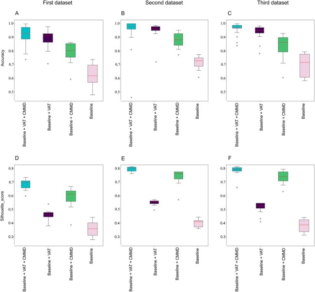
Box plots representing the impact of different loss functions on accuracy and batch effect mitigation based on the ablation study. Panels (A–C) show the model accuracies on the first, second, and third datasets, respectively. Panels (D–F) present the Silhouette score based on the first, second and third datasets, respectively. All panels present the outcome based on selecting 70% of the data as source domain randomly and selecting 30% of the data as target domain randomly and repeating training and testing 100 times. The line inside each box plot indicates the median of the outcome
Per panels D–F, the baseline model with both VAT and CMMD loss functions consistently provides the highest Silhouette score that indicates the highest alignment between pairwise clusters in different batches (mitigating batch effect). The baseline model with CMMD only consistently provides a better batch alignment compared to the baseline model with VAT only. The baseline model alone provides the lowest alignment consistently.
As such, all the loss functions impact the outcome; while VAT is critical in improving the accuracy, CMMD is critical in mitigating the batch effect and improving the alignment between pairwise clusters of different batches. The accuracy of the baseline model with VAT and CMMD loss functions on the first (Fig. 4A), second (Fig. 4B) and third (Fig. 4C) datasets were 92%, 97% and 97%, respectively.
Figure 4D–F show that CMMD impacts cell type alignments in first, second and third datasets substantially. The Silhouette score for the Baseline model with VAT and CMMD loss functions on the first (Fig. 4D), second (Fig. 4E) and third (Fig. 4F) datasets were about 0.70, 0.80 and 0.79%, respectively. These results reflect the impact of CMMD on mitigating the effect of batches.
The number of cells in clusters was not distributed normally based on Shapiro–Wilk normality test (see also Fig. 5B). We thus tested the correlation between the number of cells in clusters and their corresponding accuracy based on Kendall and Spearman (non-parametric correlation tests). The correlation coefficients were 0.06 and 0.09, and the P-values were 0.62 and 0.58, respectively. As such, there was no association between the number of cells and accuracy in different clusters.
Fig. 5.

Experiments on the first dataset. Panel (A) shows the accuracies of our model as well as some state-of-the-art cell type identification models where x-axis denotes different single batches as target domain and the rest of the other batches as source domain on the first dataset. Panel (B) shows cell counts in different batches on the first dataset
The number of transcripts (expressed in cells) in clusters was distributed normally based on Shapiro–Wilk normality test (P = 0.11). The correlation coefficient based on Pearson test was −0.06 with the P-value of 0.67. As such, there was no association between the number of genes in clusters and their respective accuracy.
Figure 5A illustrates the accuracies of our model compared with other models based on different batches of the first dataset. We selected one of the batches as the target domain and the other batches as the source domain and evaluated the accuracy of all models. Our model consistently outperformed the other models with a range of accuracy of [0.92–0.93]. Figure 5B shows the number of cell types in different batches of the first dataset.
The number of cells in each class (subtype) for all three datasets is shown in Supplementary Table S2. We performed three additional analyses to investigate the impact of different number of cells and genes on accuracy. Supplementary Figure S1A shows the impact of randomly selecting 25%, 50%, 75% and 100% of the cells in each class (cell type) on accuracy based on the first and second datasets while keeping the number of genes intact (2000 highly variable genes). The accuracy was compromised once the number of selected cells decreased significantly. Based on these data, over ∼50 single cells per cell types are minimally required in the source domain to reach an accuracy of ∼90%. Supplementary Figure S1B shows the impact of randomly selecting 25%, 50%, 75% and 100% of the genes in each class (cell type) on accuracy based on the first and second datasets while keeping the number of cells for each dataset intact. The classification accuracy was compromised once the number of selected genes decreased substantially. Supplementary Figure S2 shows a scenario in which we selected 1000, 1500, 2000, 2500 and 3000 top highly variable genes for the downstream analysis. The accuracy was compromised when we selected fewer than 2000 highly variable genes. We evaluated the accuracy level of our algorithm and several state-of-the-art single-cell models including CHETAH (De Kanter et al., 2019), CaSTLe (Lieberman et al., 2018), scPred (Alquicira-Hernandez et al., 2019), SingleR (Aran et al., 2019), SVM (Pedregosa et al., 2011) and KNN (Pedregosa et al., 2011), based on the first (Macosko et al., 2015), second (Rheaume et al., 2018) and third (Tran et al., 2019) datasets. We selected the default parameters for CHETAH, CaSTLe, scPred, SingleR which were recommended in the original papers. We used k = 30 for the KNN classifier and employed radial kernel function for the SVM classifier. Our proposed model achieved the classification accuracy of 92%, 97% and 97% (Tables 1–3, based on 70/30 split), the accuracy of the CHETAH model was 87%, 95% and 94%, the accuracy of the CaSTle model was 89%, 95% and 95%, the accuracy of the scPred model was 90%, 95% and 96%, the accuracy of the SingleR model was 91%, 96% and 96%, the accuracy of the SVM model was 90%, 95% and 96%, and finally, the accuracy of the KNN model was 86%, 93% and 92% on the first, second and third datasets, respectively.
The accuracy of the model based on three pancreas datasets from Baron mouse and Tabula Muris mouse (selected as source data) and Segerstolpe human (selected as target data) species was about 99% (see Supplementary Table S1). As this analysis was cross-dataset and cross-species, the proposed model was shown to be robust and dependable in dealing with real-world scenarios.
4 Discussion
In this article, we describe the development of a deep learning-based domain adaptation model for distinguishing different single retinal cell types and RGC subtypes from scRNA-seq data. We employed min–max loss, VAD loss, CMMD loss and a cross-entropy loss through both labeled source and unlabeled target datasets. We showed that our model achieved high accuracy in classifying a large number of retinal cell types (39 classes) and RGC subtypes (41 classes; including one non-RGC cells) and (45 classes). While heterogeneity among different batches in single-cell data poses a major challenge, our model consistently achieved high accuracies using one batch as source and other batches as target domain data.
Our proposed model could prove highly useful in the construction of cell atlases of various tissues, such as CNS neurons in the retina that are compromised by glaucoma, thus providing important insights into glaucoma pathogenesis (van Zyl et al., 2020). Transcriptome markers play a major role in gaining insight to cell types and their susceptibility and involvement in disease. However, as the scale of single-cell data increases, the conventional methods for cell identification become more challenging in terms of labor, resources and computational models. We have proposed a novel model that can learn transcriptomic patterns from a dataset with labeled cell types and then use the gained knowledge to identify cell types and subtypes of unseen datasets with large number of cells. The mean accuracy of our model (based on 70/30 split) in correctly identifying 39 retinal cell types was ∼92% while the accuracy in correctly recognizing 40 RGC subtypes (excluding the non-RGC class labeled C0) was ∼97% and the mean accuracy on the other 45 RGC subtypes was ∼97%, reflecting a high accuracy despite the existence of a large number of cell types. The proposed model could be readily used to identify retinal cell types and RGC subtypes based on scRNA-seq data for future ophthalmic studies.
We evaluated the accuracy and robustness of the model based on three independent datasets with large numbers of cells. The first dataset (M) included over 44 000 single retinal cells and the second dataset (R) included more than 6000 single RGCs, and the third dataset (T) contained over 35 000 single RGCs. The accuracy of the model for each of the 39 retinal cell types and subtypes ranged between 76% and 85%, based on using cells in one batch as the source and cells in another batch as target (Fig. 2A–G). Several reasons could explain obtaining lower accuracy based on batches compared to using all merged cells. First, scRNA-seq data are prone to inconsistent amplification during library preparation when different batches are generated (Li and Li, 2018). Cell types and their proportions may also vary substantially in different batches (Liu et al., 2018). In addition, cell extraction, isolation, amplification and sequencing may also vary under different conditions and batch preparation. Collectively, these may lead to heterogeneity in single cells in different batches, which represent a major challenge in scRNA-seq data analysis studies. In addition to batch effect, the accuracy of the proposed model may also have been impacted by the significantly fewer cells in each batch compared to the merged subset. Nevertheless, the mean accuracy of the model based on different batches was consistently over 80% with only one exception (models based on Batch B1 as target, generated lower accuracy; see Fig. 2B–G). When we merged all batches and used 70% of the cells as the source domain and the remaining 30% cells as the target domain, the classification accuracy improved to ∼92% (see Table 1).
The model was more accurate on single RGCs in the second dataset and provided a mean accuracy of about 97% in classifying different RGC subtypes. In fact, there are only 40 RGC subtypes and class 0 is composed of all non-RGC cells that have somehow entered the analysis in the experimental workflow (outliers). The model’s accuracy on all RGC subtypes was consistently over 90% (see Table 2).
Additionally, the accuracy of the model on single RGCs in the third dataset with 45 different RGC subtypes was ∼97% (Table 3). The higher accuracy of the model based on the second and third datasets (with single RGCs), compared to the first dataset (with single retinal cells), could be explained by the fact that all single RGCs in the first dataset were collected based on one experiment, and all single RGCs in the third dataset were collected based on only three batches. However, the first dataset included seven different batches. Therefore, we expect that the second and third datasets have lower heterogeneity compared to the first dataset. This can be supported by the fact that cells in Batch B1 of the first dataset have lower quality compared to the cells in the rest of batches (Fig. 2B–G; the accuracy is consistently lower when Batch B1 is tested). The accuracy of other models based on the B1 batch is also lower compared to the other batches (Fig. 5A). Moreover, this batch has a significantly smaller number of cells compared to other batches (Fig. 5B).
To better evaluate the accuracy level of our algorithm, we compared our model against several state-of-the-art cell type identification models including CHETAH (De Kanter et al., 2019), CaSTLe (Lieberman et al., 2018), scPred (Alquicira-Hernandez et al., 2019), SingleR (Daniszewski et al., 2018), SVM (Pedregosa et al., 2011) and KNN (Pedregosa et al., 2011). We evaluated these models based on the first (Macosko et al., 2015), second (Rheaume et al., 2018) and third (Tran et al., 2019) datasets, and consistently obtained higher performance. Additionally, we accessed three datasets based on pancreas tissues from different species generated by different platforms. Specifically, we used the Baron mouse and the Tabula Muris mouse cell datasets as source domain data, and the Segerstolpe human cell dataset as the target domain data. We obtained an accuracy of 99% (Supplementary Table S1) in detecting correct class based on this cross-data analysis reflecting the fact that the model is generalizable to unseen datasets.
Our proposed model has several advantages. First, it can be readily used to identify retinal cell types and RGC subtypes based on transcriptome profiles. It is also reasonably resistant to batch effect. However, it requires labels for the source domain data, and thus may seem not applicable to scenarios for which labeled data are not available. To mitigate this issue, we can select a subset of unlabeled data and perform a clustering approach (e.g. based on Seurat package) to identify cell types with high membership likelihood. We can then use this labeled subset as the source and train the proposed model to identify the labels of the rest of the data. It is worth mentioning that many scRNA-seq datasets are becoming publicly available to the community which could, in turn, be used as source domain data for our algorithm. Second, the proposed model was not evaluated based on data from two different labs. None of the three vision-based datasets that we experimented was appropriate for cross-data test because they had at most three clusters in common (first and second datasets). The second and third datasets were not appropriate for this experiment as well as the second dataset included RGCs from pre-eye-opening (5 days postnatal) while the third dataset included eyes from adult mice aged 6–20 weeks. The clusters and transcriptome were different as visual experience (aging) shapes the maturation of retinal circuitry and development process typically triggers more RGC subtypes (Tian and Copenhagen, 2003). Cell extraction, isolation, amplification (overall conditions) and sequencing varies for different batches. Therefore, cross-batch could be a subset of cross-data experiment. Future studies may investigate the impact of cross-data on the model. However, we performed cross-batch experiments based on the first and third datasets.
In conclusion, we developed a deep-learning-based domain adaptation model to detect retinal cell types and RGC subtypes from transcriptome profiles. The model was highly accurate in detecting correct RGC subtypes and was resistant to the batch effect. Further validation of our model holds promise for future studies to identify transcriptome profiles of RGCs and other cells involved in glaucoma to shed light on molecular aspects of glaucoma pathogenesis.
Funding
This work was supported by the Bright Focus Foundation, NIH EY033005, and a Challenge Grant from Research to Prevent Blindness (RPB). The funders had no role in study design, data collection and analysis, decision to publish or preparation of the manuscript.
Conflict of Interest: none declared.
Supplementary Material
Contributor Information
Yeganeh Madadi, Department of Ophthalmology, University of Tennessee Health Science Center, Memphis, TN, USA; University of Tehran, Tehran, Iran.
Jian Sun, Department of Ophthalmology, University of Tennessee Health Science Center, Memphis, TN, USA.
Hao Chen, Department of Pharmacology, Addiction Science and Toxicology, University of Tennessee Health Science Center, Memphis, TN, USA.
Robert Williams, Department of Genetics and Informatics, University of Tennessee Health Science Center, Memphis, TN, USA.
Siamak Yousefi, Department of Ophthalmology, University of Tennessee Health Science Center, Memphis, TN, USA; Department of Genetics and Informatics, University of Tennessee Health Science Center, Memphis, TN, USA.
References
- Alquicira-Hernandez J. et al. (2019) scPred: accurate supervised method for cell-type classification from single-cell RNA-seq data. Genome Biol., 20, 264. [DOI] [PMC free article] [PubMed] [Google Scholar]
- Aran D. et al. (2019) Reference-based analysis of lung single-cell sequencing reveals a transitional profibrotic macrophage. Nat. Immunol., 20, 163–172. [DOI] [PMC free article] [PubMed] [Google Scholar]
- Butler A. et al. (2018) Integrating single-cell transcriptomic data across different conditions, technologies, and species. Nat. Biotechnol., 36, 411–420. [DOI] [PMC free article] [PubMed] [Google Scholar]
- Cao Z. et al. (2020) Searching large-scale scRNA-seq databases via unbiased cell embedding with cell BLAST. Nat. Commun., 11, 1–13. [DOI] [PMC free article] [PubMed] [Google Scholar]
- Chalupa L.M., Williams R. W. (2008) Eye, Retina, and Visual System of the Mouse. Oxford University Press; MIT Press, Cambridge. [Google Scholar]
- Chen L. et al. (2020) SeqVAT: Virtual adversarial training for semi-supervised sequence labeling. Paper presented at the Proceedings of the 58th Annual Meeting of the Association for Computational Linguistics.
- Cui S. et al. (2020) Towards discriminability and diversity: Batch nuclear-norm maximization under label insufficient situations. Paper presented at the Proceedings of the IEEE/CVF Conference on Computer Vision and Pattern Recognition.
- Daniszewski M. et al. (2018) Single cell RNA sequencing of stem cell-derived retinal ganglion cells. Sci. Data, 5, 1–9. [DOI] [PMC free article] [PubMed] [Google Scholar]
- De Kanter J.K. et al. (2019) CHETAH: a selective, hierarchical cell type identification method for single-cell RNA sequencing. Nucleic Acids Res., 47, e95. [DOI] [PMC free article] [PubMed] [Google Scholar]
- Ding J., Regev A. (2021) Deep generative model embedding of single-cell RNA-Seq profiles on hyperspheres and hyperbolic spaces. Nat. Commun., 12, 1–17. [DOI] [PMC free article] [PubMed] [Google Scholar]
- Ganin Y., Lempitsky V. (2015) Unsupervised domain adaptation by backpropagation. Paper Presented at the International Conference on Machine Learning, Lille, France.
- Geisert E.E., Williams R.W. (2008) The mouse eye transcriptome: cellular signatures, molecular networks, and candidate genes for human disease. In: Chalupa,L.M. and Williams,R.W. (eds) Eye, Retina, and Visual System of the Mouse. MIT Press, Cambridge, pp. 659–674. [Google Scholar]
- Haghverdi L. et al. (2018) Batch effects in single-cell RNA-sequencing data are corrected by matching mutual nearest neighbors. Nat. Biotechnol., 36, 421–427. [DOI] [PMC free article] [PubMed] [Google Scholar]
- Johnson T.S. et al. (2019) LAmbDA: label ambiguous domain adaptation dataset integration reduces batch effects and improves subtype detection. Bioinformatics, 35, 4696–4706. [DOI] [PMC free article] [PubMed] [Google Scholar]
- Kang G. et al. (2019) Contrastive adaptation network for unsupervised domain adaptation. Paper Presented at the Proceedings of the IEEE/CVF Conference on Computer Vision and Pattern Recognition, Long Beach, California.
- Łabaj P.P., Kreil D.P. (2016) Sensitivity, specificity, and reproducibility of RNA-Seq differential expression calls. Biol. Direct, 11, 1–12. [DOI] [PMC free article] [PubMed] [Google Scholar]
- Levin L.A. (2005) Retinal ganglion cells and supporting elements in culture. J Glaucoma, 14, 305–307. [DOI] [PubMed] [Google Scholar]
- Li J. et al. (2020) Maximum density divergence for domain adaptation. IEEE Trans. Pattern Anal. Mach. Intell., 43, 3918–3930. [DOI] [PubMed] [Google Scholar]
- Li W.V., Li J.J. (2018) An accurate and robust imputation method scImpute for single-cell RNA-seq data. Nat. Commun., 9, 997. [DOI] [PMC free article] [PubMed] [Google Scholar]
- Lieberman Y. et al. (2018) CaSTLe—classification of single cells by transfer learning: harnessing the power of publicly available single cell RNA sequencing experiments to annotate new experiments. PLoS One, 13, e0205499. [DOI] [PMC free article] [PubMed] [Google Scholar]
- Liu Q. et al. (2018) Quantitative assessment of cell population diversity in single-cell landscapes. PLoS Biol., 16, e2006687. [DOI] [PMC free article] [PubMed] [Google Scholar]
- Lopez R. et al. (2018) Deep generative modeling for single-cell transcriptomics. Nat. Methods, 15, 1053–1058. [DOI] [PMC free article] [PubMed] [Google Scholar]
- Lukowski S.W. et al. (2019) A single-cell transcriptome atlas of the adult human retina. EMBO J., 38, e100811. [DOI] [PMC free article] [PubMed] [Google Scholar]
- Macosko E.Z. et al. (2015) Highly parallel genome-wide expression profiling of individual cells using nanoliter droplets. Cell, 161, 1202–1214. [DOI] [PMC free article] [PubMed] [Google Scholar]
- Madadi Y. et al. (2020) Deep visual unsupervised domain adaptation for classification tasks: a survey. IET Image Process, 14, 3283–3299. [Google Scholar]
- Pedregosa F. et al. (2011) Scikit-learn: machine learning in python. J. Mach. Learn. Res., 12, 2825–2830. [Google Scholar]
- Rheaume B.A. et al. (2018) Single cell transcriptome profiling of retinal ganglion cells identifies cellular subtypes. Nat. Commun., 9, 2759. [DOI] [PMC free article] [PubMed] [Google Scholar]
- Rokicki W. et al. (2007) Retinal ganglion cells death in glaucoma–mechanism and potential treatment. Part II. Klin. Oczna., 109, 353–355. [PubMed] [Google Scholar]
- Seung H.S., Sümbül U. (2014) Neuronal cell types and connectivity: lessons from the retina. Neuron, 83, 1262–1272. [DOI] [PMC free article] [PubMed] [Google Scholar]
- Stuart T. et al. (2019) Comprehensive integration of single-cell data. Cell, 177, 1888–1902.e21. [DOI] [PMC free article] [PubMed] [Google Scholar]
- Tanabe Y., Jessell T.M. (1996) Diversity and pattern in the developing spinal cord. Science, 274, 1115–1123. [DOI] [PubMed] [Google Scholar]
- Tian N., Copenhagen D.R. (2003) Visual stimulation is required for refinement of on and off pathways in postnatal retina. Neuron, 39, 85–96. [DOI] [PubMed] [Google Scholar]
- Tran N.M. et al. (2019) Single-cell profiles of retinal ganglion cells differing in resilience to injury reveal neuroprotective genes. Neuron, 104, 1039–1055.e12. [DOI] [PMC free article] [PubMed] [Google Scholar]
- van Zyl T. et al. (2020) Cell atlas of aqueous humor outflow pathways in eyes of humans and four model species provides insight into glaucoma pathogenesis. Proc. Natl. Acad Sci. USA, 117, 10339–10349. [DOI] [PMC free article] [PubMed] [Google Scholar]
- Wang T. et al. (2019) Bermuda: a novel deep transfer learning method for single-cell RNA sequencing batch correction reveals hidden high-resolution cellular subtypes. Genome Biol., 20, 165. [DOI] [PMC free article] [PubMed] [Google Scholar]
- Williams R.W. et al. (1993) Rapid evolution of the visual system: a cellular assay of the retina and dorsal lateral geniculate nucleus of the Spanish wildcat and the domestic cat. J. Neurosci., 13, 208–228. [DOI] [PMC free article] [PubMed] [Google Scholar]
- Williams R.W., Moody S.A. (2003) Developmental and genetic control of cell number in the retina. In: Chalupa L.M., Werner J.S. (eds.) The Visual Neurosciences. MIT Press, Cambridge, pp. 65–78. [Google Scholar]
- Zareparsi S. et al. (2004) Seeing the unseen: microarray-based gene expression profiling in vision. Invest. Ophthalmol. Vis. Sci., 45, 2457–2462. [DOI] [PubMed] [Google Scholar]
- Zhu Y. et al. (2019) Multi-representation adaptation network for cross-domain image classification. Neural Netw., 119, 214–221. [DOI] [PubMed] [Google Scholar]
Associated Data
This section collects any data citations, data availability statements, or supplementary materials included in this article.