

Abstract
Proteins are key components in many processes in living cells, and physical interactions with other proteins and nucleic acids often form key parts of their functions. In many cases, large flexibility of proteins as they interact is key to their function. To understand the mechanisms of these processes, it is necessary to consider the 3D structures of such protein complexes. When such structures are not yet experimentally determined, protein docking has long been present to computationally generate useful structure models. However, protein docking has long had the limitation that the consideration of flexibility is usually limited to very small movements or very small structures. Methods have been developed which handle minor flexibility via normal mode or other structure sampling, but new methods are required to model ordered proteins which undergo large-scale conformational changes to elucidate their function at the molecular level. Here, we present Flex-LZerD, a framework for docking such complexes. Via partial assembly multidomain docking and an iterative normal mode analysis admitting curvilinear motions, we demonstrate the ability to model the assembly of a variety of protein-protein and protein-nucleic acid complexes.
Keywords: protein-protein docking, protein-nucleic acid docking, nucleic acid docking, flexible docking, flexible assembly
INTRODUCTION
Protein-protein interactions are fundamental to many biological processes in living cells. To understand in detail the mechanisms of these processes, modeling the 3D structures of their associated protein complexes is a critical step. While protein complex structures are steadily being determined by experiment and deposited in the Protein Data Bank (PDB) [1], experiments are costly both in time and expense. Moreover, structures of protein complexes are often extremely difficult to determine by experiments. Thus, when a protein complex structure has not yet been experimentally determined, computational tools can be used to construct atomic models [2]. A so-called protein docking program can take component proteins, called subunits, as input and assemble them into atomic models of the protein complex. Many general protein docking methods and specialized versions thereof have been publicly released, such as ZDOCK [3], HADDOCK [4], ClusPro [5], RosettaDock [6], HEX [7], SwarmDock [8], and ATTRACT [9]. Even protein structure prediction methods like AlphaFold [10] have been tweaked to be able to output multimeric structures [11]. The rigid-body docking method LZerD [12–15] in particular has been consistently ranked highly in the server category in CAPRI [16, 17], the blind communitywide assessment of protein docking methods.
Often confounding to computational complex modeling is the fact that proteins are flexible molecules. Even with state-of-the-art conformational sampling techniques, existing docking methods struggle to handle substantial conformational changes beyond roughly 2 Å RMSD [18–20]. Large scale conformational changes near and above 10 Å RMSD, though well above 2 Å RMSD and thus difficult to model, are quite common, and are often related to protein function [21–27]. For example, in many cellular processes, calmodulin, ubiquitous in eukaryotes, undergoes such a conformational change when it binds to its various target proteins, and its flexibility facilitates recognition of a comparatively large number of targets in tandem with increases in Ca2+ ion concentration [28]. In the case of the nuclear import cycle, a crucial step is the release of the importing-beta-binding domain of importin-alpha from importin-beta by GTPase Ran. The binding of GTPase Ran to importin-beta induces a large-scale change in the helical conformation of importin-beta, allosterically inducing the importin subunits to dissociate [29]. It is then clear that techniques capable of modeling such large conformational changes have the potential to elucidate many cellular processes in many cellular contexts.
Computational techniques have been developed which quantitatively predict the location, nature, or degree of conformational change a given protein might undergo [30–33], including as part of complex formation [34]. While existing assembly methods generally struggle with a few angstroms root mean squared deviation (RMSD) of conformational change [18], experimentalists often observe far more drastic conformational changes [21–27]. There are many ways to consider lesser flexibility. The implicitly soft surface representation of LZerD [12, 13] can handle side chain flexibility. When the backbone must be moved, it can be sampled explicitly e.g. by ClustENM [20, 35] with normal modes, by CABS-Dock [36] or RosettaDock [37] with Monte Carlo simulation, or by ATTRACT with molecular dynamics [38, 39]. Many explicit sampling methods require cross-docking, which necessitates either precise sampling or fast sample docking to prevent intractable computation times [40, 41]. At the extreme end of the flexibility spectrum, intrinsically disordered proteins and protein regions can currently be docked by IDP-LZerD [42–44], even at ligand disordered region sizes of 69 residues. However, IDP-LZerD is specific for docking a disordered protein with no structured domains and relies on docking and knitting together necessarily small peptide fragments to a receptor protein and is thus not suitable for assembling complexes with large, ordered ligand domains. Despite substantial advancements, existing protein docking methods cannot generally model large-scale conformational changes of ordered ligand proteins. Current methods can handle some lesser flexibility [20], but cannot seem to break a barrier at larger RMSDs of conformational change. In the regime of conformational change ≥10.0 Å RMSD even with coherent domains, current methods are simply not adequate.
In this work, we target this ≥10.0 Å RMSD coherent regime, and describe a new method called Flex-LZerD. Flex-LZerD is comprised of a novel method for normal mode-based flexible fitting of an initial structure to docked partial structure fragments, here domains, and a method for selecting these partial docked structure domains. This restriction of the expensive rigid-body docking to the initial stage circumvents the cross-docking problem and renders the large-scale flexible docking tractable. Previous work by Karaca and Bonvin showed multidomain docking to be a promising route, but did not handle large gaps and mainly considered benchmark targets well below the 10.0 Å RMSD regime [45]. The novel fitting by iterative projection along residue-level rigid block normal modes to the docked domains and geometry minimization, at multiple levels with and without the receptor structure, then yields all-atom models in the new putative bound states. Past work in loop modeling has developed methods capable of modeling typically up to 12-residue-long gaps in a protein structure where both endpoints are known [46]. However, our benchmark in this work contains domain pairs with dozens to hundreds of unmodeled residues. These gaps are well outside the range of loop modeling but are handled in this context by the flexible fitting. We will directly show that the examined flexibility regime is inaccessible to rigid-body docking, that deep learning methods like AlphaFold do not currently handle such structures which are observed in different conformations, that flexible fitting is capable of modeling the conformational differences within the regime, and that Flex-LZerD as a whole is capable of flexibly assembling ligand and receptor proteins and nucleic acids into complex models. Interactions of both DNA and RNA with proteins are handled in this framework. Flex-LZerD yielded acceptable models within the top 10 models for 5 of the 9 unbound docking cases where the receptor structure used was also unbound, according to the CAPRI criteria. On a broader unbound/bound benchmark set where the receptor structure was in its bound form, Flex-LZerD likewise yielded acceptable models within the top 10 models for 17 of 23 total targets. These successes break down into 9 of 15 protein-protein complexes and 8 of 8 protein-nucleic acid complexes modeled to acceptable quality. The Flex-LZerD flexible fitting code is available from https://github.com/kiharalab/Flex-LZerD.
RESULTS AND DISCUSSION
Overview of Flex-LZerD
The docking procedure of Flex-LZerD is based on observation that often the assembly of complexes involving large-scale conformational change is established by interactions of individual almost rigid domains of the ligand protein with the receptor. Flex-LZerD builds full-complex models by independently docking domains extracted from a ligand structure, and then using an iterative fitting procedure to dock the complete ligand structure. The overall steps of this procedure are shown in Figure 1.
Figure 1.
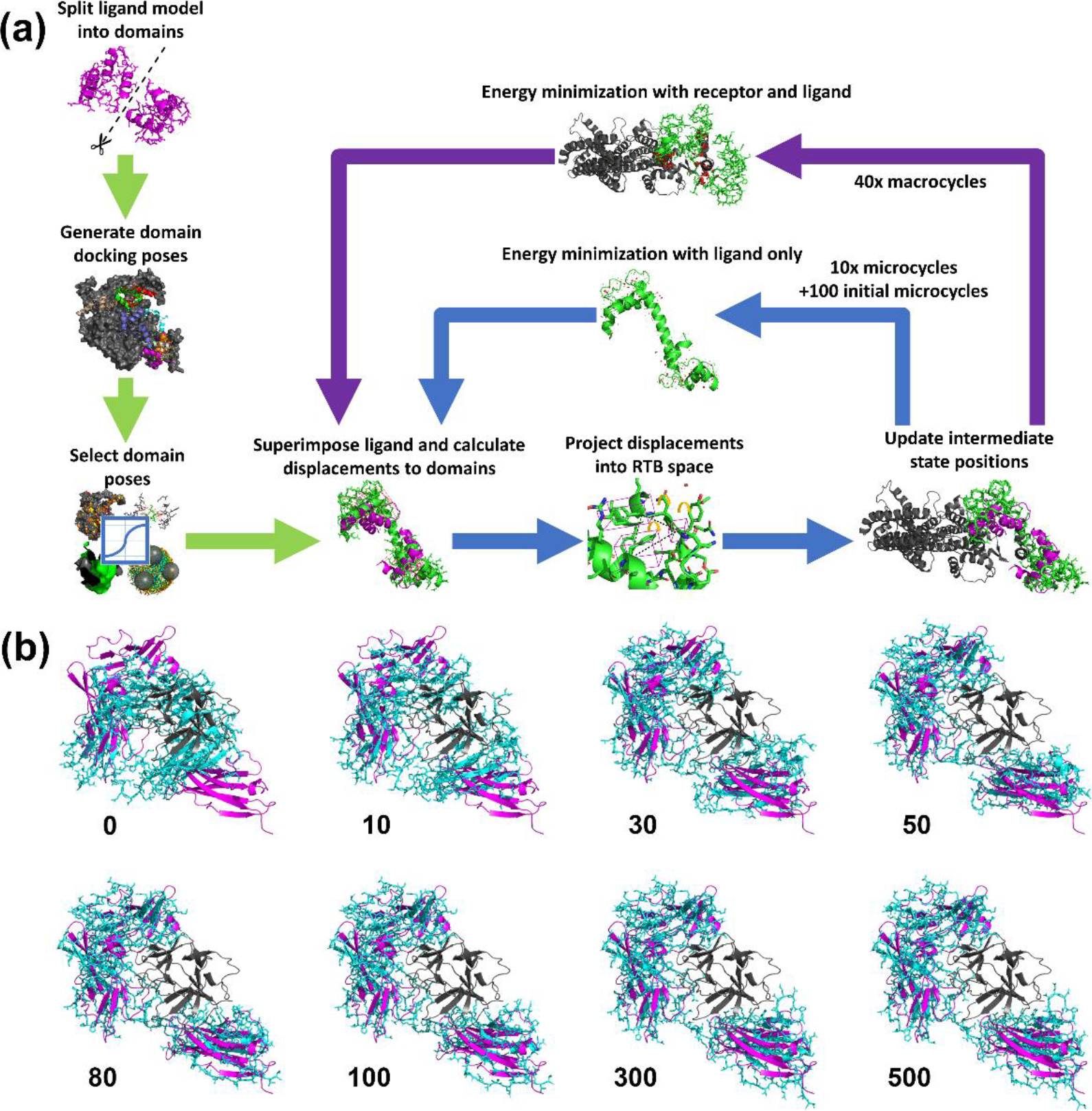
(a) Overall flow of the Flex-LZerD method. Green: the initial stage of the pipeline, which yields partially assembled complex models. Two domains are extracted from the ligand, the domains are docked to the receptor, and domain poses are selected via a consensus scoring function. Blue: the microcycle loop of the pipeline, where atom coordinates are updated according to normal mode displacements and energy minimization of the ligand. The energy minimization using PHENIX takes into account bonds and steric effects, but not long-range interactions. Purple: the macrocycle loop of the pipeline, where atom coordinates are updated according to an otherwise identical energy minimization of the ligand in the presence of the receptor. (b) A selection of frames from a flexible fitting run of target Interleukin-1 receptor type 1 (PDB 1ITB). Gray: the receptor structure. Magenta: the docked domain models being fitted to. Cyan: the unbound ligand model being deformed. Frame 0 is simply the input ligand unbound structure superimposed to the docked domain models. The bulk of the conformational change was modeled early on while the domain displacement vectors were large. After iteration 100 when the receptor was included in the geometry minimization, the fit adjusted to conform to the receptor structure. Frame 500 is the output model for this docked domain model pair, which has an I-RMSD of 3.9 Å, an L-RMSD of 4.0 Å, and an fnat of 0.29.
The first step is to extract domains from the input ligand structure. In cases where the ligand has clear globular domains connected by loops, the globular domains can be obviously split. In many cases, such as the interleukin-1 receptor, a flexible loop appropriate to cut can be indicated by a local peak in the flexibility predict by FlexPred [30, 31]. A flexible loop that links globular domains typically has a predicted fluctuation of over 3 Å, which is higher than the remainder of the protein chain. Domains were also selected based on biological knowledge, such as EF-hand domains in calmodulin, which are exceptionally well-known in the literature [47] or HEAT repeats [48] in importin-beta. There is no restricted maximum sequence distance between the domains. Details of the domain extraction for each benchmark target are provided in Supplemental Table S1. Once the domains were specified, they were subsequently docked separately using LZerD [12, 49], a shape complementarity-based rigid-body docking which uses a soft representation of the molecular surface to achieve tolerance to some small conformational changes. After truncating the number of outputs to 50,000 as is usual with LZerD [13], the generated domain docking poses were clustered at 4.0 Å RMSD to remove redundancy.
In the next stage, to select domain poses we used a combined scoring function generalized from methods used in the scoring of IDP-LZerD [42], which incorporates both statistical knowledge-based scoring functions and model consensus features. We incorporated the knowledge-based scoring functions used in ranksum [13, 50, 51], which has performed well in recent rounds of the Critical Assessment of Prediction of Interactions (CAPRI) [16, 17, 52–54], a blind communitywide experiment evaluating protein complex modeling methods. For each domain, the top 100 docked models were selected by the combined score.
Once the 100 models are selected for each domain, we subsequently considered them pairwise and flexibly deformed them to dock against the receptor via iterations of normal mode analysis and energy minimization. Thus, we consider 100*100 = 10,000 models. Herein lies the core novelty of Flex-LZerD. Prior to normal mode calculation, the ligand structure was centered to minimize the RMSD to the domain pose pair, corresponding to the superimposition step in Figure 1. This superimposition step serves only to center and orient the starting structure to remove the need to consider mathematically degenerate normal modes and does not itself deform the structure—even in a protein-protein complex where the domains were docked perfectly matching the native structure, the superimposed ligand would still have an unchanged RMSD to the native structure, i.e. ≥ 10.0 Å with our benchmark set. We calculated modes in a reduced representation via the rotations and translations of blocks (RTB) [55] method, detailed in “Rotations and translations of blocks” in “Materials and Methods”. RTB allowed us to define blocks, here synonymous with residues, which were considered as rigid bodies during normal mode calculation. Neglecting the internal flexibility of individual residues discouraged nonphysical distortions and reduced the computational cost of each normal mode calculation, which can otherwise be problematic with large structures [33]. Using the 20 lowest-frequency nondegenerate normal modes, we displaced atom coordinates of the ligand in straight lines in small increments of collective motion to update the fitted state. A cutoff of 20 modes is commonly used in the context of protein complexes [34, 56] and provides reasonable confidence that even especially large ligands will be reasonably well characterized. These normal modes only allow displacement in straight lines, even when adding multiple normal modes simultaneously. To accomplish curvilinear motion, modes were restricted to small amplitude motion after being weighted by the projection of the displacements that would transform the ligand structure to exactly match the docked domains, attenuated by a factor of 0.05, corresponding to the projection step in Figure 1. Then, after such a small displacement was applied, corresponding to the update step in Figure 1, the ligand was re-centered and the normal modes were re-calculated, corresponding biophysically to the fact that the intramolecular interactions have now changed somewhat. Naturally, no exact displacement can be blindly calculated here for regions of the ligand, such as regions linking the domains, which are not modeled in the domain docking. Instead, these displacements were imputed from the mode amplitudes obtained from the aforementioned projection considering only the regions modeled in domain docking. With this imputation, displacements are obtained for all atoms in the input ligand structure. Thus, using many line segments, curvilinear motion was accomplished, modeling the transit between states. After each of up to 500 fitting iterations, or fewer if a 4-hour time limit is exceeded, the structure was processed using the geometry minimization library (in Python, “mmtbx.refinement.geometry_minimization”) from the PHENIX package [57] to preserve the physicality of the model. This process is detailed in “Minimization of geometric restraints” in “Materials and Methods”. Despite the small amplitudes applied, properties like covalent bond lengths, Van der Waals strain, and torsion angles can be distorted over many unchecked iterations. Even the peptide bond can be distorted by the normal mode displacement, so this step was critical to producing protein-like output. Subsequently, to incorporate information from the receptor structure into the geometry minimization, both the receptor and ligand structures were included every 10 iterations after 100 initial microcycles of fitting, corresponding to the 40 macrocycles shown in Figure 1 (outer cycle). On other iterations, only the ligand structure was minimized, corresponding to the microcycles shown in Figure 1 (inner cycle). The fitted model set was scored again by the combined scoring function.
To illustrate the progression of the fitting procedure, a series of frames from a fitting run from benchmark target 1ITB are shown in Figure 1b, with a full video of the entire fitting available as Supplemental Video S1. Each subpanel of Figure 1b shows a frame labeled by the frame number. Frame 0 is the initial input structure superimposed to the docked domain poses. At this stage, the unbound ligand structure (cyan) was in essence merely centered without yet considering flexibility, with an I-RMSD of 10.3 Å, an L-RMSD of 5.9 Å, and an fnat of 0.03. At frame 10, the ligand began to open somewhat, with an I-RMSD of 9.0 Å. By frame 30, the ligand was almost fully open, with an I-RMSD of 8.4 Å. At frame 50, the C-terminal end of the ligand, which is the bottom domain in Figure 1b, was rotating in bulk towards the orientation of the docked C-terminal domain, with an I-RMSD of 7.7 Å. At frame 80, the rotation was nearly complete, with an I-RMSD of 5.6 Å, an L-RMSD of 4.2 Å, and an fnat of 0.29. The rotation was essentially complete at frame 100, with an I-RMSD of 4.7 Å, but the interface structure does not yet sterically complement the receptor. By frame 300, the ligand now fit around the receptor, and the fitting has essentially plateaued, with an I-RMSD of 3.8 Å. The ligand reaches its final fitted pose accommodating the receptor at frame 500, with an I-RMSD of 3.9 Å, an L-RMSD of 4.0 Å, and an fnat of 0.29.
Overall Docking Results
We benchmarked Flex-LZerD on a nonredundant set of 23 targets. Of these, 15 are protein-protein interactions and 8 are protein-nucleic acid interactions. Potential targets were found by searching PDB for complex structures with corresponding unbound ligands, where the bound and unbound ligand structures differed by at least 10.0 Å RMSD for protein receptors and 7.0 Å RMSD for nucleic acid receptors. Candidates were then individually screened, including to select for targets where the 10.0 Å conformational difference was due to large scale changes in the ligand protein and not, for example, due to differently packed tails or domain swapping. The construction process is detailed in “Dataset construction” in “Materials and Methods”. We note that this dataset is aimed for complexes with a ligand protein that undergoes a large conformational change and thus different from a general docking benchmark dataset such as the ZDOCK dataset [58]. ZDOCK benchmark 5.5 has 271 targets, pairs of bound and unbound conformations. The average RMSD between bound and unbound an RMSD of 1.7 Å with the minimum and the maximum RMSD values of 0.0 Å and 32.1 Å, respectively. There are 9 targets in ZDOCK that have over 10 Å difference between bound and unbound, which are in the scope of the current work, and indeed all of them were either already used in our dataset or redundant with our dataset. Specifically, 1IRA, 1Y64, 1ZLI, 1H1V are included in our training set, and 5C7X, 6B0S, 5WUX, 4FQI, and 1BGX, are all immunoglobulin and redundant with immunoglobulin, 1DCL, in our dataset.
To evaluate models, we adopted the CAPRI criteria [17], where models are graded according to their interface RMSD (I-RMSD), which considers only interface backbone atoms, their ligand RMSD (L-RMSD), which considers the RMSD for one subunit when the other subunit is superimposed, and their fraction of native contacts (fnat), which considers the number of residue pairs in contact in the native structure that are also in contact in the model. Past work done on modeling of disordered proteins, which can be considered as the most flexible protein docking context, has considered an I-RMSD threshold of 6.0 Å to indicate successful fragment docking, which incorporates a tolerance for interface flexibility while still requiring the presence of native interactions at the protein-protein interface [42]. However, in the context of multidomain docking [45] and flexible fitting for large scale conformational change, the standard CAPRI I-RMSD, L-RMSD, and fnat thresholds of 4.0 Å, 10.0 Å, and 0.10 still capture the quality of docking results, with models exhibiting I-RMSDs between 4.0 Å and 6.0 Å often still satisfying the standard L-RMSD threshold.
The docking results of individual targets are summarized in Table 2. Before examining actual modeling results, we first discuss results in the Flex(ible)-fitting-to-native column in Table 2, where for each target the unbound ligand was superimposed to the bound ligand in its native structure with the receptor and put through the flexible fitting procedure. This experiment examines how the proposed flexible fitting protocol performs in the best-case scenario where two domains of a target are placed in the correct pose. For all but one case (2F23), the Flex-LZerD protocol was able to produce models of CAPRI-acceptable quality. For 16 cases (69.6%), the resulting I-RMSD was less than 3.0 Å. In the case of 2F23, an acceptable quality model was not yielded mainly due to a narrow binding site of the receptor (RNA polymerase), which caused steric clashes during the fitting process and made it difficult to fit the ligand (GreA factor homolog 1) to the correct pose. Overall, the results demonstrate that the protocol has ability to construct reasonably accurate models for the targets that need to consider the extreme flexibility of ligands.
Table 2.
Docking performance of individual targets. Targets are identified by their ligand PDB IDs. “/” indicates that the two numbers given are for the first and second domains, respectively. Domain hits, the number of CAPRI-acceptable quality domains within the top 100 by the combined scoring function. Numbers given in parentheses indicate models which did not meet the CAPRI-acceptable quality criteria. (n/a) indicates that the method would not take the target as input, i.e. because AlphaFold does not handle nucleic acids, or that an unbound structure was not available for comparison. (error) indicates that the method accepted the input but crashed. Flexible-fitting-to-native results are for the single output model generated when performing flexible fitting of the unbound structure directly to the bound native structure. Rigid-body LZerD results show the best I-RMSD in the entire rigid-body LZerD pipeline output set using the unbound ligand conformation, typically tens of thousands of models. AlphaFold results are out of the 5 models generated by AlphaFold v2.1.0 by default.
| Domain level |
Complex level (I-RMSD, Å) |
AlphaFold (I-RMSD, Å) |
||||||||||
|---|---|---|---|---|---|---|---|---|---|---|---|---|
| Ligand PDB | CAPRI-acceptablehits | Best fnat in top10 | Best I-RMSD in top10 (Å) | Best L-RMSD in top10 (Å) | Flex-fitting-to-native | Rigid-body LZerD | Top-scored | Best in top10 | Best in All | Unbound best in top 10 | Monomer with linker | Multimer |
|
|
|
|||||||||||
| 1CLL | 3/3 | 0.24/0.11 | 1.72/2.86 | 3.55/6.22 | 1.95 | (11.39) | 4.70 | 4.70 | 4.48 | n/a | (19.67) | 2.51 |
| 1G0Y | 1/4 | 0.14/0.39 | 3.62/1.57 | 8.59/3.74 | 3.06 | (14.10) | 3.89 | 3.89 | 3.89 | 3.95 | (16.65) | 1.50 |
| 3ND2 | 6/1 | 0.38/0.21 | 0.60/2.19 | 1.17/4.20 | 1.62 | (9.98) | 2.88 | 2.73 | 2.47 | 4.76 | 3.24 | 2.18 |
| 2F23 | 0/0 | 0.04/0.01 | 4.25/6.21 | 10.23/22.66 | (7.24) | (8.73) | (17.20) | (15.97) | (6.56) | n/a | (error) | (error) |
| 6D66 | 2/5 | 0.23/0.21 | 3.37/3.25 | 9.96/7.45 | 8.62 | (8.78) | 6.96 | (6.89) | 6.42 | n/a | (15.82) | (20.85) |
| 2MCG | 4/4 | 0.30/0.33 | 0.99/1.89 | 1.83/4.04 | 1.76 | (9.30) | 2.97 | 2.64 | 2.64 | 3.98 | 2.96 | 3.46 |
| 1UFK | 3/2 | 0.48/0.15 | 1.08/3.60 | 2.40/11.17 | 1.45 | (9.87) | 4.88 | 4.79 | 4.79 | 5.71 | 5.06 | 1.53 |
| 4TRG(B)a) | 2/0 | 0.18/0.09 | 2.23/4.15 | 6.28/10.68 | 1.81 | (10.80) | (7.06) | (7.04) | (6.44) | (7.84) | (14.06) | (17.46) |
| 4TRG(C)a) | 2/0 | 0.43/0.06 | 1.72/4.32 | 6.16/10.20 | 1.97 | (9.28) | (7.19) | (7.19) | (7.17) | (8.22) | (8.57) | (24.93) |
| 3OJW | 1/3 | 0.12/0.62 | 3.34/1.60 | 17.66/5.82 | 2.71 | (8.27) | (8.73) | (7.19) | (6.80) | (8.50) | (16.56) | 6.18 |
| 1E0O | 3/3 | 0.17/0.36 | 2.86/1.69 | 16.20/2.62 | 5.60 | (8.11) | 4.43 | 4.43 | 4.16 | 4.51 | (9.40) | 0.70 |
| 4KSE | 0/0 | 0.02/0.08 | 7.20/2.38 | 18.44/7.87 | 1.73 | (13.23) | (24.87) | (20.86) | (18.58) | n/a | (19.16) | (21.44) |
| 2OK5 | 2/1 | 0.21/0.11 | 2.70/2.03 | 4.40/11.82 | 4.03 | (19.41) | 5.00 | 5.00 | 4.89 | (6.19) | (error) | (error) |
| 2YCL | 0/0 | 0.08/0.08 | 7.70/1.91 | 10.29/4.82 | 2.11 | (11.87) | (13.15) | (10.28) | (9.06) | n/a | 5.69 | 1.52 |
| 3DQV | 1/3 | 0.21/0.21 | 2.92/1.38 | 2.87/3.11 | 2.00 | (8.85) | 2.07 | 1.98 | 1.98 | n/a | 21.77 | 2.21 |
|
|
||||||||||||
| 5WH1 | 8/3 | 0.16/0.11 | 2.20/0.12 | 5.55/1.98 | 2.45 | (8.73) | 4.08 | 4.08 | 4.08 | n/a | (n/a) | (n/a) |
| 1GV2 | 2/3 | 0.81/0.76 | 1.92/0.92 | 4.14/1.90 | 2.08 | (6.13) | 3.39 | 3.31 | 3.03 | n/a | (n/a) | (n/a) |
| 1FGU | 7/3 | 0.70/0.45 | 1.71/3.86 | 3.74/7.57 | 1.62 | (9.56) | 5.91 | 5.43 | 5.40 | n/a | (n/a) | (n/a) |
| 1AIP | 1/4 | 0.89/0.77 | 3.74/1.86 | 15.98/4.52 | 2.75 | (8.30) | 4.09 | 4.09 | 4.08 | n/a | (n/a) | (n/a) |
| 3FDS | 1/1 | 0.59/0.43 | 1.99/4.92 | 4.39/5.68 | 5.54 | (15.33) | 11.04 | 11.04 | 9.58 | n/a | (n/a) | (n/a) |
| 1BPD | 5/6 | 0.50/0.29 | 2.69/2.94 | 7.46/5.18 | 2.04 | (11.58) | 4.54 | 4.48 | 4.48 | n/a | (n/a) | (n/a) |
| 4ON9 | 6/2 | 0.69/0.17 | 2.15/5.78 | 5.18/8.98 | 2.51 | (11.22) | 4.69 | 4.68 | 4.59 | n/a | (n/a) | (n/a) |
| 5MGU | 0/0 | 0.41/0.11 | 4.99/6.45 | 19.77/16.99 | 4.99 | (14.22) | 8.26 | 6.92 | 6.92 | n/a | (n/a) | (n/a) |
Target 4TRG had two distinct protein-protein interfaces with two different partners in the bound full-complex native structure, which were considered as separate targets.
Turning our attention to the actual modeling results, Flex-LZerD was broadly able to model the assembly of the targets in our benchmark set. To include the effects of potential flexibility in the receptor in addition to the ligand, we ran Flex-LZerD using unbound experimental structures of the receptor proteins when available cataloged in PDB. Of the 9 benchmark targets where such structures were available (Table 2, the “Unbound best in top10” column), 5 were successfully modeled to at least CAPRI-acceptable quality (had at least one CAPRI-acceptable model within the top 10 by the final consensus score). Of the 4 unsuccessful cases, there was 1 case, 2OK5, where an acceptable model was yielded within top 10 when the bound receptor structure was used. In 2 of the successful cases in unbound docking, 3ND2 and 1G0Y, the receptors were single-domain globular proteins. As discussed later, these can be considered the easiest type of target for Flex-LZerD to handle. The remaining successful cases, 2MCG and 1UFK, have two-domain receptors, but the individual domains are both nearly rigid. In the case of 2MCG, the unbound receptor overall has a conformational difference of 2.6 Å RMSD, while for 1UFK the RMSD was 9.18 Å. 1 case which failed, target PDB 2OK5, can be clearly attributed to the effect of receptor-side differences on the rigid-body domain docking. Here, the unbound receptor PDB 2A74 differed by 1.7 Å RMSD in the modeled regions. However, a small domain of the receptor, which contains part of the interface with the C-terminal domain of the ligand, is not modeled in the unbound receptor structure. While the best C-terminal domain pose selected had an I-RMSD of only 3.7 Å I-RMSD to the modeled regions, the missing domain interfered with the quality of the shape complementarity achieved, resulting in an L-RMSD of 17.4 Å. This, combined with the shape of the interface when considering both ligand domains, combined for an unsuccessful final I-RMSD of 6.2 Å and L-RMSD of 14.0 Å. Searching all sampled C-terminal domain poses found a pose with an L-RMSD of 14.9 Å, but none below 10 Å L-RMSD. Past work has noted that clustering can sequester sampled acceptable poses [13], but even exhaustively considering non-representative poses for this unbound target did not yield domain poses below 10 Å L-RMSD.
To explore the modeling potential of flexible fitting on a broader range of protein complexes mainly considering ligand flexibility, we additionally ran Flex-LZerD using bound-state receptor structures. Again in Table 2, we see that 17 of our 23 targets (73.9%) were modeled successfully in this context (“Best in top 10” column). Out of 15 protein-protein complexes, 9 (60.0%) were successful, while for the protein-nucleic acid targets all 8 (100%) were successful. These results by Flex-LZerD were clearly better than by ordinary rigid-body docking. With the rigid-body docking method, LZerD, no acceptable models were obtained within the entire pipeline output of tens of thousands of models for all the targets, despite the use of bound receptor structures. Obviously, a rigid-body procedure is insufficient to model systems with the magnitude of ligand conformational difference studied in this work. The particular nature of this expected failure varies by case, for example inaccessibility or elongation of either ligand domain’s interaction site. On our benchmark set of complexes, only PDB 1GV2, a nucleic acid-binding protein, came close to an adequate structure via rigid-body docking, at 6.1 Å I-RMSD. However, the remainder of the targets ran the gamut from 8.1 Å I-RMSD to 19.4 Å I-RMSD. Our dataset has two entries that overlap with past multidomain docking work by Karaca and Bonvin [45], interleukin and importin, for which both methods yielded CAPRI-acceptable models. We note that this past work modeled importin from a conformational change of 2.9 Å RMSD, while Flex-LZerD modeled from a conformational change of 10.1Å.
In terms of the model selection, the combined scoring function was usually able to select CAPRI-acceptable models from among the pairwise domain fitting output structures. By comparing the results in the two columns, the Top-scored models and Best in all models, we see that the average difference of I-RMSD of the top-scored model relative to the Best in all model was only 1.28 Å. For 2 cases (8.7%) the score was able to select the best (lowest I-RMSD) model from all the generated 10,000 models. These results by the consensus score we used in this study are substantially better than the ranksum [13, 14, 51], which we use typically in rigid-body docking. With ranksum, we could select CAPRI-acceptable hits for only 3 protein-protein targets (20.0%) and failed completely and selected no hits for protein-nucleic acid targets (Supplemental Figure S1).
Domain docking quality
The quality of the flexibly-fit models of course depended on the accuracy of the domain pose selection. As is shown in Figure 2, clear relationships can be observed between the docked domain model quality and the final model quality in terms of each of the component measures of the CAPRI criteria. The relationship between domain pose selection quality and final model quality is most noticeable with I-RMSD and fnat, where the outlying failed cases are clearly visible. The relationship is less clear for L-RMSD. Especially due to differences in receptor and ligand size, I-RMSD can be small despite a large L-RMSD [13]. Here however, due to the bound nature of the receptor structures, models with small L-RMSDs tend to likewise have small I-RMSDs. When the domain poses are modeled with high fnat, low I-RMSD, and low L-RMSD, the fitting tends to yield acceptable models. For example, of the 19 targets where the worst (by I-RMSD) modeled domain in the first CAPRI-acceptable hit (or best I-RMSD model if no hits) was modeled to within 6.0 Å I-RMSD (Figure 2a), the fitted model was also modeled to within 6.0 Å I-RMSD for 14 (73.7%). Similarly, 12 out of 12 targets (100%) by L-RMSD using the CAPRI cutoff of 10.0 Å and 18 of 18 targets (100%) for fnat using the CAPRI cutoff of 0.1.
Figure 2.
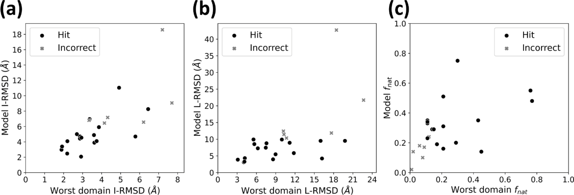
Relationship between domain modeling quality and fitted model quality. Each subplot shows CAPRI statistics for the worst (by I-RMSD) domain from the highest-ranked model (the first hit) of acceptable quality (or from the best I-RMSD model if no models of acceptable quality) vs the same fitted model statistics for each target. (a), I-RMSD. (b), L-RMSD. (c), fnat, the fraction of native contacts.
As seen in Table 2, all targets with at least one domain without a CAPRI-acceptable model failed to produce an acceptable model at the end of the pipeline, with the exception of target PDB 5MGU. In that case, domain models with sufficiently high fnat combined in the flexible fitting to yield a CAPRI-acceptable model with a barely-acceptable L-RMSD of 9.50 Å. While acceptable domain poses were a nearly-necessary condition for final modeling success, they were not a sufficient condition. One target, PDB 3OJW, had 3 combinations of acceptable domain poses available. Indeed, one of the 10,000 fitted models generated was of acceptable quality, with an I-RMSD of 7.4 Å, an L-RMSD of 9.3 Å, and an fnat of 0.18. However, this model was not present in the top 10 models selected by the consensus scoring function. While the interacting regions of a lightly interacting domain model, in this case of the N-terminal domain, may have a low I-RMSD in isolation, the combined interacting regions of both domains do not necessarily superimpose as well. Thus, one particularly misoriented docked domain can spoil the fitted model in terms of the superimposition-based evaluation measures I-RMSD and L-RMSD.
From this result, a broad performance characteristic of Flex-LZerD can be understood. Targets where both domains interact with a single-domain globular receptor via broad interfaces, such as target 1G0Y as shown in Figure 3b, can be considered “easy”, as they are naturally amenable to the rigid-body docking stage on which the flexible fitting depends. On the other hand, targets where at least one domain interacts with confounding sparsity, such as in target 3OJW as previously discussed, can be considered difficult since the flexible fitting cannot fix a misdocked domain. Finally, targets where near-rigid domains cannot be extracted, such as the proteins with intrinsically disordered regions analyzed in the benchmark of IDP-LZerD [42], is out of scope for this protocol. The approach proven in that work for such cases was to divide the ligand protein into many pieces depending on the sequence length and perform rigid-body docking on many fragment models. Thus, such cases are intractable for Flex-LZerD, the current formulation of which only takes two pieces from the ligand.
Figure 3.
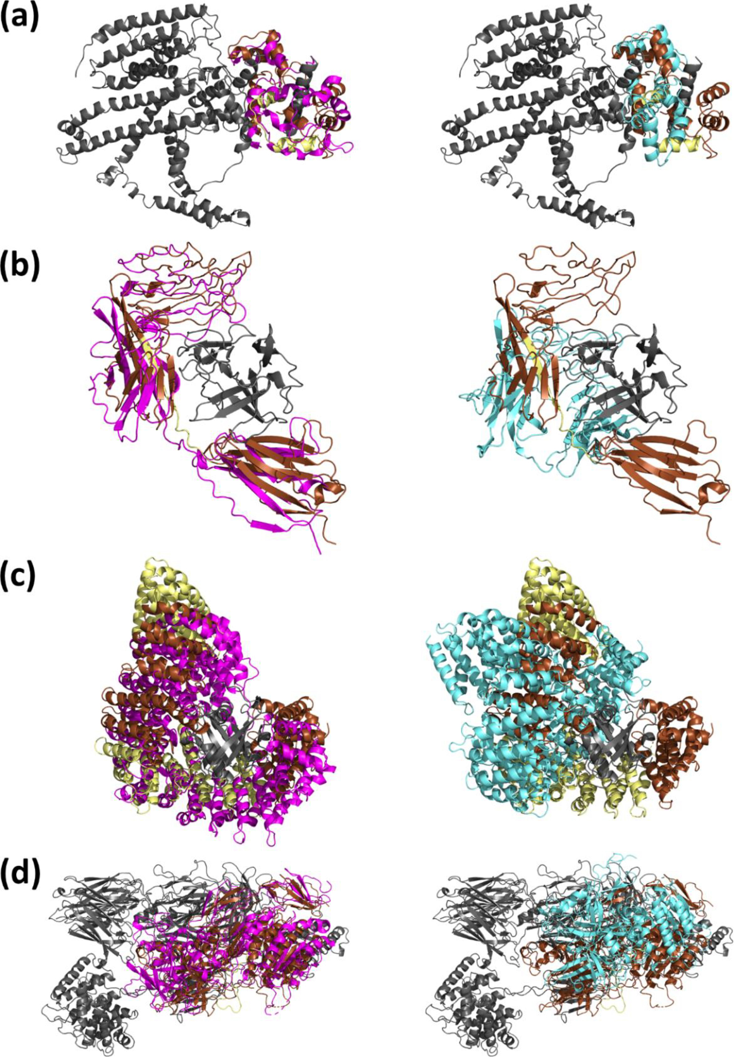
Example modeling of protein-protein complexes. Gray: the receptor structure. Brown: the potions of the native ligand structure corresponding to the extracted domains used for rigid-body domain docking. Yellow: the potions of the native ligand structure which do not correspond to extracted domains. Magenta (left): the lowest I-RMSD Flex-LZerD model output within the top 10. Cyan (right): the lowest I-RMSD model from entirely rigid-body docking. (a) Calmodulin (PDB 5SY1). Flex-LZerD yielded a model with an I-RMSD of 4.5 Å, an L-RMSD of 7.3 Å, and an fnat of 0.33, while rigid-body docking could at best sample a model with an I-RMSD of 11.4 Å, an L-RMSD of 19.3 Å, and an fnat of 0.14. (b) Interleukin-1 receptor type 1 (PDB 1ITB). Flex-LZerD yielded a model with an I-RMSD of 3.9 Å, an L-RMSD of 4.0 Å, and an fnat of 0.29, while rigid-body docking could at best sample a model with an I-RMSD of 14.1 Å, an L-RMSD of 27.9 Å, and an fnat of 0.01. (c) Importin subunit beta-1 (PDB 3EA5). Flex-LZerD yielded a model with an I-RMSD of 2.9 Å, an L-RMSD of 4.3 Å, and an fnat of 0.50, while rigid-body docking could at best sample a model with an I-RMSD of 10.0 Å, an L-RMSD of 17.4 Å, and an fnat of 0.11. (d) Human complement factor B (PDB 2XWB). Flex-LZerD yielded a model with an I-RMSD of 4.9 Å, an L-RMSD of 5.8 Å, and an fnat of 0.35, while rigid-body docking could at best sample a model with an I-RMSD of 19.4 Å, an L-RMSD of 26.9 Å, and an fnat of 0.00.
Protein-nucleic acid targets
Among the protein-nucleic acid targets, we note that all targets produced an acceptable model within the top 10. Even the worst-off two of these targets, 3FDS and 5MGU, were successful yielding CAPRI-acceptable models. Target 3FDS had only a single acceptable pose for each domain to work with, and the final output model had an L-RMSD of 9.4 Å, although it had a high fnat of 0.32. Target 5MGU was similar, with an L-RMSD of 9.5 Å, although it had a high fnat of 0.34, despite technically having no acceptable domain poses to work with. However, two domain poses with sufficiently high fnat combined in the flexible fitting to yield this barely-acceptable full-complex model. This high success rate merits discussion of possible explanations. Proteins which bind nucleic acids tent do interact with the major or minor groove [59], implying a level of molecular shape complementarity regardless of whether the protein is recognizing a specific nucleic acid sequence or nucleic acids more generally. In the initial domain docking pose sampling, LZerD was able to find acceptable positions via its soft surface representation and complementarity-based scoring function. The combined scoring function used for domain and full model scoring in Flex-LZerD also generalized favorably on account of the consensus-based scoring terms used. Unlike in the protein-protein complex case, where many sorts of interfaces and interface geometries exist, docking to a nucleic acid generally requires localization at and orientation to a groove, and shape complementarity is likely lesser in docked models not oriented to a groove. The tendency of the top domain models to be more accurately oriented in the nucleic acid targets than the protein targets can be seen through their typically higher docked-domain fnat scores as shown in Table 2. While this sort of self-selection may be more difficult to take advantage of with less accurate knowledge of the bound structure of the nucleic acid, it demonstrates the ability of Flex-LZerD to take advantage when the nucleic acid of interest is accurately modeled.
Comparison with AlphaFold
In addition to the LZerD protein docking tool, we also considered the potential of AlphaFold-Multimer in this arena. As other protein docking methods specialized for such large conformational changes are not yet developed, this emerging technique may be a future primary alternative. Thus, as part of our evaluation, we used AlphaFold-Multimer [11] to generate models for each target in the benchmark set. Note that the AlphaFold-Multimer models here are not blind predictions. The pretrained models distributed with AlphaFold-Multimer are trained on the entire PDB up to 2018 April 30, and the entirety of the benchmark set was deposited before that date. Thus, the training set of AlphaFold-Multimer included our benchmark set, and the structures in the benchmark set can largely be considered encoded therein. Nonetheless, we consider it a useful forward-looking point of comparison and include it in our analysis (Table 2).
Overall, for the 15 protein-protein targets, AlphaFold-Multimer yielded 9 protein-protein targets with at least CAPRI-acceptable models, for the same number as with Flex-LZerD when the bound receptor was used. Despite the inclusion in its training set of the native structures for all the protein-protein benchmark targets, AlphaFold-Multimer yielded no additional net CAPRI-acceptable hits over Flex-LZerD. However, the hits yielded by AlphaFold-Multimer were usually of overall better quality than the acceptable or better models yielded by Flex-LZerD. In fact, all but 2 of the hits were of at least medium CAPRI quality. In the case where Flex-LZerD modeled a target which AlphaFold-Multimer could not, target PDB 6APX, the receptor was a synthetic monobody. In such a scenario, where there is no coevolutionary interface information to be extracted from multiple sequence alignments, docking-based approaches can still be applied. Here, AlphaFold-Multimer did not even generate any models near the correct interface, and examination of the crystal lattice confirmed that the incorrect models also did not correspond to any crystal packing contacts. The peer-reviewed monomer version of AlphaFold was also tested on our protein-protein benchmark targets by connecting chains with 60-glycine linkers and treating them as a single chain. As shown in Table 2, this treatment yielded far worse modeling accuracy, with CAPRI-acceptable or better hits for only 5 targets. A noticeable limitation of AlphaFold-Multimer were the GPU memory requirements for larger residue counts. Two targets did not run due to this requirement. Furthermore, AlphaFold and AlphaFold-Multimer were completely unable to handle nucleic acids (the bottom half of Table 2).
Modeling examples
Modeling examples of four protein-protein complexes and protein-nucleic acid complexes are provided in Figure 3 and Figure 4, respectively. Among the examples highlighted in Figure 3 is calmodulin, which characteristically wraps around the binding site on its interaction partner [60] to bind via its EF-hand domains and effect a wide variety of downstream functions. Figure 3a shows calmodulin bound to receptor for retinol uptake STRA6 (PDB 5SY1), which requires a large conformational change of 13.8 Å. Using rigid-body docking (right subpanel, cyan), the lowest I-RMSD sampled was 11.4 Å, while Flex-LZerD found a CAPRI-acceptable hit (left subpanel, magenta) with an I-RMSD of 4.5 Å. Rigid body docking could localize calmodulin at the binding site but was naturally incapable of properly orienting both EF-hands and wrapping the binding site. On the other hand, Flex-LZerD did exactly that, generating the kink necessary to bend calmodulin in half and wrap around the binding site on STRA6. Shown next in Figure 3b is interleukin-1 receptor type 1 (IL-1R) bound to interleukin-1 beta (IL-1 beta) (PDB 1ITB) [61], which requires a conformational change of 18.2 Å. In this target, IL-1R is initially closed relative to the bound structure. In fact, the binding site is totally inaccessible, with rigid-body docking unable to attain an I-RMSD better than 14.1 Å (right subpanel, cyan). Here, Flex-LZerD was able to open up IL-1R to admit IL-1 beta, yielding a CAPRI-acceptable hit with an I-RMSD of 3.9 Å (left subpanel, magenta). The progression of fitting IL-1R is illustrated in Figure 1b and Supplemental Video S1. In the beginning, IL-1R is merely centered on the docked domains. IL-1R then quickly opens up in the early iterations. Next, the C-terminal end of the ligand rotates, reorienting following the docked C-terminal domain. As IL-1b enters the equation, the steric complementarity at the interface emerges. Finally, the model described above results as the fitting finishes. This example demonstrated that flexible fitting could start from a closed conformation model of a protein, could open the model in a way that accepts the protein’s binding partner, and could produce a model close to the native structure. Figure 3c shows importin subunit beta-1 binding to GTP-binding nuclear protein Ran (PDB 3EA5), a key stage in the nuclear import cycle [48], which requires a conformational change of 10.1 Å. From the unbound state of importin, rigid body docking was unable to attain an I-RMSD better than 10.0 Å (right subpanel, cyan). Though the binding site is not outright blocked, the solenoid in its unbound state is still closed relative to the bound. Flex-LZerD was able to open importin to accommodate Ran, yielding a CAPRI-acceptable hit with an I-RMSD of 2.9 Å (left subpanel, magenta). The progression of fitting importin is illustrated in Supplemental Video S2. In the beginning, importin is merely centered on the docked HEAT domains. Then, importin’s twisted shape quickly opens up, creating enough steric void to admit Ran. As the structure of Ran is included in the fitting, we quickly obtain our final structure. this example demonstrated that even when the domains used are not globular, flexible fitting could start from a closed conformation model of a protein, could open the model in a way that accepts the protein’s binding partner, and could produce a model close to the native structure. Finally, Figure 4d shows human complement factor B (CFB) binding complement C3 (PDB 2XWB), a core part of amplification in the complement system [26] which requires a conformational change of 20.2 Å. Here the binding site is not blocked, but still must take on a different conformation to actually form an interface. Rigid-body docking was only able to reach an I-RMSD of 19.4 Å (right subpanel, cyan), but Flex-LZerD was able to fit the interface and generate a CAPRI-acceptable hit with an I-RMSD of 5.0 Å (left subpanel, magenta).
Figure 4.
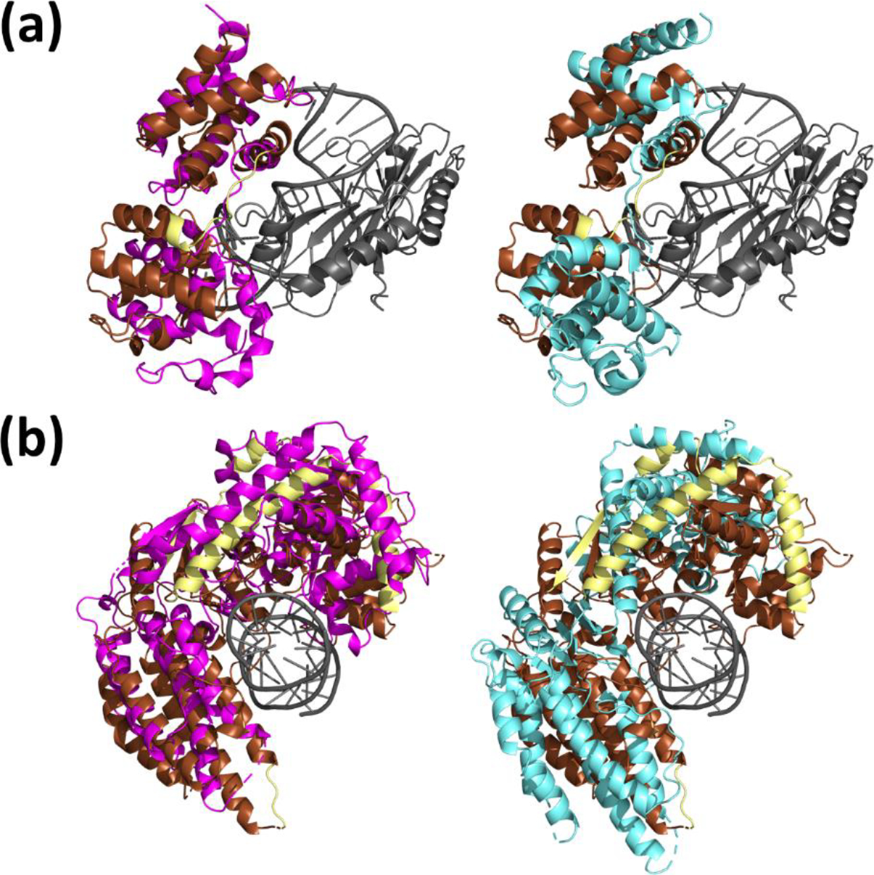
Example modeling of protein-nucleic acid complexes. Gray: the receptor structure. Brown: the potions of the native ligand structure corresponding to the extracted domains used for rigid-body domain docking. Yellow: the potions of the native ligand structure which do not correspond to extracted domains. Magenta (left): the lowest I-RMSD Flex-LZerD model output within the top 10. Cyan (right): the lowest I-RMSD model from entirely rigid-body docking. (a) Transcription initiation factor IIB (PDB 1C9B). Flex-LZerD yielded a model with an I-RMSD of 4.1 Å, an L-RMSD of 9.9 Å, and an fnat of 0.23, while rigid-body docking could at best sample a model with an I-RMSD of 8.7 Å, an L-RMSD of 16.5 Å, and an fnat of 0.03. (b) Antiviral innate immune response receptor RIG-I (PDB 7JL1). Flex-LZerD yielded a model with an I-RMSD of 4.7 Å, an L-RMSD of 5.5 Å, and an fnat of 0.19, while rigid-body docking could at best sample a model with an I-RMSD of 11.2 Å, an L-RMSD of 7.4 Å, and an fnat of 0.02.
Flex-LZerD was also able to model a variety of conformational changes in nucleic acid-binding targets (Figure 4). Nucleic acids are not generally handled by current state-of-the-art deep learning methods for macromolecular structure prediction. Highlighted fin Figure 4a is transcription initiation factor IIB (TFIIB), essential for transcription initiation [62] bound to DNA. TFIIB must form interactions with both the major and minor groove of the DNA to bind. For the blind ligand input, we used a structure of transcription initiation factor IIB that was solved in isolation (PDB 5WH1). Domains were cut from the unbound structure by separating its two cyclin-like domains, removing their flexible linker [63] from Ala201 to Asp210. This binding consequently requires an overall conformational change of 12.2 Å. The rigid-body docking was only able to reach 8.7 Å I-RMSD (right subpanel, cyan). Flex-LZerD on the other hand was able to conform TFIIB to both the major and minor grooves with an I-RMSD of 4.1 Å (left subpanel, magenta) using N-terminal and C-terminal domain poses modeled to 2.5 Å I-RMSD and 2.6 Å I-RMSD, respectively. The progression from the input unbound TFIIB structure to this fitted model is illustrated in Supplemental Video S3. Due to the simple TFIIB structure and the absence of bulky receptor structure taking up volume around the interface, this fitting was particularly smooth. Both domains quickly reorient to match their separately docked counterparts. Steric complementarity with the receptor is quickly achieved as well. This example demonstrated that even when the receptor is not a protein, flexible fitting could start from a closed conformation model of a protein, could close the model in a way that accepts the protein’s binding partner, and could produce a model close to the native structure. Other protein-nucleic acid interactions can feature flexible interfaces encompassing more of the nucleic acid. Figure 4b shows the antiviral innate immune response receptor RIG-I (RIG-I), part of the innate immune system in vertebrates [64],bound to dsRNA through a conformational change of 13.2 Å. To properly bind the dsRNA, RIG-I must close around the double helix. Rigid body docking was able to sample a conformation with 11.2 Å I-RMSD (right subpanel, cyan), which places RIG-I at the correct location, but fails to form most of the interface. Flex-LZerD on the other hand yielded a model with an I-RMSD of 4.7 Å, which successfully wrapped around the dsRNA.
Computational requirements
Flex-LZerD was tested on a cluster of compute nodes (“Bell” at Purdue University) each with two AMD EPYC 7662 64-core CPUs and 256GB of RAM. The running time of the pipeline increases with the length of the input flexible ligand protein, in particular the time required for the normal mode calculations and the energy minimization. At the low end, the running time is dominated by the energy minimization. However, the normal mode calculations have a higher growth order and begin to surpass the energy minimization in running time roughly in the regime of greater than 500 residues (Figure 5). To manage the resources required, we limited the fitting with each individual domain pair to 4 hours each, the time limit for the readily available standby scheduling on the Bell cluster. Under typical cluster usage conditions where we could use about 10–20 nodes, a single target would finish all 10,000 fitting runs in 1 to 2 days. The fastest ligand in the benchmark was PDB 1GV2 with 159 residues, which took 10,037 CPU core-hours (took us about 1 day on the cluster). On the other hand, the slowest ligand was PDB 3ND2, which exceeded the 4-hour time limit. Sufficient timing data was generated, however, to calculate that running 3ND2 for all 500 iterations would have taken a total of 157,490 CPU core-hours (which took us about 2 days with the time limit on the cluster). The computational time could be shortened with tricks such as increasing the RTB block size to span multiple residues, although this would require careful tuning.
Figure 5.
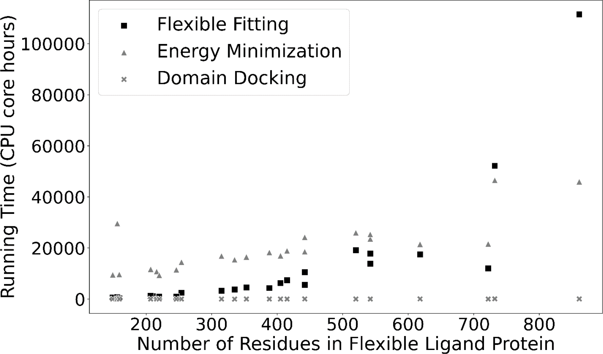
The size of the flexible ligand protein vs the running time of Flex-LZerD across all targets, broken down by pipeline stage. Flexible Fitting, Energy Minimization, and Domain Docking indicate the total running time for a target spent on normal mode calculation and deformation, Phenix energy minimization, and domain docking using LZerD, respectively. Running times were linearly extrapolated to the full 500 iterations where necessary. Since component running times were stable across all iterations, simple linear extrapolation was suitable.
Discussions
In this work, we have shown that flexible fitting is capable of modeling large scale conformational changes in complex assembly, including in protein-nucleic acid docking that is not handled by state-of-the-art deep learning methods. The highly generalizable nature of this form of modeling is expected to enable its application to other modeling categories not covered by this work, especially in integrative contexts.
This work provides a method for specific docking cases where the ligand protein has structured domains that can dock as rigid fashion and expected to have a large conformational change upon docking, which was not properly addressed before. In realistic application of protein docking, different types of docking methods developed by the community would need to be combined in a pipeline. In the most generic case with no information beyond initial subunit structures, regular docking methods with as LZerD [12] or HADDOCK can be used to model a complex. However, the more information is known about the protein complex, the more comprehensive the modeling can be. If distance restraints between interacting or non-interacting residue pairs are known from experiments such as nuclear magnetic resonance (NMR) or electron paramagnetic resonance (EPR), they can be applied in methods such as the LZerD webserver [14, 15], ClusPro [5], and HADDOCK [65]. When symmetry information is known, tools such as the LZerD webserver, M-ZDOCK [66], and SAM [67, 68] can take advantage. IDP-LZerD [42] can be used when one subunit is known to be intrinsically disordered, while for shorter peptide chains, MDockPeP [69] can be used. For higher-order heteromers, multiple docking method such as Multi-LZerD [70] or RL-MLZerD [71] can be used, which can even predict assembly order [72]. Finally, in cases where enough information is available to determine domains of flexible proteins, methods such as Flex-LZerD, presented here, can be applied. Ligand conformational change can feasibly be ascertained by spectroscopic, fluorescence, or other biophysical techniques. In the event of uncertain information, multiple tools can be run simultaneously as part of the modeling workflow. However, they are generally developed and employed independently from each other.
Protein docking is also indispensable step in modeling atomic structures from cryo-electron microscopy density maps [73, 74], where expert microscopists and many modern automated methods consider the modeling of domains and fragments to highly-resolved regions [75, 76]. The flexible fitting in this work can be readily fed such fragments, as in principle the size of domains input does not matter. Methods for modeling intrinsically disordered proteins also often work with individually modeled fragments [42]. Thus, we anticipate future development along these directions.
MATERIALS AND METHODS
Dataset construction
Two datasets were constructed for this work. The testing benchmark set was constructed by running a BLAST [77] query of all sequences found in complexes in PDB against all sequences found in PDB to find unbound structures. Then, hits with at least 90% sequence identity and at least 10.0 Å RMSD of conformational difference were retained. This cutoff was relaxed to 7.0 Å for nucleic acid targets. Benchmark examples were then selected by expert manual inspection, selecting for examples where the 10.0 Å conformational difference was due to large scale changes in the ligand protein and not, for example, due to differently packed tails or domain swapping. Duplicate hits were filtered out. The final benchmark set of 23 targets is detailed in Table 1. It includes 15 protein-protein complexes and 8 protein-DNA complexes. Among the 15 protein-protein docking cases, 9 of them have unbound receptor structure. The training set was taken from the benchmark set of a ClustENM-HADDOCK work [20, 35] which examined docking at lower scales of conformational change. Two examples, PDB 1IRA and PDB 1IBR, were excluded from the training set because they were already present in the benchmark set. The 9 training set targets are detailed in Supplemental Table S2.
Table 1.
The benchmark set used to evaluate Flex-LZerD. N/a indicates that an unbound structure was not available in PDB.
| Ligand protein name | Native complex PDB | Total complex #residues | Unbound receptor PDB | Unbound ligand PDB | Ligand conformational difference (RMSD) Cα/full | Ligand #residues | Receptor #residues | Nondomain #residues |
|---|---|---|---|---|---|---|---|---|
|
| ||||||||
| Calmodulin | 5SY1 (A:C) | 819 | n/a | 1CLL (A) | 13.8/14.1 | 149 | 670 | 28 |
| Interleukin-1 receptor type 1 | 1ITB (A:B) | 468 | 1HIB | 1G0Y (R) | 18.2/18.4 | 315 | 153 | 14 |
| Importin subunit beta-1 | 3EA5 (A:B) | 1077 | 2MMC | 3ND2 (A) | 10.1/10.2 | 861 | 216 | 465 |
| Transcription inhibitor protein Gfh1 | 3AOI (ABCDEPQ:X) | 3540 | n/a | 2F23 (A) | 13.4/13.5 | 156 | 3384 | 10 |
| Dual specificity protein phosphatase 1 | 6APX (B:A) | 616 | n/a | 6D66 (A) | 11.6/11.9 | 520 | 96 | 45 |
| Immunoglobulin lambda variable 2–8 | 1DCL (B:A) | 432 | 6P95 | 2MCG (1) | 12.9/13.0 | 216 | 216 | 11 |
| Ribosomal protein L11 methyltransferase | 2NXN (B:A) | 401 | 2E36 | 1UFK (A) | 11.0/11.2 | 254 | 147 | 10 |
| Protein SdcA | 6CP2 (B:A) | 696 | 1C4Z | 4TRG (A) | 10.6/10.8 | 542 | 154 | 30 |
| Protein SdcA | 6CP2 (C:A) | 620 | 3OJ3 | 4TRG (A) | 10.6/10.8 | 542 | 78 | 30 |
| NADPH-cytochrome P450 reductase | 3WKT (C:A) | 885 | 1DVE | 3OJW (A) | 11.5/11.7 | 618 | 267 | 15 |
| Fibroblast growth factor receptor 2 | 1EV2 (A:E) | 352 | 1BAS | 1E0O (E) | 12.0/11.9 | 220 | 132 | 13 |
| HIV p51 subunit | 6BSJ (ADR:B) | 1044 | n/a | 4KSE (B) | 13.5/13.3 | 442 | 602 | 29 |
| Human complement factor B | 2XWB (AB:F) | 2286 | 2A74 | 2OK5 (A) | 20.2/20.3 | 732 | 1554 | 21 |
| Carbon monoxide dehydrogenase corrinoid/iron-sulfur protein, gamma subunit | 4C1N (DJ:C) | 1260 | n/a | 2YCL (A) | 13.9/14.0 | 442 | 818 | 15 |
| Cullin-5/E3 ubiquitin-protein ligase RBX1 | 4F52 (AB:E) | 984 | n/a | 3DQV (CR) | 20.7/20.4 | 388 | 596 | 9 |
|
Nucleic acid-binding targets
|
||||||||
| Transcription initiation factor IIB | 1C9B (BCD:A) | 421 | n/a | 5WH1 (A) | 12.2/12.4 | 207 | 214 | 10 |
| Transcriptional activator Myb | 1H89 (ABDE:C) | 337 | n/a | 1GV2 (A) | 7.1/7.5 | 159 | 178 | 7 |
| RP-A 70 kDa DNA-binding subunit | 1JMC (B:A) | 256 | n/a | 1FGU (A) | 8.3/8.5 | 246 | 8 | 22 |
| Elongation factor TU | 1TTT (D:A) | 482 | n/a | 1AIP (A) | 11.4/11.5 | 405 | 77 | 12 |
| DNA polymerase IV | 2IMW (ST:P) | 379 | n/a | 3FDS (A) | 16.3/17.0 | 353 | 26 | 25 |
| DNA polymerase beta | 6NKZ (DPT:A) | 366 | n/a | 1BPD (A) | 11.9/11.9 | 335 | 31 | 18 |
| Antiviral innate immune response receptor RIG-I | 7JL1 (XY:A) | 750 | n/a | 4ON9 (A) | 13.2/13.3 | 722 | 28 | 22 |
| Phenylalanine-tRNA ligase, mitochondrial | 3TUP (T:A) | 491 | n/a | 5MGU (A) | 18.7/18.9 | 415 | 76 | 24 |
Rigid-body docking of domains
Each ligand protein structure domain was docked with the receptor structure using LZerD [12, 49]. LZerD is a shape complementarity-based rigid-body docking which uses a soft representation of the molecular surface to achieve tolerance to some small conformational change. Using geometric hashing, LZerD rapidly generates many docking poses, which are then scored according to their surface shape complementarity. For each target complex, domain models were manually generated for the ligand by identifying rigid regions and removing the intervening residues. For each input domain, the set of docked models generated by LZerD was ordered by the LZerD shape score and truncated to a set of 50,000 models. Then, each set was clustered with an RMSD cutoff of 4.0 Å.
Domain scoring
For selecting docked domain poses, we constructed a combined scoring function generalized from methods used in the scoring of IDP-LZerD[42]. This scoring function uses logistic regression to combine the knowledge-based scoring functions GOAP [78], DFIRE [79], and ITScorePro [80], which are the three scoring functions combined in the usual ranksum score for docking [13, 50, 51], as well as LZerD shape complementarity score, the number of docking decoys in the cluster from 4 Å RMSD clustering, binding site consensus terms (BSCR,5, BSCL,5. BSCRL,5. BSCR,10, BSCL,10, BSCRL,10) representing residue interaction agreement within the docking pool, and order statistic terms (OS(1), OS(2), and OS(3)) highlighting extreme values among the other scoring terms for each model.
The LZerD shape complementarity scores and the cluster sizes are taken from the previous initial docking stage. The binding site consensus terms BSCx,y quantify the frequency of residue-residue interactions observed in docking models generated in the domain docking. There are six binding site consensus terms in total, calculated from the combinations of two interaction distance cutoffs (5.0 Å and 10.0 Å) and three sets of interface residues considered (receptor, ligand, and both). 5.0 Å and 10.0 Å were used as cutoffs following the definitions of protein-protein interactions in the CAPRI evaluation criteria. For example, BSCR,5 considers interface residues in the Receptor using a 5.0 Å distance cutoff. More specifically, they are defined as follows: given a docked model pool P (here typically 10,000 to 50,000 docking decoys) and an interaction distance cutoff Rmax (here 5.0 Å and 10.0 Å) we define a to be the residues in model m which interact with x, in other words the set of residues in model m in a the opponent molecule from residue x that are within distance Rmax of x. For example, if x is from the receptor, residues are counted from the interacting protein domain. Then, each residue x in the in all subunits (both receptor and ligand) is assigned an occupancy score Occ[x] indicating the frequency with which that residue appears as part of a residue-residue contact pair across the interface in the model pool P, calculated by simply counting the encountered interactions:
| (1) |
where # counts the number of binding residues (B) with x within the Rmax distance. Then, to calculate the binding site consensus score for a docking model, the interface residues being considered in the model are counted, weighted by the occupancy that was just calculated. Formally, denoting as Q the receptor side, the ligand side, or both sides of the interface as determined by Rmax, each model m ∈ P is assigned the binding site consensus score :
| (2) |
The order statics terms are to consider if any score prefers a model with a high significance or not even if it is not the consensus among all the scoring terms To prepare, first, each score was normalized to a Z-score. A Z-score of a raw score is defined as: (Raw_score – Average)/Standard_Deviation. The average and the standard deviation are computed from the score distribution of decoys of the target. Scoring terms where more positive values should be more favorable, i.e. LZerD shape complementarity scores, cluster sizes, and binding site consensus scores, were each multiplied by −1 so that lower is more favorable for all component scores. Thus, for all the scoring terms a negative large Z-score is favorable. From these, order statistic terms were calculated for the Z-scores of the scoring terms. To compute the order statistics of OS(1) of a model, we first check the Z-sores of all the scoring terms for the model, and select the smallest (the most significant) Z-score. In the same way, OS(2) and OS(3) are the second and the third smallest Z-scores among all the Z-scores of all the scoring terms. A first-order term of this form, OS(1), was previously used successfully in IDP-LZerD [42], and here we expanded it to include OS(2) and OS(3). For example, if a model has Z-scores of −1.6, −2.3, and −0.4 for the cluster size, BSCR,5, and ITScorePro, respectively, and some arbitrary positive-valued Z-scores (i.e. insiginificant scores) for the nine other scoring terms, then OS(1), OS(2), and OS(3) that model will be −2.3, −1.6, and −0.4, respectively. In this work, we generalized up to the third order by including OS(1), OS(2), and OS(3) in the combined scoring function.
The component scores GOAP, DFIRE, ITScorePro, ranksum, the LZerD shape score, LZerD cluster size, BSCR,5, BSCL,5. BSCRL,5. BSCR,10, BSCL,10, BSCRL,10, OS(1) OS(2), and OS(3), were then finally combined in a logistic regression model. To optimize the logistic regression weights, docked models were generated for each target in the training dataset using the same procedure as above. CAPRI statistics were then calculated for each model. Each model was labeled positive if it was of acceptable CAPRI quality, and negative if it was not. Each model was then weighted to balance the number of positive and negative cases within each target. Then, the logistic regression model was trained using all the models for all the training targets. The resulting scoring function was used to rescore the docked domain models after the clustering stage. The training set performance is shown in Supplemental Table S3.
Anisotropic network model
In Flex-LZerD, we use an elastic network model to deform the ligand structure into agreement with the docked domains, in particular the anisotropic network model (ANM) [81–83]. In an ANM, atoms are considered as point masses with a simple harmonic potential constructed by considering initial distances between atoms. The general idea is that principal components of possible large-scale motions can be extracted by coupling the system in this way. Here, atoms are connected if they are within 15.0 Å of each other. Thus, for each pair of atoms i and j among the total n atoms, we build up a potential U as follows:
| (3) |
with the overall potential computed as the sum of the pairs:
| (4) |
where γ is a Hookean spring constant, which is set to 1, sij is the distance between two atoms, and is the initial distance between two atoms.
To generalize the 1D single-spring case with potential and restoring force F = −γΔs, we generalize the stiffness to the Hessian H of the potential and the 1D displacement Δs to the 3D multi-point displacement :
| (5) |
where H is 3n × 3n. We are not interested in particular values of force. Instead, we want to extract the normal modes of this system, the directions and relative displacements that will set the masses oscillating in simple harmonic motion in phase with each other. This requires that each atom be moving along a particular line with forces and displacements parallel. Thus, we can formulate the normal mode extraction as an eigendecomposition problem:
| (6) |
The eigendecomposition will give us 3n − 6 normal modes vi (6 eigenvectors are lost as degenerate to the bulk translational and rotational degrees of freedom) each with a corresponding frequency . By convention, the normal modes are arranged in order of nondecreasing frequency. Following common practice, the 20 slowest modes were taken for use in the iterative flexible fitting.
Rotations and translations of blocks
Instead of using the basic ANM, we used the rotations and translations of blocks (RTB) [55] method, which is capable of treating individual amino acids rigid bodies, which preserves the low-frequency behavior and is less computationally expensive. Instead of the above full formulation (Eqs. 3–6), which requires an expensive computation of 3n × 3n Hessian matrix, RTB linearizes SE(3) transformations of N blocks (residues). Based on the mass of each block and atom and inertia tensor of each block, projection matrices are constructed to convert the blocks into rigid bodies engaged in infinitesimal translations and rotations:
| (7) |
| (8) |
Where k identifies a particular atom, b identifies a particular block, 3 × 3 matrices and correspond to translation and rotation projections for atom k, mk and qk are the mass and coordinates of atom k, Mb and are the mass and center-of-mass coordinates of block b. Stacking these atom-wise projections into block-wise projections row-wise yields 3Nb × 3 matrices and , where Nb is the number of atoms in b. These block projections are assembled into a 3n × 6N block-diagonal matrix as follows:
| (9) |
This whole-structure projection matrix is then used to project the mass-weighted Hessian into the RTB subspace. Thus, the 3n × 3n original Hessian is reduced to a merely 6N × 6N substitute. It is subsequently diagonalized to extract normal modes within the subspace:
| #(10) |
This enables a faster diagonalization while preserving the large-scale properties of the whole elastic network. To recover these modes in the form of all-atom displacements, we simply take . In this work, calculation of and projection to RTB normal modes using partial structures was implemented using the ProDy framework [84].
Iterative fitting to docked domains
As previously stated, normal modes only allow displacement in straight lines. Even adding multiple normal modes simultaneously, normal modes alone here do not allow curvilinear motion. Extremely large conformational changes, however, require curvilinear motion. To accomplish curvilinear motion, modes are restricted to small amplitude motion. Then, after such a small displacement, the Hessian is recalculated and re-diagonalized. Thus, using many line segments, curvilinear motion is accomplished. This iterative pipeline is illustrated in Figure 1. In the context of Flex-LZerD, mode amplitudes are selected to follow the displacements that would bring atom positions in the unbound ligand structure to coincide with the docked domains. The twist of course is that no such displacements are defined for the atoms which are present in the unbound structure but not in the docked domains. To impute displacements for the regions not modeled by domains, the normal modes are masked to exclude unmodeled atoms prior to projecting the displacements thereon. Once amplitudes have been obtained for the modes in this way, the amplitudes are attenuated by a factor of 0.05 and applied to the unmasked modes. An attenuation of 0.05 was chosen to produce few violations over 0.1 Å of the typical Cα-Cα distance of 3.8 Å. Thus, guided by the information from partial complex assembly by domains, the entire assembly can be modeled.
Minimization of geometric restraints
Minimization of molecular geometry violations, such as from bond lengths, van der Waals interactions, and torsion angles, during each iteration was accomplished within the PHENIX [85] software framework using an L-BFGS minimizer within the “mmtbx.refinement.geometry_minimization” library. This minimization was always applied to the ligand structure. Additionally, every 10th iteration after the 100th, the receptor structure was also included in the minimization. The periodic inclusion of the receptor is meant to help the ligand conform to the receptor surface, while the 100-iteration delay is meant to accommodate any steric overlap in the initial positioning of the ligand.
Fitted model scoring
Fitted models are scored using the same scoring function as in the docked domain scoring stage. Here, instead of the binding site consensus terms being freshly calculated, the values from the docked domain scoring stage are used.
LZerD rigid-body docking
For comparison with the flexible docking, each target was docked without considering flexibility using LZerD [12, 49], which can be downloaded from https://kiharalab.org/proteindocking/lzerd.php. LZerD, just as in the rigid-body docking of domains described above, is a shape complementarity-based rigid-body docking which uses a soft representation of the molecular surface to achieve tolerance to some small conformational change. Using geometric hashing, LZerD rapidly generates many docking poses, which are then scored according to their surface shape complementarity. For each target, the set of docked models generated by LZerD was ordered by the LZerD shape score and truncated to a set of 50,000 models. Then, each set was clustered with an RMSD cutoff of 4.0 Å. Ordinarily, LZerD models are scored by ranksum[13, 14, 51]. However, to highlight the inaccessibility of the benchmark set to rigid-body docking, we instead simply selected the model with the lowest I-RMSD (i.e. the best model among generated docking poses). The results of these rigid-body docking runs, which had a 100% failure rate as expected, are shown in Table 2.
AlphaFold and AlphaFold-Multimer
AlphaFold [10] and AlphaFold-Multimer [11] models were generated using version 2.0.1 (https://github.com/deepmind/alphafold/releases/tag/v2.0.1) and version 2.2.2 (https://github.com/deepmind/alphafold/releases/tag/v2.2.2), respectively, of DeepMind’s released AlphaFold software package. For all required databases, the default versions linked to by AlphaFold’s install script were used. For all applicable targets, AlphaFold was run without the use of templates. When using the original monomeric version of AlphaFold, the ligand sequence was concatenated to the receptor sequence with a 60-glycine linker. Other configurable parameters were left at their default values. For each applicable target, 5 models were thus generated and ranked according to AlphaFold-Multimer’s output score. CAPRI statistics were then calculated to evaluate model accuracy, and the accuracy of the first CAPRI-acceptable model was reported (see Table 2).
Supplementary Material
ACKNOWLEDGEMENTS
The authors are grateful to Information Technology at Purdue, West Lafayette, Indiana for providing computational resources.
FUNDING
This work was partly supported by the National Institutes of Health (R01GM123055, R01GM133840), the National Science Foundation (DBI2003635, DBI2146026, CMMI1825941, and MCB1925643) and the Purdue Institute of Drug Discovery. CC was supported by NIGMS-funded predoctoral fellowship to CC (T32 GM132024). The contents of this work are solely the responsibility of the authors and do not necessarily represent the official views of the funding agencies.
Footnotes
DECLARATIONS OF INTEREST
The authors declare no conflict of interest.
REFERENCES
- 1.Berman HM, Battistuz T, Bhat TN, Bluhm WF, Bourne PE, Burkhardt K, et al. (2002). The Protein Data Bank. Acta Crystallogr D Biol Crystallogr. 58, 899–907. [DOI] [PubMed] [Google Scholar]
- 2.Aderinwale T, Christoffer CW, Sarkar D, Alnabati E, Kihara D (2020). Computational structure modeling for diverse categories of macromolecular interactions. Curr Opin Struct Biol. 64, 1–8. [DOI] [PMC free article] [PubMed] [Google Scholar]
- 3.Mintseris J, Pierce B, Wiehe K, Anderson R, Chen R, Weng Z (2007). Integrating statistical pair potentials into protein complex prediction. Proteins. 69, 511–20. [DOI] [PubMed] [Google Scholar]
- 4.Dominguez C, Boelens R, Bonvin AM (2003). HADDOCK: a protein-protein docking approach based on biochemical or biophysical information. J Am Chem Soc. 125, 1731–7. [DOI] [PubMed] [Google Scholar]
- 5.Kozakov D, Hall DR, Xia B, Porter KA, Padhorny D, Yueh C, et al. (2017). The ClusPro web server for protein-protein docking. Nat Protoc. 12, 255–78. [DOI] [PMC free article] [PubMed] [Google Scholar]
- 6.Lyskov S, Gray JJ (2008). The RosettaDock server for local protein-protein docking. Nucleic Acids Res. 36, W233–8. [DOI] [PMC free article] [PubMed] [Google Scholar]
- 7.Ritchie DW, Venkatraman V (2010). Ultra-fast FFT protein docking on graphics processors. Bioinformatics. 26, 2398–405. [DOI] [PubMed] [Google Scholar]
- 8.Torchala M, Moal IH, Chaleil RA, Fernandez-Recio J, Bates PA (2013). SwarmDock: a server for flexible protein-protein docking. Bioinformatics. 29, 807–9. [DOI] [PubMed] [Google Scholar]
- 9.de Vries S, Zacharias M (2013). Flexible docking and refinement with a coarse-grained protein model using ATTRACT. Proteins. 81, 2167–74. [DOI] [PubMed] [Google Scholar]
- 10.Jumper J, Evans R, Pritzel A, Green T, Figurnov M, Ronneberger O, et al. (2021). Highly accurate protein structure prediction with AlphaFold. Nature. [DOI] [PMC free article] [PubMed] [Google Scholar]
- 11.Evans R, O’Neill M, Pritzel A, Antropova N, Senior A, Green T, et al. (2021). Protein complex prediction with AlphaFold-Multimer. bioRxiv. 2021.10.04.463034. [Google Scholar]
- 12.Venkatraman V, Yang YD, Sael L, Kihara D (2009). Protein-protein docking using region-based 3D Zernike descriptors. BMC Bioinformatics. 10, 407. [DOI] [PMC free article] [PubMed] [Google Scholar]
- 13.Christoffer C, Terashi G, Shin WH, Aderinwale T, Maddhuri Venkata Subramaniya SR, Peterson L, et al. (2020). Performance and enhancement of the LZerD protein assembly pipeline in CAPRI 38–46. Proteins. 88, 948–61. [DOI] [PMC free article] [PubMed] [Google Scholar]
- 14.Christoffer C, Chen S, Bharadwaj V, Aderinwale T, Kumar V, Hormati M, et al. (2021). LZerD webserver for pairwise and multiple protein-protein docking. Nucleic Acids Res. [DOI] [PMC free article] [PubMed] [Google Scholar]
- 15.Christoffer C, Bharadwaj V, Luu R, Kihara D (2021). LZerD Protein-Protein Docking Webserver Enhanced With de novo Structure Prediction. Front Mol Biosci. 8, 724947. [DOI] [PMC free article] [PubMed] [Google Scholar]
- 16.Lensink MF, Nadzirin N, Velankar S, Wodak SJ (2020). Modeling protein-protein, protein-peptide, and protein-oligosaccharide complexes: CAPRI 7th edition. Proteins. 88, 916–38. [DOI] [PubMed] [Google Scholar]
- 17.Lensink MF, Brysbaert G, Nadzirin N, Velankar S, Chaleil RAG, Gerguri T, et al. (2019). Blind prediction of homo- and hetero-protein complexes: The CASP13-CAPRI experiment. Proteins. 87, 1200–21. [DOI] [PMC free article] [PubMed] [Google Scholar]
- 18.Kuroda D, Gray JJ (2016). Pushing the Backbone in Protein-Protein Docking. Structure. 24, 1821–9. [DOI] [PMC free article] [PubMed] [Google Scholar]
- 19.Harmalkar A, Gray JJ (2021). Advances to tackle backbone flexibility in protein docking. Curr Opin Struct Biol. 67, 178–86. [DOI] [PMC free article] [PubMed] [Google Scholar]
- 20.Kurkcuoglu Z, Bonvin A (2020). Pre- and post-docking sampling of conformational changes using ClustENM and HADDOCK for protein-protein and protein-DNA systems. Proteins. 88, 292–306. [DOI] [PMC free article] [PubMed] [Google Scholar]
- 21.Palamini M, Canciani A, Forneris F (2016). Identifying and Visualizing Macromolecular Flexibility in Structural Biology. Front Mol Biosci. 3, 47. [DOI] [PMC free article] [PubMed] [Google Scholar]
- 22.Qin BY, Bewley MC, Creamer LK, Baker HM, Baker EN, Jameson GB (1998). Structural basis of the Tanford transition of bovine beta-lactoglobulin. Biochemistry. 37, 14014–23. [DOI] [PubMed] [Google Scholar]
- 23.Bennett WS, Huber R (1984). Structural and functional aspects of domain motions in proteins. CRC Crit Rev Biochem. 15, 291–384. [DOI] [PubMed] [Google Scholar]
- 24.Korostelev A, Noller HF (2007). Analysis of structural dynamics in the ribosome by TLS crystallographic refinement. J Mol Biol. 373, 1058–70. [DOI] [PMC free article] [PubMed] [Google Scholar]
- 25.Williams BB, Van Benschoten AH, Cimermancic P, Donia MS, Zimmermann M, Taketani M, et al. (2014). Discovery and characterization of gut microbiota decarboxylases that can produce the neurotransmitter tryptamine. Cell Host Microbe. 16, 495–503. [DOI] [PMC free article] [PubMed] [Google Scholar]
- 26.Forneris F, Ricklin D, Wu J, Tzekou A, Wallace RS, Lambris JD, et al. (2010). Structures of C3b in complex with factors B and D give insight into complement convertase formation. Science. 330, 1816–20. [DOI] [PMC free article] [PubMed] [Google Scholar]
- 27.Menting JG, Whittaker J, Margetts MB, Whittaker LJ, Kong GK, Smith BJ, et al. (2013). How insulin engages its primary binding site on the insulin receptor. Nature. 493, 241–5. [DOI] [PMC free article] [PubMed] [Google Scholar]
- 28.Tidow H, Nissen P (2013). Structural diversity of calmodulin binding to its target sites. FEBS J. 280, 5551–65. [DOI] [PubMed] [Google Scholar]
- 29.Stewart M (2007). Molecular mechanism of the nuclear protein import cycle. Nat Rev Mol Cell Biol. 8, 195–208. [DOI] [PubMed] [Google Scholar]
- 30.Peterson L, Jamroz M, Kolinski A, Kihara D (2017). Predicting Real-Valued Protein Residue Fluctuation Using FlexPred. Methods Mol Biol. 1484, 175–86. [DOI] [PubMed] [Google Scholar]
- 31.Jamroz M, Kolinski A, Kihara D (2012). Structural features that predict real-value fluctuations of globular proteins. Proteins. 80, 1425–35. [DOI] [PMC free article] [PubMed] [Google Scholar]
- 32.Li H, Chang YY, Yang LW, Bahar I (2016). iGNM 2.0: the Gaussian network model database for biomolecular structural dynamics. Nucleic Acids Res. 44, D415–22. [DOI] [PMC free article] [PubMed] [Google Scholar]
- 33.Zhang Y, Zhang S, Xing J, Bahar I (2021). Normal mode analysis of membrane protein dynamics using the vibrational subsystem analysis. J Chem Phys. 154, 195102. [DOI] [PMC free article] [PubMed] [Google Scholar]
- 34.Oliwa T, Shen Y (2015). cNMA: a framework of encounter complex-based normal mode analysis to model conformational changes in protein interactions. Bioinformatics. 31, i151–60. [DOI] [PMC free article] [PubMed] [Google Scholar]
- 35.Kurkcuoglu Z, Bahar I, Doruker P (2016). ClustENM: ENM-Based Sampling of Essential Conformational Space at Full Atomic Resolution. J Chem Theory Comput. 12, 4549–62. [DOI] [PMC free article] [PubMed] [Google Scholar]
- 36.Blaszczyk M, Ciemny MP, Kolinski A, Kurcinski M, Kmiecik S (2019). Protein-peptide docking using CABS-dock and contact information. Brief Bioinform. 20, 2299–305. [DOI] [PMC free article] [PubMed] [Google Scholar]
- 37.Marze NA, Roy Burman SS, Sheffler W, Gray JJ (2018). Efficient flexible backbone protein-protein docking for challenging targets. Bioinformatics. 34, 3461–9. [DOI] [PMC free article] [PubMed] [Google Scholar]
- 38.Glashagen G, de Vries S, Uciechowska-Kaczmarzyk U, Samsonov SA, Murail S, Tuffery P, et al. (2020). Coarse-grained and atomic resolution biomolecular docking with the ATTRACT approach. Proteins. 88, 1018–28. [DOI] [PubMed] [Google Scholar]
- 39.May A, Zacharias M (2008). Energy minimization in low-frequency normal modes to efficiently allow for global flexibility during systematic protein-protein docking. Proteins. 70, 794–809. [DOI] [PubMed] [Google Scholar]
- 40.Ritchie DW (2008). Recent progress and future directions in protein-protein docking. Curr Protein Pept Sci. 9, 1–15. [DOI] [PubMed] [Google Scholar]
- 41.Torchala M, Gerguri T, Chaleil RAG, Gordon P, Russell F, Keshani M, et al. (2020). Enhanced sampling of protein conformational states for dynamic cross-docking within the protein-protein docking server SwarmDock. Proteins. 88, 962–72. [DOI] [PMC free article] [PubMed] [Google Scholar]
- 42.Peterson LX, Roy A, Christoffer C, Terashi G, Kihara D (2017). Modeling disordered protein interactions from biophysical principles. PLoS Comput Biol. 13, e1005485. [DOI] [PMC free article] [PubMed] [Google Scholar]
- 43.Christoffer C, Kihara D (2020). IDP-LZerD: Software for Modeling Disordered Protein Interactions. Methods Mol Biol. 2165, 231–44. [DOI] [PMC free article] [PubMed] [Google Scholar]
- 44.Christoffer C, Kihara D Modeling protein-protein interactions with intrinsically disordered proteins. In: Salvi N, editor. Intrinsically Disordered Proteins: Elsevier; 2019, in press. [Google Scholar]
- 45.Karaca E, Bonvin AM (2011). A multidomain flexible docking approach to deal with large conformational changes in the modeling of biomolecular complexes. Structure. 19, 555–65. [DOI] [PubMed] [Google Scholar]
- 46.Park H, Lee GR, Heo L, Seok C (2014). Protein loop modeling using a new hybrid energy function and its application to modeling in inaccurate structural environments. PLoS One. 9, e113811. [DOI] [PMC free article] [PubMed] [Google Scholar]
- 47.Ababou A, Zaleska M, Pfuhl M (2017). On the Ca(2+) binding and conformational change in EF-hand domains: Experimental evidence of Ca(2+)-saturated intermediates of N-domain of calmodulin. Biochim Biophys Acta Proteins Proteom. 1865, 640–51. [DOI] [PubMed] [Google Scholar]
- 48.Forwood JK, Lange A, Zachariae U, Marfori M, Preast C, Grubmuller H, et al. (2010). Quantitative structural analysis of importin-beta flexibility: paradigm for solenoid protein structures. Structure. 18, 1171–83. [DOI] [PubMed] [Google Scholar]
- 49.Esquivel-Rodriguez J, Filos-Gonzalez V, Li B, Kihara D (2014). Pairwise and multimeric protein-protein docking using the LZerD program suite. Methods Mol Biol. 1137, 209–34. [DOI] [PubMed] [Google Scholar]
- 50.Peterson LX, Kim H, Esquivel-Rodriguez J, Roy A, Han X, Shin WH, et al. (2017). Human and server docking prediction for CAPRI round 30–35 using LZerD with combined scoring functions. Proteins. 85, 513–27. [DOI] [PMC free article] [PubMed] [Google Scholar]
- 51.Peterson LX, Shin WH, Kim H, Kihara D (2018). Improved performance in CAPRI round 37 using LZerD docking and template-based modeling with combined scoring functions. Proteins. 86 Suppl 1, 311–20. [DOI] [PMC free article] [PubMed] [Google Scholar]
- 52.Lensink MF, Brysbaert G, Mauri T, Nadzirin N, Velankar S, Chaleil RAG, et al. (2021). Prediction of protein assemblies, the next frontier: The CASP14-CAPRI experiment. Proteins. [DOI] [PMC free article] [PubMed] [Google Scholar]
- 53.Lensink MF, Velankar S, Baek M, Heo L, Seok C, Wodak SJ (2018). The challenge of modeling protein assemblies: the CASP12-CAPRI experiment. Proteins. 86 Suppl 1, 257–73. [DOI] [PubMed] [Google Scholar]
- 54.Lensink MF, Velankar S, Wodak SJ (2017). Modeling protein-protein and protein-peptide complexes: CAPRI 6th edition. Proteins. 85, 359–77. [DOI] [PubMed] [Google Scholar]
- 55.Tama F, Gadea FX, Marques O, Sanejouand YH (2000). Building-block approach for determining low-frequency normal modes of macromolecules. Proteins. 41, 1–7. [DOI] [PubMed] [Google Scholar]
- 56.Moal IH, Bates PA (2010). SwarmDock and the use of normal modes in protein-protein docking. Int J Mol Sci. 11, 3623–48. [DOI] [PMC free article] [PubMed] [Google Scholar]
- 57.Liebschner D, Afonine PV, Baker ML, Bunkoczi G, Chen VB, Croll TI, et al. (2019). Macromolecular structure determination using X-rays, neutrons and electrons: recent developments in Phenix. Acta Crystallogr D Struct Biol. 75, 861–77. [DOI] [PMC free article] [PubMed] [Google Scholar]
- 58.Vreven T, Moal IH, Vangone A, Pierce BG, Kastritis PL, Torchala M, et al. (2015). Updates to the Integrated Protein-Protein Interaction Benchmarks: Docking Benchmark Version 5 and Affinity Benchmark Version 2. J Mol Biol. 427, 3031–41. [DOI] [PMC free article] [PubMed] [Google Scholar]
- 59.Pabo CO, Sauer RT (1984). Protein-DNA recognition. Annu Rev Biochem. 53, 293–321. [DOI] [PubMed] [Google Scholar]
- 60.Andrews C, Xu Y, Kirberger M, Yang JJ (2020). Structural Aspects and Prediction of Calmodulin-Binding Proteins. Int J Mol Sci. 22. [DOI] [PMC free article] [PubMed] [Google Scholar]
- 61.Vigers GP, Anderson LJ, Caffes P, Brandhuber BJ (1997). Crystal structure of the type-I interleukin-1 receptor complexed with interleukin-1beta. Nature. 386, 190–4. [DOI] [PubMed] [Google Scholar]
- 62.Tsai FT, Sigler PB (2000). Structural basis of preinitiation complex assembly on human pol II promoters. EMBO J. 19, 25–36. [DOI] [PMC free article] [PubMed] [Google Scholar]
- 63.Bratkowski M, Unarta IC, Zhu L, Shubbar M, Huang X, Liu X (2018). Structural dissection of an interaction between transcription initiation and termination factors implicated in promoter-terminator cross-talk. J Biol Chem. 293, 1651–65. [DOI] [PMC free article] [PubMed] [Google Scholar]
- 64.Kato K, Ahmad S, Zhu Z, Young JM, Mu X, Park S, et al. (2021). Structural analysis of RIG-I-like receptors reveals ancient rules of engagement between diverse RNA helicases and TRIM ubiquitin ligases. Mol Cell. 81, 599–613 e8. [DOI] [PMC free article] [PubMed] [Google Scholar]
- 65.van Zundert GCP, Rodrigues J, Trellet M, Schmitz C, Kastritis PL, Karaca E, et al. (2016). The HADDOCK2.2 Web Server: User-Friendly Integrative Modeling of Biomolecular Complexes. J Mol Biol. 428, 720–5. [DOI] [PubMed] [Google Scholar]
- 66.Pierce B, Tong W, Weng Z (2005). M-ZDOCK: a grid-based approach for Cn symmetric multimer docking. Bioinformatics. 21, 1472–8. [DOI] [PubMed] [Google Scholar]
- 67.Pages G, Grudinin S (2018). Analytical symmetry detection in protein assemblies. II. Dihedral and cubic symmetries. J Struct Biol. 203, 185–94. [DOI] [PubMed] [Google Scholar]
- 68.Pages G, Kinzina E, Grudinin S (2018). Analytical symmetry detection in protein assemblies. I. Cyclic symmetries. J Struct Biol. 203, 142–8. [DOI] [PubMed] [Google Scholar]
- 69.Xu X, Yan C, Zou X (2018). MDockPeP: An ab-initio protein-peptide docking server. J Comput Chem. 39, 2409–13. [DOI] [PMC free article] [PubMed] [Google Scholar]
- 70.Esquivel-Rodriguez J, Yang YD, Kihara D (2012). Multi-LZerD: multiple protein docking for asymmetric complexes. Proteins. 80, 1818–33. [DOI] [PMC free article] [PubMed] [Google Scholar]
- 71.Aderinwale T, Christoffer C, Kihara D (2022). RL-MLZerD: Multimeric Protein Docking Using Reinforcement Learning. Front Mol Biosci. [DOI] [PMC free article] [PubMed] [Google Scholar]
- 72.Peterson LX, Togawa Y, Esquivel-Rodriguez J, Terashi G, Christoffer C, Roy A, et al. (2018). Modeling the assembly order of multimeric heteroprotein complexes. PLoS Comput Biol. 14, e1005937. [DOI] [PMC free article] [PubMed] [Google Scholar]
- 73.Alnabati E, Esquivel-Rodriguez J, Terashi G, Kihara D (2022). MarkovFit: Structure Fitting for Protein Complexes in Electron Microscopy Maps Using Markov Random Field. Front Mol Biosci. 9, 935411. [DOI] [PMC free article] [PubMed] [Google Scholar]
- 74.Alnabati E, Terashi G, Kihara D (2022). Protein Structural Modeling for Electron Microscopy Maps Using VESPER and MAINMAST. Curr Protoc. 2, e494. [DOI] [PMC free article] [PubMed] [Google Scholar]
- 75.Terashi G, Kihara D (2018). De novo main-chain modeling for EM maps using MAINMAST. Nat Commun. 9, 1618. [DOI] [PMC free article] [PubMed] [Google Scholar]
- 76.Han X, Terashi G, Christoffer C, Chen S, Kihara D (2021). VESPER: global and local cryo-EM map alignment using local density vectors. Nat Commun. 12, 2090. [DOI] [PMC free article] [PubMed] [Google Scholar]
- 77.Altschul SF, Gish W, Miller W, Myers EW, Lipman DJ (1990). Basic local alignment search tool. J Mol Biol. 215, 403–10. [DOI] [PubMed] [Google Scholar]
- 78.Zhou H, Skolnick J (2011). GOAP: a generalized orientation-dependent, all-atom statistical potential for protein structure prediction. Biophys J. 101, 2043–52. [DOI] [PMC free article] [PubMed] [Google Scholar]
- 79.Zhou H, Zhou Y (2002). Distance-scaled, finite ideal-gas reference state improves structure-derived potentials of mean force for structure selection and stability prediction. Protein Sci. 11, 2714–26. [DOI] [PMC free article] [PubMed] [Google Scholar]
- 80.Huang SY, Zou X (2011). Statistical mechanics-based method to extract atomic distance-dependent potentials from protein structures. Proteins. 79, 2648–61. [DOI] [PMC free article] [PubMed] [Google Scholar]
- 81.Atilgan AR, Durell SR, Jernigan RL, Demirel MC, Keskin O, Bahar I (2001). Anisotropy of fluctuation dynamics of proteins with an elastic network model. Biophys J. 80, 505–15. [DOI] [PMC free article] [PubMed] [Google Scholar]
- 82.Hinsen K (1998). Analysis of domain motions by approximate normal mode calculations. Proteins. 33, 417–29. [DOI] [PubMed] [Google Scholar]
- 83.Bahar I, Atilgan AR, Erman B (1997). Direct evaluation of thermal fluctuations in proteins using a single-parameter harmonic potential. Fold Des. 2, 173–81. [DOI] [PubMed] [Google Scholar]
- 84.Bakan A, Meireles LM, Bahar I (2011). ProDy: protein dynamics inferred from theory and experiments. Bioinformatics. 27, 1575–7. [DOI] [PMC free article] [PubMed] [Google Scholar]
- 85.Adams PD, Baker D, Brunger AT, Das R, DiMaio F, Read RJ, et al. (2013). Advances, interactions, and future developments in the CNS, Phenix, and Rosetta structural biology software systems. Annu Rev Biophys. 42, 265–87. [DOI] [PMC free article] [PubMed] [Google Scholar]
Associated Data
This section collects any data citations, data availability statements, or supplementary materials included in this article.