Supporting Information

Files in this Data Supplement:

Fig. 9. Joint probabilities. (Left) Joint and marginal probabilities for two binary subsystems A and B. Correlation k and probability p are such that 0 £ p² + k, p(1 – p) – k, (1 – p)² + k £ 1 (k = 0 corresponds to independence, for which case entropy additivity implies q = 1). (Right) One of the two (equivalent) solutions for the particular case for which entropy additivity implies q = 0.

Fig. 10. Curves k(p) that, for typical values of q, imply additivity of S_q. For –1/4 £ k £ 0 we have £ p £ 1 – . For 0 £ k £ 1/4 we have (1 –)/2 £ p £ (1 +)/2.

Fig. 11. Scale-invariant joint probabilities : the quantities without and within square brackets correspond to states 1 and 2, respectively, of subsystem C.

Fig. 12. Merging of Pascal triangle with the present Leibnitz-like probability set. The particular case r₁₀ = r₀₁ = 1/2; r₂₀ = r₀₂ = 1/3; r₁₁ = 1/6; r₃₀ = r₀₃ = 1/4; r₃₁ = r₁₃ = 1/12; r₄₀ = r₀₄ = 1/5; r₃₁ = r₁₃ = 1/20; r₂₂ = 1/30, . . . , recovers the Leibnitz triangle (10).

Fig. 13. h_N,0(p) (a), h_N – 1,1(p) (b), and h_N – n,n(p) (c), for q = 0.75, and N £ 5. We see that, when N increases, only the N axes touching the (1, 1, . . . ,1) corner of the hypercube remain occupied with an appreciable probability. Notice however that, for given (p, q), N is allowed to increase only up to a maximal value N_max(p, q) [only N_max(1, q) and N_max(p, 1) diverge].

Fig. 14. Distribution p(x) for typical values of a. The point shared by all distributions is located at (|x|, p) = (0.707, 0.342).

Fig. 15. Dependence of S_q(1) on a for typical values of q. S_q is positive for a < a_c(q) and negative for a > a_c(q). The threshold value a_c decreases from infinity to zero when q increases from zero to unity. For q = 1 we have that S_BG < 0 for all a > 0, thus exhibiting the well known difficulty of classical statistics.

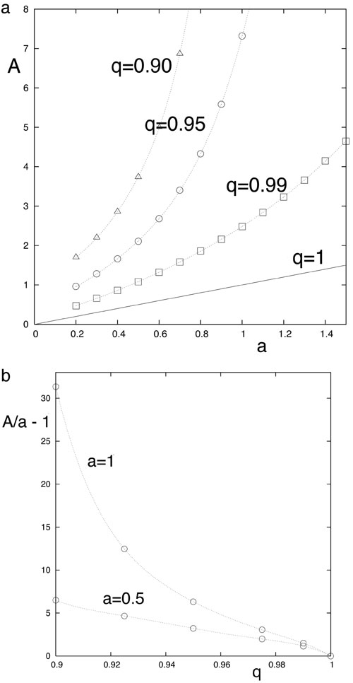
Fig. 16. (a, q)-dependence of A (A = a for q = 1). (a) For typical values of q. (b) For typical values of a.

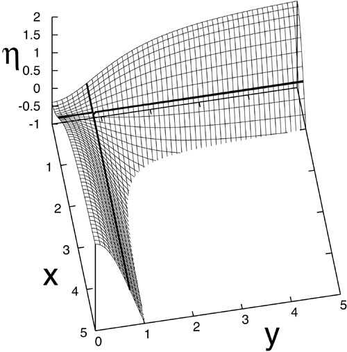
Fig. 17. h(x, y; a, q) for (a, q) = (0.5, 0.95) (hence A = 2.12); x = y is a plane of symmetry, i.e., h(x, y; a, q) = h(y, x; a, q). The two bold straight lines correspond to h = 0.