Supporting Information

Files in this Data Supplement:

Fig. 5. Change in species richness with reserve buying. Change in species richness with conservation investment for three investment strategies as a function of the conservation budget B for varying slopes of supply and demand. Solid diamonds show ecological-economic strategy in which investors have accurate information on species’ distributions and account for impacts on biodiversity in the broader landscape. Gray stars show when investors have accurate information on species’ distributions and acquire sites to maximize coverage of species within the set of purchased reserves. Open circles show when conservation investors lack information on species’ distributions and acquire sites effectively at random. In this figure, no species of conservation concern is assumed able to persist outside reserves, a = 0. Performance is scored against the baseline species richness that would persist with no investment, which in this example is none. Species lists for each site randomly generated while accounting for relative frequency of common and rare species. Discretized supply and demand curves are assumed linear with slopes and intercepts (m_s, p_s) and (m_d, p_d). a and c, shallow/elastic demand (|m_d| = 1/3); b and d, steep/inelastic demand (|m_d| = 3); a and b, shallow/elastic supply (m_s = 1/3); c and d steep/inelastic supply (m_s = 3). Original equilibrium [q₁, p₁] = [50, 50]. Bars show [5, 95] percentiles for n = 200.

Fig. 6. Change in species richness with reserve buying. As for Figs. 3 and 5, but this time a = 1/3 of the species are able to persist on open lands but the remainder can persist only inside reserves.

Fig. 7. Change in species richness with reserve buying. As for Figs. 3 and 5, but this time a = 2/3 of the species are able to persist on open lands but the remainder can only persist inside reserves.

Fig. 8. Optimal allocation of conservation investments across two land markets. The optimal allocation of the conservation budget as a function of the slopes of demand (a) and supply (b) in each land market. All other factors are kept uniform and the two land markets are assumed isolated. In black areas the full conservation budget should be invested in land market 1, and in white areas it should be invested in market 2. All else being equal, land markets in which demand is flatter or supply steeper should be investment priorities. Parameter values: [p_1i, q_1i, B, c_i, A_i, z_i] = [50, 50, 400, 10, 100, 0.3] and in a, M_s = I; b, M_d = –I, where I is the identity matrix.

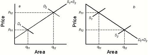
Fig. 9. Comparing the levels of supply and demand in two land markets. (a) The supply of land is the same in each market (S₁ = S₂), but the level of demand is higher in market 2 (D₂). (b) The demand for land is the same (D₁ = D₂), but reservation prices and, hence, the level of supply, are higher in market 1 (S₁). In the absence of conservation buying, the competitive equilibrium in each market is (q_1i, p_1i) for i = 1, 2. In a, biodiversity is most threatened where land is expensive, but in b, it is most threatened where land is cheap. To produce the figure, equal sensitivities of supply and demand were assumed.

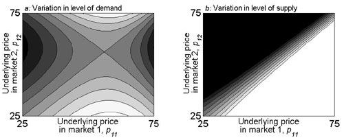
Fig. 10. Optimal allocation of conservation investments across two land markets. The optimal allocation of the conservation budget as a function of the underlying market prices (p₁ = (p₁₁,p₁₂)^T) as the levels of demand (p_di) (a) and levels of supply (p_si) (b) in each land market vary. All other factors are kept uniform, and the two land markets are assumed isolated. In black areas, the full conservation budget should be invested in market 1, and in white areas, it should be invested in market 2. (a) When price changes are induced through demand variation, the optimal allocation is equivocal. (b) When price changes are induced through supply variation, investments should be concentrated in the market where land is cheapest and most threatened. M_d = –I and M_s = I where I is the identity matrix. Other parameter values are [B, c_i,A_i,z_i] = [400, 10, 100, 0.3], and in a, p_si = 0, and in b, p_di = 100.

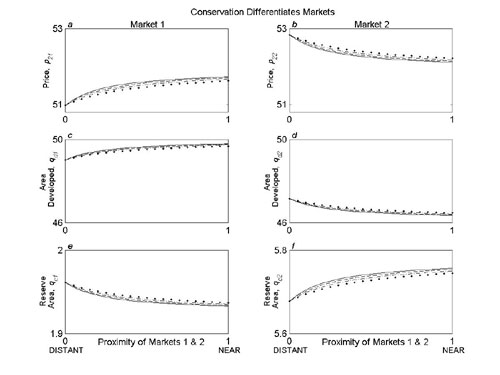
Fig. 11. Effect of given investment allocation across land markets with market differentiation. Effect of proximity (G/min(T_i) = g/4) of land markets (0 is isolated, 1 is near) on market prices p_2i (a and b), the amount of land facing development q_di (c and d), and the amount purchased for conservation q_ci (e and f) in each market for a given budget allocation (B₁, B₂) = (100, 300) when variation in the distribution of reserves differentiates the markets for developers. The solid, dashed, dot-dash, and dotted curves illustrate progressively larger decreases in substitutability from what one would expect based on proximity alone (e= [0, 0.04, 0.08, 0.12], respectively). Baseline levels of supply and demand are given by M_s = I and M_d = –I, where I is the identity matrix, when the land markets are completely isolated (G = g = 0). Other parameter values: [p_1i, q_1i, c_i, A_i, z₁, z₂] = [50, 50, 10, 100, 0.3, 0.31].

Fig. 12. Effect of given investment allocation across land markets with market differentiation when conservation investments create new development opportunities. Effect of proximity (G/min(T_i) = g/4) of the markets (0 is isolated, 1 is near) on market prices p_2i (a and b), the amount of land facing development q_di (c and d), and the amount purchased for conservation q_ci (e and f) in each market for a given budget allocation (B₁,B₂) = (100, 300) when establishing reserves creates new development opportunities and differentiates markets for developers. The solid, dashed, dot-dash, and dotted curves illustrate an increasing impact of reserves in attracting additional development pressure as well as larger decreases in substitutability from what one would expect based on proximity alone (e = [0, 0.04, 0.08, 0.12], respectively, and n = 4e). Baseline levels of supply and demand were given by M_s = I and M_d = –I, where I is the identity matrix, when the land markets are completely isolated (G = g = 0). Other parameter values: [p_1i, q_1i, c_i, A_i, z₁, z₂] = [50, 50, 10, 100, 0.3, 0.31].