A hands-on tutorial on a modeling framework for projections of climate change impacts on health

Abstract

Reliable estimates of future health impacts due to climate change are needed to inform and contribute to the design of efficient adaptation and mitigation strategies. However, projecting health burdens associated to specific environmental stressors is a challenging task, due to the complex risk patterns and inherent uncertainty of future climate scenarios. These assessments involve multi-disciplinary knowledge, requiring expertise in epidemiology, statistics, and climate science, among other subjects. Here, we present a methodologic framework to estimate future health impacts under climate change scenarios based on a defined set of assumptions and advanced statistical techniques developed in time-series analysis in environmental epidemiology. The proposed methodology is illustrated through a step-by-step hands-on tutorial structured in well-defined sections that cover the main methodological steps and essential elements. Each section provides a thorough description of each step, along with a discussion on available analytical options and the rationale on the choices made in the proposed framework. The illustration is complemented with a practical example of study using real-world data and a series of R scripts included as Supplementary Digital Content, which facilitates its replication and extension on other environmental stressors, outcomes, study settings, and projection scenarios. Users should critically assess the potential modeling alternatives and modify the framework and R code to adapt them to their research on health impact projections.

Background

Climate change is one of the most important environmental challenges that humanity will face in the coming decades. Quantifying future health burdens associated with global warming is therefore a major priority for the scientific community, as attested by the increasing number of publications on health impact projections. Several studies have focused on direct impacts of environmental stressors, such as non-optimal temperature and air pollution.^1–5 Generally, these projection studies follow a common methodologic scheme. The basic idea consists in applying risk functions on simulated future exposure distributions generated by climate change models under specific emissions scenarios. However, this scheme entails important methodologic challenges due, for instance, to the complex patterns of health risks associated with environmental stressors, the inherent uncertainty of potential future climate change processes, and the set of (rarely stated) assumptions.⁶ A wide variety of data sources, statistical approaches and assumptions have been applied so far, as summarized and discussed in previous reviews.^6–8 However, a structured illustration that covers the important steps and discuss the most recent statistical developments is still lacking.

Here, we illustrate a methodologic framework to estimate health impact projections under climate change scenarios, built on clearly defined assumptions and state-of-the-art statistical methodologies developed in time-series analysis in environmental epidemiology. This contribution extends a methodology previously presented to project temperature-related excess mortality in climate change scenarios.^5,9 The proposed framework is illustrated through a hands-on tutorial, structured in well-differentiated steps that cover each of the methodologic issues and the essential elements. Each section provides a detailed description of the methodology and a discussion on the potential assumptions and limitations, compared to other available choices. The text is complemented with a practical illustration of a projection study using real-world data, and a series of R scripts included as Supplementary Digital Content, with updated versions available in the personal website and GitHub repository of the last author. The methodologic framework and R code can be modified and adapted to a broad range of health impact projection studies, optionally assessing different environmental stressors and health outcomes, and with different study settings.

Illustrative example

The practical example consists of a projection study on temperature-related mortality impacts in the city of London, United Kingdom. The dataset includes observed daily mean temperature and total number of deaths in London between 1990 and 2012. This is part of the large database collected within the Multi-City Multi-Country (MCC) network (http://mccstudy.lshtm.ac.uk/), and has been previously used as example in other manuscripts.¹⁰ We complement these observed data with daily-modeled temperature series for historical (1950-2005) and future (2006-2100) periods, projected under scenarios defined within the Coupled Model Intercomparison Project Phase 5 of Intergovernmental Panel on Climate Change (IPCC).¹¹ Climate data was obtained, processed and made available by the Inter-Sectoral Impact Model Intercomparison Project (ISI-MIP, https://www.isimip.org/).¹² Further details on the modeled data is provided in the Section 2 of the tutorial.

Tutorial on the modeling framework

1. Estimation of exposure–response associations

One critical step in health impact projection studies is to appropriately define the relationship between the exposure to the environmental stressor of interest and the health outcome. While this information can be based on association estimates reported in the literature,^13,14 this often requires strong assumptions due to extrapolation across geographic areas, and simplification of usually complex relationships.

A more appropriate approach is to directly estimate the relationship using actual epidemiologic data, for which several statistical methods are available.^15,16 Among these, time series analysis using aggregated data has been shown to be ideal to assess short-term associations in environmental epidemiology,¹⁷ and often applied in climate change projection studies.^1,18,19

A representation of the standard time series regression model is provided by the following equation:

$$\text{log}\left[E\left(Y_t\right)\right]=\alpha +f\left(x_t;\mathit{\theta }\right)+s\left(t;\mathit{\beta }\right)+{\displaystyle {\mathit{\sum }}_{p=1}^p{h}_p\left(z_{pt};{\mathit{\gamma }}_p\right)}$$ (1)

where typically the outcome Y_t corresponds to daily counts assumed to follow a Poisson distribution with overdispersion, the function f(x_t; θ) specifies the association with the environmental exposure of interest x at time t, s(t, β) represents the baseline trend which captures the effect of confounders changing slowly over time (i.e., seasonal and long-term trends), and h_p(z_pt; γ_p) models the contribution of other confounders varying on a daily basis.

The exposure–response association can be modeled using different types of function f, ranging from simple indicators for extreme exposure events, to linear or linear-threshold shapes, to distributed lag non-linear models representing complex exposure–lag–response surfaces.²⁰ The selection of the function depends on the environmental stressor, for instance measured as a continuous exposure (e.g., temperature, rain fall) or defined extreme event (e.g., heat wave, floods), and the assumed dependency with the health outcome. As shown below, wrong assumptions on the shape of the dependency can introduce important biases in estimates and projections.

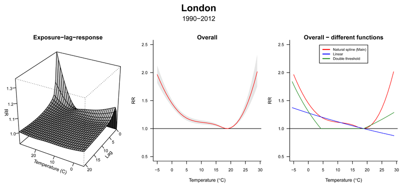
In our example, the environmental stressor and the outcome corresponds to historical series of daily mean temperature and death counts (T_obs and D_obs). Our main choice for the exposure–response function f(x_t) is represented by a distributed lag non-linear model through a bi-dimensional cross-basis term, using flexible natural cubic spline functions to model both exposure–response and lagged-response dimensions, accounting for 21 days of lag, following previous work.¹⁰ As further described in Section 4 of this tutorial, the choice of natural splines allows the log-linear extrapolation of the function beyond the boundaries of the observed series, a step needed to project the risk using the modeled temperature. Figure 1A shows the resulting 3-D plot of the estimated exposure–lag–response association, and Figure 1B represents the overall cumulative exposure–response association across up to 21 days of lag. As expected, we observe a non-linear temperature–mortality relationship, with increases in relative risk (RR) above and below the minimum mortality temperature (T_mm) that correspond to heat and cold associations, respectively. At the same time, risks are distributed differently across time, with immediate heat-mortality and more delayed cold-mortality associations (Figure 1A).

Figure 1. Temperature-related mortality in London (1990-2012).

Left panel: three-dimensional plot showing the estimated exposure–lag–response association between temperature and mortality. Mid panel: overall cumulative mortality risk (and 95% confidence interval). Right panel: comparison between the exposure–response shapes estimated using three modeling approaches.

Alternative models with different specifications of the exposure–response association, such as linear or double-threshold parameterizations, are shown in Figure 1C. While simpler, these choices seem less ideal for modeling the mortality risk of non-optimal temperature, highlighting the importance of the selection of suitable functions to represent the association of interest, and the potential bias of inappropriate simplifications.

2. Projected exposure and health outcome series

Two additional essential elements needed in health impact projection studies are the information on future climatic and population scenarios.

Data on future distribution of the environmental stressor (e.g., temperature, precipitation, air pollution levels) are commonly based on specific scenarios that account for changes in multiple and often inter-related factors. For instance, socioeconomic and technological changes, population growth, and land use changes can affect pathways of greenhouse gases emissions or atmospheric concentrations of other pollutants, which in turn will determine trends in global warming and potential levels of specific environmental exposures.²¹ Under each scenario, these trends can be generated from general circulation models, which offer projections of future conditions based on specific and simplified assumptions.²¹ To have a better representation of future trends, the usual approach is to combine impact estimates obtained either using more than one model per scenario or using ensemble members output from multiple runs of the same climate model, but with different initial conditions. ^6,7

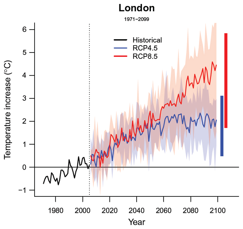
In our worked example, we applied the first approach by including modeled temperature data from five different general circulation models for two climate change scenarios, defined as representative concentration pathways 4.5 and 8.5 (RCP4.5 and RCP8.5).^22,23 Figure 2 shows the temporal trends in temperature for the historical (1971-2005) and future (2006-2100) periods projected in London under the two scenarios, depicted as general circulation model-ensemble averages (solid lines) and associated variability (shaded areas). As discussed later in Section 6, the availability of exposure trends from multiple models can be used to determine the related uncertainty of the projected health impacts.

Figure 2. Temporal trends in projected temperature in London (1971 - 2099).

Solid lines correspond to the mean annual temperature estimated across the 5 GCMs-specific modeled series. The shaded area shows its variability, corresponding to the range for each year. The two horizontal bars in the right correspond to the average annual maximum and minimum for each modeled temperature series.

Projection exercises also depend on representations of future mortality trends, determined by the demographic structure and outcome baseline rates. Data on these population scenarios can be built following different approaches based on the adopted assumptions. The simplest procedure consists in assuming that populations and outcome rates will remain constant in the future, thus isolating the climate effect from other important trends.^24–26 However, other studies relied on population projections derived from predictive models under varying levels of future fertility, mortality, and migration,^27–29 a procedure that requires additional assumptions.

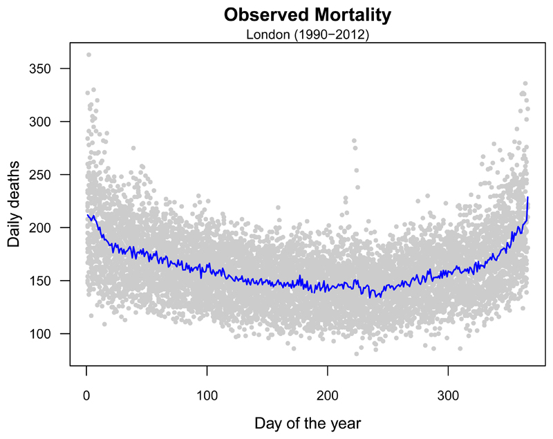
In our example, we illustrate an application of the former method. First, we compute an annual series of total mortality counts as the average for each day of the year from observed daily deaths, thus keeping into account the seasonal structure of the observed mortality series (Figure 3). The annual series is then replicated along the whole projection period. The extension to more complex scenarios requires the derivation of age-specific mortality series, obtained using projection methods that model changes in the demographic structure and baseline rates, as further explained in Section 7 of this tutorial.

Figure 3. Seasonal mortality trends in London.

Grey dots correspond to the observed daily mortality counts registered in each day of the year between 1990 and 2012. The blue line depicts the mean number of deaths per day of the year.

3. Downscaling and calibration

Climate simulations of historical periods usually show systematic deviations from the real-world observations. This can be explained by real differences due to the different geographical resolution of the data (gridded versus point-source), or to biases due to poor performance of climate models, occurring in areas with sparse information from meteorological stations. These deviations should be carefully considered in climate change projection studies, as the predicted impacts will depend on the alignment of observed and modeled series.^30,31 Corrections of biases related to these two aspects have been defined separately as downscaling and calibration, although in most cases they rely on similar analytic procedures. Downscaling refers to the process of obtaining location-specific climate information from global or regional models that provide data at a larger geographic resolution, and is based on either dynamic or statistical methods.⁷ Conversely, calibration is a more general concept of re-aligning two series of data, in this case observed and modeled series.

Bias correction methods have been proposed for both statistical downscaling and calibration, and encompass various different techniques with varying degree of complexity, ranging from basic statistical approaches (i.e., use of additive or multiplicative corrections, shifted distribution), to more complex statistical procedures.³¹ However, limited evidence exists about the potential impact of the choice of method on the estimated projections.

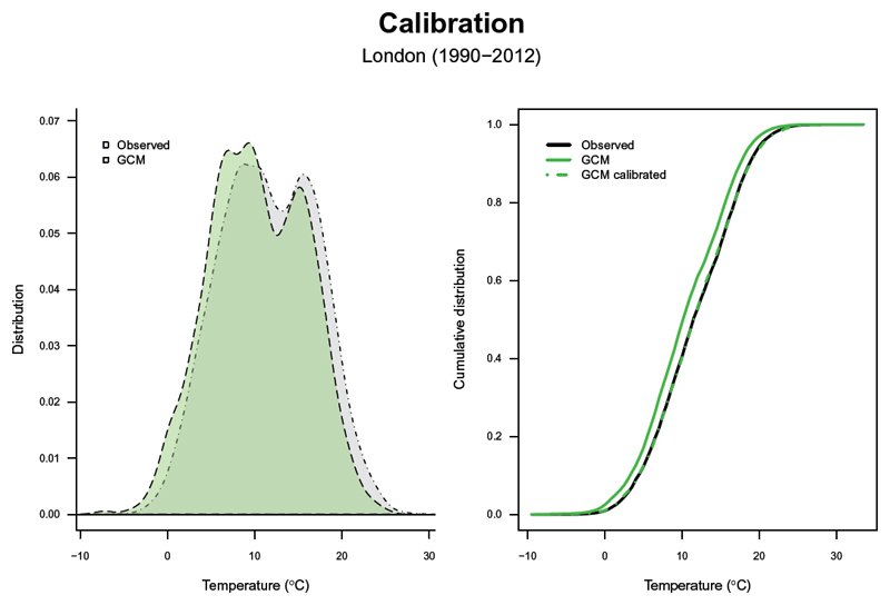
In the present tutorial, the model outputs from the general circulation models are first downscaled through bi-linear interpolation at a 0.5°×0.5° spatial resolution and linearly interpolated by day of the year. The resulting series are then calibrated with the observed data using the bias-correction method developed within ISI-MIP.³² This ensures that the trend and variability of the original data are preserved by adjusting the cumulative distribution of the simulated data to the observed one. In detail, the monthly variability and mean are corrected only using a constant offset or multiplicative correction factor that corrects for long-term differences between the simulated and observed monthly mean data in the historical period.³² Figure 4 shows a comparison between the modeled series from a specific general circulation model (T_mod, green area and line), and the observed series (T_obs, black area and line), in terms of their overall and cumulative distribution (left and right panels, respectively). It can be noted that the modeled series is shifted towards colder ranges, likely for the reasons mentioned above. As discussed, this would create a bias in the future projections. The bias-correction procedure described above calibrates the modeled series ($T_{\mathit{\text{mod}}}^{*}$, green dashed line), re-aligning it to the observed one (Figure 4, right panel).

Figure 4. Bias-correction of the modeled temperature series.

Comparison between the distribution (left panel) and cumulative distribution (right panel) of the raw and bias-corrected modeled temperature(T_mod, $T_{\mathit{\text{mod}}}^{*}$), and the observed temperature series (T_obs). GCM indicates general circulation model.

4. Extrapolation of exposure–response curves

Risk estimates obtained over historical periods do not automatically apply to future scenarios, due to several reasons. For instance, it is possible that the estimated exposure–response association will be different in the future, due to for example adaptation or changes in vulnerability of the population. However, even when assuming no changes in risk, the future distribution of a specific environmental stressor is likely to be different from that observed in the present days and can extend further than the region of the estimated exposure–response curve. Thus, we need to perform an additional step consisting in the extrapolation of the exposure–response beyond the observed boundaries. This, however, implies the adoption of additional assumptions on the hypothetical shape of the association over the unobserved range.

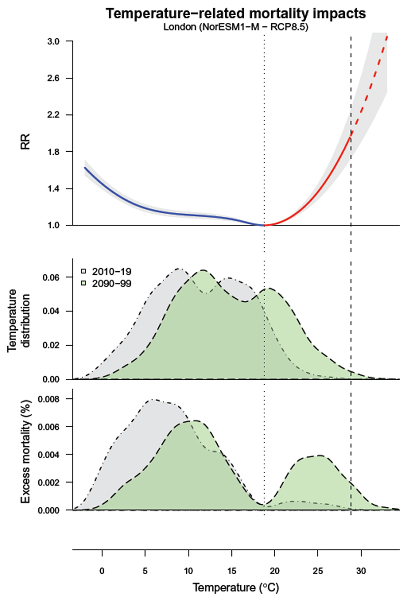
As shown in Figure 5 (top panel), a viable method is based on a log-linear extrapolation of the curve beyond the observed boundaries. The use of a natural cubic spline function to model the exposure–response dimension ensures this non-linear extrapolation, although this step can be more problematic when applying different functions. Nonetheless, this entails a series of strong assumptions on the future risk associated to environmental factors. The first assumption, mentioned above, is that the exposure–response association estimated on the currently observed range will not change in the future, for instance as a result of changes in susceptibility of the population, as discussed in Section 7. The second assumption is that the extrapolation represents appropriately the risk over the unobserved range. In addition, due to the nature of the epidemiologic approaches, the extrapolation of the curve over un-observed ranges constitutes an important source of uncertainty to our projection estimates. This last issue will be further described in Section 6.

Figure 5. Temperature and excess mortality in London for present and future periods.

Top panel: exposure–response curve represented as mortality relative risk (RR) across the temperature (°C) range, with 95% empirical confidence intervals (grey area). The dotted vertical line corresponds to the minimum mortality temperature (T_mm) used as reference, which defines the two portions of the curve related to cold and heat (blue and red, respectively). The dashed part of the curve represents the extrapolation beyond the maximum temperature observed in 2010-19 (dashed vertical line). Mid panel: distribution of $T_{\mathit{\text{mod}}}^{*}$ for the current (2010-19, grey area) and at the end of the century (2090-99, green area), projected using a specific climate model (NorESM1−M) and scenario (RCP8.5). Bottom panel: the related distribution of excess mortality, expressed as the fraction of additional deaths (%) attributed to non-optimal temperature compared with T_mm.

5. Projection and quantification of the impact

The next step of the proposed analytical framework consists of estimating the projected health impacts estimates by applying the exposure–response association estimates over the modeled series of the specific environmental stressor and outcome. Previous studies reported measures of impact using various measures, for instance in terms of percent changes in the rate of the outcome, excess mortality or morbidity, or attributable fractions.^5,18,33 Our framework incorporates the procedure previously developed to estimate the impacts in terms of attributable fractions within in time series analysis, applicable either with the distributed lag nonlinear model framework or with simpler exposure–response dependencies.³⁴

In brief, the method consists of computing for each day of the series the number of cases attributed to a specific environmental stressor based on the estimated risk and the level of exposure in that specific day. Then daily attributable numbers are aggregated by defined intervals of time in the future period. It can be also expressed in terms of attributable fraction computed as the ratio with the corresponding total number of cases. Finally, projection studies are mostly interested in obtaining comparative measures of impact between climate change scenarios or timeframes, which can be easily computed as differences in attributable numbers or fractions.

In the specific setting of the example of study, we estimate the attributable number of deaths D_attr due to non-optimal temperatures using the calibrated temperature series $T_{\mathit{\text{mod}}}^{*}$ following:

$$D_{attr}=D·\left(1-e^{-\left(f^{*}\left(T_{\mathit{\text{mod}}}^{*};{\mathit{\theta }}_b^{*}\right)-s^{*}\left(T_{mm};{\mathit{\theta }}_b^{*}\right)\right)}\right)$$ (2)

where f* and θ* represents the uni-dimensional overall cumulative exposure–response curves with reduced lag dimension, derived from the bi-dimensional term estimated in Section 1 of the tutorial. In Eq.2, we can also separate components due to heat and cold by summing the subsets corresponding to days with temperatures higher or lower than T_mm.¹⁰ The same computation can be used with simpler exposure–response functions, and the equation simplifies to the usual (RR-1)/RR in the case of linear or binary unlagged relationships.

The selection of the T_mm is a critical step in the quantification of the attributable mortality. While this step has been shown to have little impact in well-powered multi-location studies relying on best linear unbiased predictions, this choice can be problematic in single-location analyses that can be affected by highly imprecise exposure–response curves.^10,35

Figure 5 (mid and bottom panels) shows the distributions of temperatures and estimated attributable mortality, respectively, for the historic and future period in London under the assumption of stable populations and no changes in vulnerability. We can observe that the mortality burden due to cold temperatures is currently much larger than for heat, especially across the moderate cold temperatures. However, if we compare the estimates between each of the two periods, we can see that heat-attributable mortality will substantially increase in the future by 4.0% (95% empirical confidence interval (eCI): 0.7-6.8), while mortality due to cold will be reduced by 3.3% (95% eCI: 4.3-1.9). A description on the computation of the eCI is provided in the following section. The same methodologic procedure can be applied to derive attributable mortality for more complex scenarios, as illustrated in Section 7.

6. Ensemble estimates and quantification of uncertainty

A key methodologic issue in projection studies is to properly identify and deal with the different sources of uncertainty involved in the projection of impacts in future scenarios. These include those related to purely statistical aspects, such as the imprecision of the estimated exposure–response function, and the inherent uncertainty of the exposure simulations obtained from the climate and circulation models.⁶

Based on the proposed framework, uncertainty arises mainly from two main sources: the estimation of the exposure–response function, especially regarding the range over which we extrapolated the curve, and climate projections. These are represented by the covariance matrix V(θ_b) of the model coefficients estimated in Equation 1 defining the exposure–response function, and the variability of the modeled series generated in each GCM (Figure 2), respectively. In the tutorial, we quantify this uncertainty by generating 1000 samples of the coefficients through Monte Carlo simulations, assuming a multivariate normal distribution for the estimated spline model coefficients, and then generating results for each of the five general circulation models.³⁴ We report the results as point estimates, using the average across climate models (general circulation model ensemble) obtained by the estimated coefficients, and as eCI, defined as the 2.5^th and 97.5^th percentiles of the empirical distribution of the attributable mortality across coefficients samples and general circulation models. These eCIs account for both sources of uncertainty.

As briefly mentioned before, we did not account for additional uncertainty derived from the estimation of T_mm. If desired, it is possible to quantify it using probabilistic methods showed in recent publications.^35,36 Likewise, other sources of uncertainty can arise in more complex projection scenarios, such as those assuming changes in vulnerability (adaptation) and population structure. However, these can be more difficult to integrate quantitatively in the overall estimate of uncertainty.

7. Accounting for complex scenarios: demographic changes and adaptation

The example illustrated so far is built under the assumptions of no-adaptation and stable populations. Findings from this exercise can answer the question: “What will the temperature-related impact be in the future if the current population would be exposed to warmer temperatures projected in the future?”. However, there is a growing interest in assessing environmental impacts under more complex scenarios that account for changes in both future risks and baseline population, which could a priori approximate more realistically future health impacts. This additional section aims at describing these potential extensions.

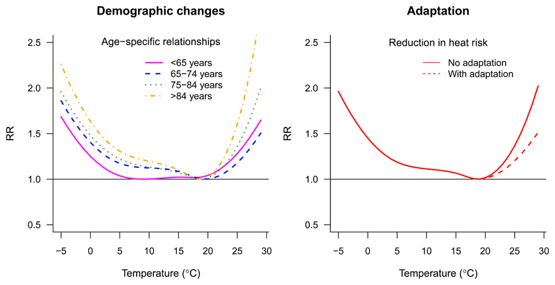
As mentioned before in the Section 2 of the tutorial, changes in size and population structure may have a strong influence on future health impacts, both by increasing the population at risk and by shifting it toward more susceptible groups with higher associated risks. Some studies have accounted for this using age-specific risks and outcome rates derived from socio-economic trajectories,^18,19,27,37 defined for example in the so-called shared socio-economic pathways.³⁸ This can be incorporated in this framework by replicating the proposed procedure by each age category. This step requires the estimation of age-specific exposure–response associations, as shown in Figure 6A, and their application over the corresponding future age-specific outcome series built under a specific shared socio-economic pathway. These modeled outcome series can be derived by re-scaling the observed seasonal counts in the current period using age-specific baseline populations and rates projected in the future under a specific shared socio-economic pathway. However, it should be noted that, while the “stable populations” approach is built on simplistic assumptions and cannot provide a realistic representation of future excess burdens, it offers a more straightforward interpretation as it separates the impact of global warming from other changes, such as those related to demographic variations, that would occur anyway even in a stable climate.

Figure 6. Accounting for complex scenarios accounting for socio-demographic changes and adaptation.

Right panel: age-specific exposure–response curves, applicable to project health impact separately for each age category, thus potentially accounting for demographic changes by using differential baseline mortality trends. Left panel: comparison between the exposure–response curves under scenarios of no adaptation (continuous line) and adaptation (dashed line), the latter under the (simplistic) assumption of an hypothetical attenuation of 30% in risk associated to heat.

Another important issue to be considered in health projection studies is the potential changes in susceptibility to specific environmental stressors. For example, evidence obtained so far indicates that populations have partly adapted to heat stress in the last decades, with related risks showing an attenuation along this period.³⁹ Under these assumptions, exposure–response associations obtained on historical data would not be representative of future risks, and several methods have been proposed to address this issue. These include the analogue city approach,^14,40 which makes use of exposure–response estimates from a location with a climate similar to that projected in the future, or methods that allows direct changes in the estimated exposure–response function^41–44 Both approaches can be incorporated into the proposed framework by replacing or modifying the estimated exposure–response function. As an illustrative example, Figure 6B shows the modified temperature–mortality curve for London, assuming a decrease in 30% in the mortality log-RR associated with heat only, obtained by applying a scaling factor to the related part of the curve. However, one should take into account that this approach, while potentially more realistic, often implies simplistic assumptions on the form of the future exposure–response shape and its changes due to adaptation (e.g., linear-threshold shapes, or shifts). In addition, while few studies have used empirical evidence from historical data,⁴³ most of them have defined an arbitrary set of parameters to model the extent and timing of adaptation mechanisms.⁴² A recent publication has discussed problems and limitations of existing methods for modeling adaptation, also showing how the choice greatly influences the estimated health impacts, and discussing the difficulties in defining and quantifying valid adaptation mechanisms.⁴⁵ Thus, further implications on the potential limitations of the applied method should be considered and clearly discussed when assuming hypothetical changes in vulnerability.

Overview and final remarks

In this contribution, we have presented a well-structured and flexible methodologic framework, based on cutting-edge statistical techniques and clearly defined assumptions, to obtain health impact projections under climate change scenarios of variable complexity. Shaped as a hands-on tutorial, this article describes the key methodologic steps through a practical example of an applied analysis, complemented with real data and R code. While the analytical approaches described in the example are tailored to the specific study settings and should not be uncritically applied in a ‘cut-and-paste’ approach, this tutorial offers the reader the opportunity to advance through general methodologic steps, following how different statistical choices and assumptions have been translated in the analysis and code. At the same time, it enables the reader to replicate, adapt, and potentially extend the proposed modeling framework by applying alternative modeling choices using other environmental stressors, outcomes, study settings, and more complex climate change scenarios. In a more general context, this tutorial highlights the need of multi-disciplinary knowledge and skills for projecting health impacts under climate change scenarios, involving experts working in different research areas, such as epidemiology, statistics, and climate science, among other subjects. This contribution clearly advocates for collaborative research and emphasizes the benefits of reproducibility and transparency in science.

Supplementary Material

As Supplementary Digital Content, we provide the data and R code that illustrates the analytical steps described in this contribution and reproduces the figures shown in the main manuscript.

References

- 1.Petkova EP, Vink JK, Horton RM, et al. Towards More Comprehensive Projections of Urban Heat-Related Mortality: Estimates for New York City under Multiple Population, Adaptation, and Climate Scenarios. Environ Health Perspect. 2017;125(1):47–55. doi: 10.1289/EHP166. [DOI] [PMC free article] [PubMed] [Google Scholar]
- 2.Weinberger KR, Haykin L, Eliot MN, Schwartz JD, Gasparrini A, Wellenius GA. Projected temperature-related deaths in ten large U.S. metropolitan areas under different climate change scenarios. Environ Int. 2017;107:196–204. doi: 10.1016/j.envint.2017.07.006. [DOI] [PMC free article] [PubMed] [Google Scholar]
- 3.Stowell JD, Kim Y-M, Gao Y, Fu JS, Chang HH, Liu Y. The impact of climate change and emissions control on future ozone levels: Implications for human health. Environ Int. 2017;108:41–50. doi: 10.1016/j.envint.2017.08.001. [DOI] [PMC free article] [PubMed] [Google Scholar]
- 4.Abel DW, Holloway T, Harkey M, et al. Air-quality-related health impacts from climate change and from adaptation of cooling demand for buildings in the eastern United States: An interdisciplinary modeling study. PLoS Med. 2018;15(7):e1002599. doi: 10.1371/journal.pmed.1002599. [DOI] [PMC free article] [PubMed] [Google Scholar]
- 5.Gasparrini A, Guo Y, Sera F, et al. Projections of temperature-related excess mortality under climate change scenarios. Lancet Planet Health. 2017;1(9):e360–e367. doi: 10.1016/S2542-5196(17)30156-0. [DOI] [PMC free article] [PubMed] [Google Scholar]
- 6.Huang C, Barnett AG, Wang X, Vaneckova P, FitzGerald G, Tong S. Projecting Future Heat-Related Mortality under Climate Change Scenarios: A Systematic Review. Environ Health Perspect. 2011;119(12):1681–1690. doi: 10.1289/ehp.1103456. [DOI] [PMC free article] [PubMed] [Google Scholar]
- 7.Sanderson M, Arbuthnott K, Kovats S, Hajat S, Falloon P. The use of climate information to estimate future mortality from high ambient temperature: A systematic literature review. PLOS ONE. 2017;12(7):e0180369. doi: 10.1371/journal.pone.0180369. [DOI] [PMC free article] [PubMed] [Google Scholar]
- 8.Kinney PL, O’Neill MS, Bell ML, Schwartz J. Approaches for estimating effects of climate change on heat-related deaths: challenges and opportunities. Environ Sci Policy. 2008;11(1):87–96. doi: 10.1016/j.envsci.2007.08.001. [DOI] [Google Scholar]
- 9.Vicedo-Cabrera AM, Guo Y, Sera F, et al. Temperature-related mortality impacts under and beyond Paris Agreement climate change scenarios. Clim Change. 2018 Sep; doi: 10.1007/s10584-018-2274-3. [DOI] [PMC free article] [PubMed] [Google Scholar]
- 10.Gasparrini A, Guo Y, Hashizume M, et al. Mortality risk attributable to high and low ambient temperature: a multicountry observational study. Lancet. 2015 May; doi: 10.1016/S0140-6736(14)62114-0. [DOI] [PMC free article] [PubMed] [Google Scholar]
- 11.Taylor KE, Stouffer RJ, Meehl GA. An Overview of CMIP5 and the Experiment Design. Bull Am Meteorol Soc. 2011;93(4):485–498. doi: 10.1175/BAMS-D-11-00094.1. [DOI] [Google Scholar]
- 12.Warszawski L, Frieler K, Huber V, Piontek F, Serdeczny O, Schewe J. The Inter-Sectoral Impact Model Intercomparison Project (ISI–MIP): Project framework. Proc Natl Acad Sci. 2014;111(9):3228–3232. doi: 10.1073/pnas.1312330110. [DOI] [PMC free article] [PubMed] [Google Scholar]
- 13.Kendrovski V, Baccini M, Martinez GS, Wolf T, Paunovic E, Menne B. Quantifying Projected Heat Mortality Impacts under 21st-Century Warming Conditions for Selected European Countries. Int J Environ Res Public Health. 2017;14(7) doi: 10.3390/ijerph14070729. [DOI] [PMC free article] [PubMed] [Google Scholar]
- 14.Knowlton K, Lynn B, Goldberg RA, et al. Projecting Heat-Related Mortality Impacts Under a Changing Climate in the New York City Region. Am J Public Health. 2007;97(11):2028–2034. doi: 10.2105/AJPH.2006.102947. [DOI] [PMC free article] [PubMed] [Google Scholar]
- 15.Armstrong B. Models for the relationship between ambient temperature and daily mortality. Epidemiol Camb Mass. 2006;17(6):624–631. doi: 10.1097/01.ede.0000239732.50999.8f. [DOI] [PubMed] [Google Scholar]
- 16.Dominici F, Sheppard L, Clyde M. Health Effects of Air Pollution: A Statistical Review. Int Stat Rev. 2003;71:243–276. [Google Scholar]
- 17.Bhaskaran K, Gasparrini A, Hajat S, Smeeth L, Armstrong B. Time series regression studies in environmental epidemiology. Int J Epidemiol. 2013;42(4):1187–1195. doi: 10.1093/ije/dyt092. [DOI] [PMC free article] [PubMed] [Google Scholar]
- 18.Hajat S, Vardoulakis S, Heaviside C, Eggen B. Climate change effects on human health: projections of temperature-related mortality for the UK during the 2020s, 2050s and 2080s. J Epidemiol Community Health. 2014 Feb; doi: 10.1136/jech-2013-202449. [DOI] [PubMed] [Google Scholar]
- 19.Heaviside C, Tsangari H, Paschalidou A, et al. Heat-related mortality in Cyprus for current and future climate scenarios. Sci Total Environ. 2016;569–570:627–633. doi: 10.1016/j.scitotenv.2016.06.138. [DOI] [PubMed] [Google Scholar]
- 20.Gasparrini A. Modeling exposure–lag–response associations with distributed lag non-linear models. Stat Med. 2013 Sep; doi: 10.1002/sim.5963. [DOI] [PMC free article] [PubMed] [Google Scholar]
- 21.IPCC. Climate Change 2007: The Physical Science Basis. Contribution of Working Group I to the Fourth Assessment Report of the Intergovernmental Panel on Climate Change. Cambridge UK and New York USA: IPCC; 2007. [Google Scholar]
- 22.Moss RH, Edmonds JA, Hibbard KA, et al. The next generation of scenarios for climate change research and assessment. Nature. 2010;463(7282):747. doi: 10.1038/nature08823. [DOI] [PubMed] [Google Scholar]
- 23.Moss RH, Nakicenovic N, O’Neill BC. Towards New Scenarios for Analysis of Emissions, Climate Change, Impacts, and Response Strategies. Geneva: IPCC; 2008. [Accessed July 16, 2018]. http://www.ipcc.ch/pdf/supporting-material/expert-meeting-report-scenarios.pdf. [Google Scholar]
- 24.Baccini M, Kosatsky T, Analitis A, et al. Impact of heat on mortality in 15 European cities: attributable deaths under different weather scenarios. J Epidemiol Community Health. 2011;65(1):64–70. doi: 10.1136/jech.2008.085639. [DOI] [PubMed] [Google Scholar]
- 25.Doherty RM, Heal MR, Wilkinson P, et al. Current and future climate- and air pollution-mediated impacts on human health. Environ Health. 2009;8(1):S8. doi: 10.1186/1476-069X-8-S1-S8. [DOI] [PMC free article] [PubMed] [Google Scholar]
- 26.Doyon B, Bélanger D, Gosselin P. The potential impact of climate change on annual and seasonal mortality for three cities in Québec, Canada. Int J Health Geogr. 2008;7:23. doi: 10.1186/1476-072X-7-23. [DOI] [PMC free article] [PubMed] [Google Scholar]
- 27.Ostro B, Barrera-Gómez J, Ballester J, Basagaña X, Sunyer J. The impact of future summer temperature on public health in Barcelona and Catalonia, Spain. Int J Biometeorol. 2012;56(6):1135–1144. doi: 10.1007/s00484-012-0529-7. [DOI] [PubMed] [Google Scholar]
- 28.Peng RD, Bobb JF, Tebaldi C, McDaniel L, Bell ML, Dominici F. Toward a quantitative estimate of future heat wave mortality under global climate change. Environ Health Perspect. 2011;119(5):701–706. doi: 10.1289/ehp.1002430. [DOI] [PMC free article] [PubMed] [Google Scholar]
- 29.Vardoulakis S, Dear K, Hajat S, Heaviside C, Eggen B, McMichael AJ. Comparative assessment of the effects of climate change on heat- and cold-related mortality in the United Kingdom and Australia. Environ Health Perspect. 2014;122(12):1285–1292. doi: 10.1289/ehp.1307524. [DOI] [PMC free article] [PubMed] [Google Scholar]
- 30.Hewitson BC, Daron J, Crane RG, Zermoglio MF, Jack C. Interrogating empirical-statistical downscaling. Clim Change. 2014;122(4):539–554. doi: 10.1007/s10584-013-1021-z. [DOI] [Google Scholar]
- 31.Maraun D. Bias Correcting Climate Change Simulations - a Critical Review. Curr Clim Change Rep. 2016;2(4):211–220. doi: 10.1007/s40641-016-0050-x. [DOI] [Google Scholar]
- 32.Hempel S, Frieler K, Warszawski L, Schewe J, Piontek F. A trend-preserving bias correction – the ISI-MIP approach. Earth Syst Dynam. 2013;4(2):219–236. doi: 10.5194/esd-4-219-2013. [DOI] [Google Scholar]
- 33.Wu J, Zhou Y, Gao Y, et al. Estimation and Uncertainty Analysis of Impacts of Future Heat Waves on Mortality in the Eastern United States. Environ Health Perspect. 2014;122(1):10–16. doi: 10.1289/ehp.1306670. [DOI] [PMC free article] [PubMed] [Google Scholar]
- 34.Gasparrini A, Leone M. Attributable risk from distributed lag models. BMC Med Res Methodol. 2014;14:55. doi: 10.1186/1471-2288-14-55. [DOI] [PMC free article] [PubMed] [Google Scholar]
- 35.Lee W, Kim H, Hwang S, Zanobetti A, Schwartz JD, Chung Y. Monte Carlo simulation-based estimation for the minimum mortality temperature in temperature–mortality association study. BMC Med Res Methodol. 2017;17(1):137. doi: 10.1186/s12874-017-0412-7. [DOI] [PMC free article] [PubMed] [Google Scholar]
- 36.Tobías A, Armstrong B, Gasparrini A. Brief Report: Investigating Uncertainty in the Minimum Mortality Temperature: Methods and Application to 52 Spanish Cities. Epidemiol Camb Mass. 2017;28(1):72–76. doi: 10.1097/EDE.0000000000000567. [DOI] [PMC free article] [PubMed] [Google Scholar]
- 37.Jackson JE, Yost MG, Karr C, et al. Public health impacts of climate change in Washington State: projected mortality risks due to heat events and air pollution. Clim Change. 2010;102(1–2):159–186. doi: 10.1007/s10584-010-9852-3. [DOI] [Google Scholar]
- 38.Riahi K, van Vuuren DP, Kriegler E, et al. The Shared Socioeconomic Pathways and their energy, land use, and greenhouse gas emissions implications: An overview. Glob Environ Change. 2017;42:153–168. doi: 10.1016/j.gloenvcha.2016.05.009. [DOI] [Google Scholar]
- 39.Arbuthnott K, Hajat S, Heaviside C, Vardoulakis S. Changes in population susceptibility to heat and cold over time: assessing adaptation to climate change. Environ Health Glob Access Sci Source. 2016;15(Suppl 1):33. doi: 10.1186/s12940-016-0102-7. [DOI] [PMC free article] [PubMed] [Google Scholar]
- 40.Hayhoe K, Cayan D, Field CB, et al. Emissions pathways, climate change, and impacts on California. Proc Natl Acad Sci. 2004;101(34):12422–12427. doi: 10.1073/pnas.0404500101. [DOI] [PMC free article] [PubMed] [Google Scholar]
- 41.Gosling SN, McGregor GR, Lowe JA. Climate change and heat-related mortality in six cities Part 2: climate model evaluation and projected impacts from changes in the mean and variability of temperature with climate change. Int J Biometeorol. 2009;53(1):31–51. doi: 10.1007/s00484-008-0189-9. [DOI] [PubMed] [Google Scholar]
- 42.Huynen MMTE, Martens P. Climate Change Effects on Heat- and Cold-Related Mortality in the Netherlands: A Scenario-Based Integrated Environmental Health Impact Assessment. Int J Environ Res Public Health. 2015;12(10):13295–13320. doi: 10.3390/ijerph121013295. [DOI] [PMC free article] [PubMed] [Google Scholar]
- 43.Honda Y, Kondo M, McGregor G, et al. Heat-related mortality risk model for climate change impact projection. Environ Health Prev Med. 2014;19(1):56–63. doi: 10.1007/s12199-013-0354-6. [DOI] [PMC free article] [PubMed] [Google Scholar]
- 44.Dessai S. Heat stress and mortality in Lisbon Part II. An assessment of the potential impacts of climate change. Int J Biometeorol. 2003;48(1):37–44. doi: 10.1007/s00484-003-0180-4. [DOI] [PubMed] [Google Scholar]
- 45.Gosling SN, Hondula DM, Bunker A, et al. Adaptation to Climate Change: A Comparative Analysis of Modeling Methods for Heat-Related Mortality. Environ Health Perspect. 2017;125(8):087008. doi: 10.1289/EHP634. [DOI] [PMC free article] [PubMed] [Google Scholar]
Associated Data
This section collects any data citations, data availability statements, or supplementary materials included in this article.