Abstract
Purpose:
There has been burgeoning interest in applying machine learning methods for predicting radiotherapy outcomes. However, the imbalanced ratio of a large number of variables to a limited sample size in radiation oncology constitutes a major challenge. Therefore, dimensionality reduction methods can be a key to success. The study investigates and contrasts the application of traditional machine learning methods and deep learning approaches for outcome modeling in radiotherapy. In particular, new joint architectures based on variational autoencoder (VAE) for dimensionality reduction are presented and their application is demonstrated for the prediction of lung radiation pneumonitis (RP) from a large-scale heterogeneous dataset.
Methods:
A large-scale heterogeneous dataset containing a pool of 230 variables including clinical factors (e.g., dose, KPS, stage) and biomarkers (e.g., single nucleotide polymorphisms (SNPs), cytokines and micro-RNAs) in a population of 106 non-small cell lung cancer (NSCLC) patients who received radiotherapy was used for modeling RP. 22 patients had grade 2 or higher RP. Four methods were investigated, including feature selection (case A) and feature extraction (case B) with traditional machine learning methods, a VAE-MLP joint architecture (case C) with deep learning and lastly, the combination of feature selection and joint-architecture (case D). For feature selection, Random forest (RF), Support Vector Machine (SVM) and multi-layer perceptron (MLP) were implemented to select relevant features. Specifically, each method was run for multiple times to rank features within several cross-validated (CV) resampled sets. A collection of ranking lists were then aggregated by top 5% and Kemeny graph methods to identify the final ranking for prediction. A synthetic minority oversampling technique (SMOTE) was applied to correct for class imbalance during this process. For deep learning, a VAE-MLP joint architecture where a VAE aimed for dimensionality reduction and an MLP aimed for classification was developed. In this architecture, reconstruction loss and prediction loss were combined into a single loss function to realize simultaneous training and weights were assigned to different classes to mitigate class imbalance. To evaluate the prediction performance and conduct comparisons, the area under receiver operating characteristic (ROC) curves (AUCs) were performed for nested CVs for both handcrafted feature selections and the deep learning approach. The significance of differences in AUCs was assessed using the DeLong test of U-statistics.
Results:
An MLP-based method using weight pruning (WP) feature selection yielded the best performance among the different hand-crafted feature selection methods (case A), reaching an AUC of 0.804 (95% CI: 0.761–0.823) with 29 top features. A VAE-MLP joint architecture (case C) achieved a comparable but slightly lower AUC of 0.781 (95% CI: 0.737–0.808) with the size of latent dimension being 2. The combination of handcrafted features (case A) and latent representation (case D) achieved a significant AUC improvement of 0.831 (95% CI: 0.805–0.863) with 22 features (p-value = 0.000642 compared with handcrafted features only (Case A) and p-value=0.000453 compared to VAE alone (Case C)) with an MLP classifier.
Conclusion:
The potential for combination of traditional machine learning methods and deep learning VAE techniques has been demonstrated for dealing with limited datasets in modeling radiotherapy toxicities. Specifically, latent variables from a VAE-MLP joint architecture are able to complement handcrafted features for the prediction of RP and improve prediction over either method alone.
Keywords: radiotherapy outcome modeling, machine learning, feature selection, deep neural networks
I. INTRODUCTION
Accurate prediction of radiotherapy response is an important component of evaluating patients’ treatment options and for providing insights into designing of new personalized treatments and future clinical protocols. Various analytical, statistical and machine learning methods have been applied into radiotherapy treatment outcome models [1].
Modeling normal tissue toxicity [2] is a main limiting factor towards application of promising hypofractionated and dose escalation studies. Originally, radiotherapy response modeling utilized analytical models, which were generally based on simplified understanding of irradiation effects, such as the Lyman-Kutcher-Burman (LKB) model [3, 4], and the critical volume (CV) model [5, 6]. Later, treatment dosimetry along with clinical and biological factors were incorporated into more advanced statistical (data-driven) models [7], making way towards personalized treatment planning. This is particularly important in the case of radiation-induced lung damage [8], which is a complex disease that manifests in up to 30% of thoracic irradiations in the forms of acute inflammatory radiation pneumonitis (RP) and subsequent chronic pulmonary fibrosis [9]. RP is a major obstacle to treatment success with radiotherapy in lung, esophageal and breast cancers. Therefore, it has been an active area for applying advanced machine learning methods. Artificial neural networks have been applied in the prediction of RP [10, 11]. These studies were based on a one-hidden-layer MLP and used dosimetric and clinical variables only. Support vector machines (SVM) [12, 13] were next applied, but their performance required the selection of several hyperparameters, including kernel related parameters and regularization terms. Bayesian networks [14, 15] were recently applied into this area and gained some notable success. However, this requires prior knowledge of variables inter-relationships, which is necessary to constrain the network structure design.
The application of statistical learning techniques to data-driven outcome modeling in radiotherapy is typically confronted with the problem of limited sample size and an ever increasing number of heterogeneous (clinical, dosimetric, and biological) input variables [1]. One approach to alleviate this problem in conventional machine learning is by “selecting” the most relevant features [16], an active area for many years with different categories of methods. Selection methods that are independent of the learning algorithms (e.g., classifiers) are referred to as filtering methods [17]. They select features according to the general measurement of characteristics of a given dataset (e.g., Pearson correlation). These methods act in a univariate manner and often fail to select the optimal subsets that may work well for the learning task under consideration. Alternatively, wrapper methods try to search for an optimal set of features by preparing and evaluating “goodness” of different combinations of features within a learning scheme [17]. For example, in forward selection, one tries to train a model with a subset of features, based on the inferences from the previous model to decide the features to add to the selected set. However, wrapper methods are computationally expensive. To ease this computational cost, a model-based ranking method was adopted here to select such optimal features, in which a predictive model is built to rank the importance of feature relevance, and then a set of top features is selected as candidate for the optimal set. In this study, multilayer perceptron (MLP)-based [18] selection methods including: weight pruning (WP)[19], feature quality index (FQI) [20], feature-based sensitivity of posterior probability (FSPP) [21] were implemented to rank features’ relevance for the prediction of radiation toxicities. MLPs are recognized as the building block for modern deep learning techniques. For comparison purposes, prevalent machine learning methods based on random forest (RF) [22] and support vector machine (SVM)-based methods [23] were also implemented.
In the new era of deep learning, feature selection and classification can be achieved jointly (e.g., convolutional neural network (CNN)). These methods have demonstrated tremendous success when applied to structured homogeneous data problems in various fields, such as image recognition, natural language understanding and artificial intelligence [24–26]. However, applications to unstructured heterogeneous data such as outcome modeling in radiotherapy is yet to be realized. Towards this goal and as an alternative to conventional feature selection or handcrafting, a deep learning data reduction approach is considered based on variational autoencoders (VAEs). A VAE is an unsupervised learning technique, which can learn latent representation from unlabeled data. Unlike original deterministic autoencoders (AEs)[27], a VAE incorporates variational inference to account for uncertainty, potentially working better with scarce data as encountered in radiotherapy outcome models. In this study, joint VAE-MLP architectures were developed where the latent variable learning (i.e., dimensionality reduction) and the prediction tasks were combined and simultaneously trained for the prediction of RP. This deep learning architecture helped avoiding common cumbersome 2-step procedures in current multivariable predictive modeling and improved the prediction performance over the usual individual and separate application of VAE and conventional classifier methods.
II. DATASET AND PATIENT CHARACTERISTICS
We analyzed 106 non-small cell lung cancer (NSCLC) patients treated under IRB approved protocols. Patients’ RP statuses were evaluated by five-grades CTCAE 3.0 [28] based on clinical assessment and imaging. The RP outcome was then converted into RP2 (RP2=1 when RP= 2 or above, RP2=0 otherwise), serving as an indicator of complication of radiation treatment. The patients were treated with 4 different treatment protocols, in which the first and fourth protocols were dose escalation studies that had the total dose increased up to 86 Gy in 30 fractions, the second and third protocols were with standard dose fractionations, had dose up to 74 Gy, 2 Gy per fraction. Known candidate dosimetric features: Mean_lung_dose, Maximum_Lung_Dose, the total lung volume receiving a dose greater than or equal to 5 Gy (V5), 13 Gy (V13) and 20 Gy (V20) were generated from 2 Gy equivalents (EQD2) dose distributions using the linear/quadratic model (with α / β = 4 Gy)[29]. Dose distributions were computed with the AAA dose calculation algorithm by Varian Eclipse treatment planning system. EQD2 were calculated using locally developed software. Data of cytokines, SNPs, and microRNA were also collected as potential predictors. Blood samples obtained at baseline before treatment, after delivering 1/3 and 2/3 of total dose were analyzed for cytokine levels [30]. Pre-treatment blood samples were also used to analyze SNPs [31, 32] and microRNA levels [33]. All those biomarkers were identified from former study of lung cancer or inflammatory disease. A set of 13 clinical factors such as KPS and Stage was also collected as candidates. A description of the dataset is given in [15] and summarized in TABLE. I for completeness.
TABLE I.
Variables considered in RP2 prediction
| Categories | Names |
|---|---|
| Dosimetric Information (5) | Mean_Lung_Dose, Maximum_Lung_Dose, V5, V13, V20 |
| Clinical Factors (13) | Smoking, COPD, Chemo, Gender, Adenocarcinoma, Squamous cell carcinoma Large cell carcinoma, Poorly differentiated carcinomas, Stage, Age, GTV, KPS, Ratio of weight change |
| Cytokines for pre,2-week and 4 week during treatment (30+30+30) | EGF, eotaxin, fractalkine, G-CSF, GM-CSF, IFN-γ, IL-10, IL-12p40, IL-12p70, IL-13, IL-15, IL-17, IL-1, IL-1, IL-1ra, IL-2, IL-4, IL-5, IL-6, IL-7, IL-8, IP-10, MCP-1, MIP-1α, MIP-1β, sCD40L, TGF-α, TNF-α, VEGF, TGF-β1 |
| miRNAs (62) | Let-7a-5p, miR-100–5p, miR-106b-5p, miR-10b-5p, miR-122–5p, miR-124–3p, miR-125b-5p, miR-126–3p, miR-134, miR-143–3p, miR-146a-5p, miR-150–5p, miR-155–5p, miR-17–5p, miR-17–3p, miR-18a-5p, miR-192–5p, miR-195–5p, miR-19a-3p, miR-19b-3p, miR-200b-3p, miR-200c-3p, miR-205–5p, miR-21–5p, miR-210, miR-221–3p, miR-222–3p, miR-223–3p, miR-224–5p, miR-23a-3p, miR-25–3p, miR-27a-3p, miR-296–5p, miR-29a-3p, miR-30d-5p, miR-34a-5p, miR-375, miR-423–5p, miR-574–3p, miR-885–5p, miR-92a-3p, let-7c, miR-10a-5p, miR-128, miR-130b-3p, miR-145–5p, miR-148a-3p, miR-15a-5p, miR-193a-5p, miR-26b-5p, miR-30e-5p, miR-374a-5p, miR-7–5p, miR-103a-3p, miR-15b-5p, miR-191–5p, miR-22–3p, miR-24–3p, miR-26a-5p, miR-20a-5p, miR-93–5p, miR-16–5p |
|
SNPs (60) |
Rs3857979(BMP1), Rs4988044 (ATM), Rs1800587(IL1A), Rs17561(IL1A), Rs2070874(IL4), Rs1801275(IL4R), Rs4073(CXCL8), Rs2234671(CXCR1), Rs1800896(IL10), Rs3135932(IL10RA), Rs1800872(IL10), Rs11556218(IL16), Rs4760259(GLI1), Rs1799983(NOS3), Rs689470(PTGS2), Rs12102171(SMAD3), Rs6494633(SMAD3),Rs4776342(SMAD3),Rs11615(ERCC1), Rs609261(ATM), Rs12906898(SMAD6), Rs7227023(SMAD7), Rs7333607(SMAD9), Rs664143(ATM), Rs4803455(TGFB1), Rs1061622(TNFRSF1B), Rs664677(ATM), Rs20417(PTGS2), Rs373759(ATM), Rs189037(ATM), Rs12456284(SMAD4), Rs1800057(ATM), Rs3212961(ERCC1), Rs3212948(ERCC1), Rs238406(ERCC2), Rs12917(MGMT), Rs17655(ERCC5), Rs1047768(ERCC5), Rs12913975(SMAD6), Rs1805794(NBN), Rs1625895(TP53), Rs1042522(TP53), Rs25489(XRCC1), Rs9293329(XRCC4), Rs1800469(B9D2&TGFB1), Rs2075685(TMEM167A&XRCC4), Rs25487(XRCC1), Rs1800795(IL6), Rs1799796(XRCC3), Rs1800468(B9D2&TGFB1), Rs1478486(XRCC4), Rs2228000(XPC), Rs2228001(XRC), Rs3218384(XRCC2) Rs1799793(ERCC2), Rs1803965(MGMT), Rs2279744(MDM2), Rs2308321(MGMT), Rs3218536(XRCC2), Rs2834167(IL10RB), Rs3212986(ERCC1) |
III. MACHINE LEARNING METHODS
Several strategies for building multivariable predictive models were investigated here as summarized in FIG. 1. For conventional machine learning, feature selection (case A) and feature extraction (case B) were implemented separately for the classifiers (MLP, SVM, RF). For deep learning, a joint network architecture composed of a VAE and an MLP was implemented for accomplishing feature extraction and prediction tasks simultaneously (case C). Finally, handcrafted features and latent variables from the joint architecture were combined for RP2 prediction (case D).
FIG. 1.
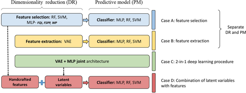
Building multivariable predictive models via standard machine learning and deep architectures
We implemented our models in the Python machine learning package Scikit-learn [34] (RF, SVM) and deep learning package Keras [35]. Specifically, MLP classifiers and VAEs were implemented with Keras sequential model, while VAE-MLP joint architectures were implemented with Keras multi-output models where two losses were combined. All experiments were run on a NVIDIA K40 GPU in the Advanced Research Computing -Technology Services (ARC-TS), FLUX, at University of Michigan.
A. Model-based feature selection techniques
1. MLP-based feature selection methods
An MLP [18] is also called feedforward artificial neural network, which consists of many neurons and several layers where neurons connect to one another in the adjacent layers, as shown in FIG. 2. A neuron in the hidden layer and output layer transforms values from the previous layer into a weighted linear sum followed by a non-linear activation function as shown in Figure FIG. 3. Specifically, ith neuron in the first hidden layer can be calculated as:
| (1) |
where denote the weights and bias, (I1, …, Im) ∈ Rm is an input vector of data and f (·) is the designated activation function. Specifically in this study, sigmoid activation functions were used in hidden layers and a softmax activation function was implemented in the output layer for classification purpose:
| (2) |
A cross-entropy loss function was applied for the discretized classification purpose, where it takes the form
| (3) |
and is optimized using Adam [36] algorithm, an advanced gradient-based optimization algorithm prevalently adopted in deep learning. In Eq. 3, α ∈ {1, 2, … N } is the index of sample, I is the indicator function, y(α) denotes the label for sample α, and denotes the 2-dimensional output vector, which indicates the probability of “yes” and “no” for a given radiation outcome. Note that and , as softmax activation Eq. (2) was applied. The topology of the MLP applied is shown in FIG. 2, with the number of associated nodes shown below layer. Optimal dropout rate was searched among (0.1, 0.2, 0.3, 0.4) on the training set.
FIG. 2.
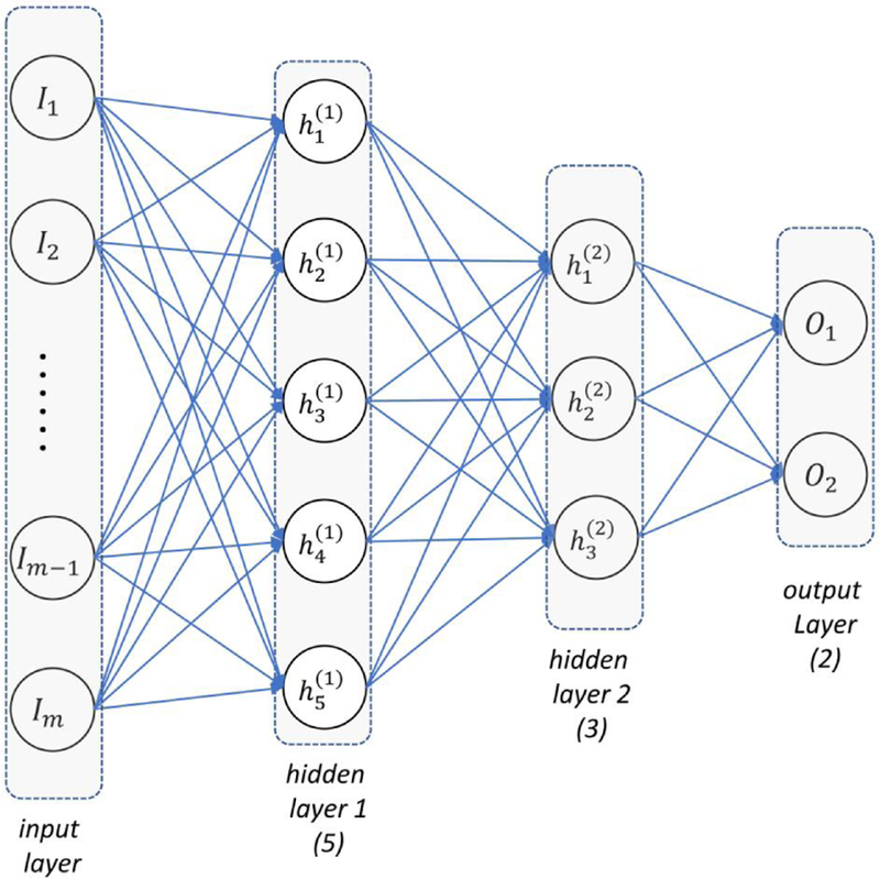
Diagram of MLP: input (I), hidden (h) and output (o) layers are labeled correspondingly. Numbers of nodes are scribed beneath
FIG. 3.
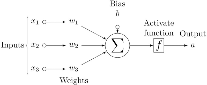
Diagram of a single neuron with 3 input nodes, where an activation function f is applied for final output. (x and a are input and output of this neuron respectively)
Three common techniques for neural networks feature selection are considered here.
Weight pruning (WP) [19]: WP exploits both the weight value and the network structure of a neural network (MLP). The score of ith features, i = 1,…, m, is calculated by summing up the products of weights over all the paths from feature i to outputs. Specifically, in the single-hidden-layer MLP, the importance is written as follows:
| (4) |
where denote the nodes in the input, hidden and the output layer respectively. Eq. (4) suggests the weights to be normalized by the sum of weights that are connected to the same input for comparison reason. WP is based on the intuition that important features should result in weights of relatively large magnitude.
Feature Quality Index (FQI): FQI considers the increase of training mean-squared error (MSE) when a feature is replaced by mean (0 if features are centered). It fixes the trained neural network architecture, and replaces the value of a feature by 0, then, calculates MSE based on the output of a new feature matrix.
| (5) |
where Io are the original features, I(i) is Io with ith feature set to be zero and is the jth output of input matrix of sample α, I(α).
Feature-based Sensitivity of Posterior Probability (FSPP): FSPP considers the variation of outputs when a feature is randomly permuted among samples. One randomly permutes the ith feature among N samples and feeds modified features to the MLP, then calculates the sum of pairwise differences between the new outputs and the original ones. It is based on the belief that “turning off” more important features will influence outputs more.
| (6) |
is the jth output of I(α) after Ii is randomly permuted among N samples.
2. RF and SVM-based feature selection methods
Random forests (RF) and support vector machine (SVM) are among the most popular conventional machine algorithms for prediction and are described in the following.
RF [22]: RF is an ensemble learning method based on decision trees. A decision tree is a flowchart-like structure where each node represents a “test” on an attribute (feature) splitting samples into different branches, nodes can be then repeatedly applied to test attributes of different branches until decision regarding classification is done by the leaf nodes. During this process, the Gini coefficient is a common measure used to decide a split (i.e., the feature applied, threshold). Naturally, features applied at the upper split influencing more input samples should be deemed important. As a result, one can estimate the importance of a feature by the fraction of samples the feature contributes to [34]. RF randomly selects observations and features to build several decision trees and averages the results to reduce the variance. In RF, similarly, one can estimate feature importance by averaging the estimations of feature importance in trees [34]. In RF classifiers, max depth was searched among 2–15 on the training set.
SVM [23]: SVM is an discriminative classifier which can decide an optimal separating hyperplane to categorize samples. In practice, as it is usually not feasible to completely separate samples from different classes, some tolerance errors ϵ are allowed. Mathematically, the optimization problem can be formulated as minimizing the following loss function:
| (7) |
with constraints,
| (8) |
where i is the index for samples, w is a vector parameters to be optimized and φ(·) is a mapping function, which maps variables from an original space usually to a higher dimension space for a better separation. By converting the above optimization problem into a dual optimization problem, the SVM classifier can be represented by:
| (9) |
which can be resolved by solving a convex optimization problem over α = (α1, α2 … α s). K(x, y) is called a kernel function, which corresponds to an inner product in a feature space based on mapping function φ(·). Some common ones are linear, polynomial and radial basis function (RBF) kernels. In the case of linear kernels, parameter w in the original optimization can be easily recovered and used as an estimator of feature importance. RBF-SVM classifiers were implemented with grid search for optimal C (penalty strength) and σ (standard deviation in RBF) among 10 points uniformly distributed in logscale between 0.001 and 1000.
B. Latent variable learning by VAE
1. Variational autoencoder(VAE)
An autoencoder (AE) [37] is an artificial neural network designed for unsupervised learning. It is also used for representation learning [38] where latent variables of input data are learned by attempting to recover its input from them. An AE consists of two parts: an encoder (φ) which compresses an input (from ) into a lower dimensional space (Z) also called latent-space representation, and an decoder (ψ) aiming to reconstruct the input out of the latent-space representation. Mathematically, it is formulated as follows:
Architecture of VAE: layers corresponding to mean µ and standard deviation σ of latent representation z are denoted
| (10) |
where stands for the input space and denotes the latent space. An AE tries to minimize its loss function, which quantifies the reconstruction error (the difference between inputs and outputs) in terms of squared error,
| (11) |
where xenc ∈ denote an input for encoder, xdec := (ψ ◦ φ)(xenc) as an output from decoder, and I is an identity mapping so that one may see from the last expression of Eq. (11) that an AE is in fact attempting to approximate the identity map out of lower dimension. Notice that in the learning process of an AE, no ground truth of data (label) is needed so that it belongs to the unsupervised learning category.
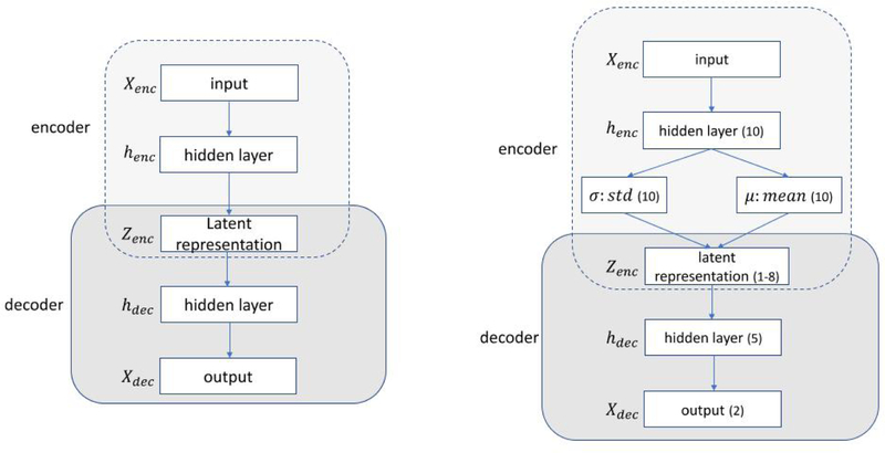
Although autoencoders can be set up by any functional form of φ and ψ, they are typically constructed by neural networks, as shown in FIG. 4 (left). In fact, an AE can be setup by an MLP with at least one hidden layer of smaller dimension (than the input space ) as latent space. Generally, an MLP with an input layer xenc, several hidden layers (henc, zenc, hdec) and an output layer (xdec) whose size is equal to that of the input layer forms an AE.
FIG. 4.
[Left] Diagram of an AE composed of an encoder (E) and a decoder (D). [Right] Diagram of a VAE: numbers of nodes (*) in the implemented architecture are denoted
One notable variant of AE is called a variational autoencoder (VAE) [39], which inherits the AE architecture but incorporates uncertainties through a stochastic variational approach into the deterministic AE. Given inputs xenc, the VAE assumes that the latent representation Z is subject to a Gaussian distribution with mean µ and standard deviation σ rather than a fixed real value. In this setting, the encoder first produces two vectors µ and σ describing the mean and the variance of the latent state distribution and then generates a latent vector by sampling from this distribution. Subsequently, the decoder receives the latent vector to reconstruct the original input.
| (12) |
VAE adopted a method called Variational Inference (VI) which approximates real distribution P (Z|X) by a simple distribution Q(Z|X) (e.g. Gaussian) and then solves it approximately by minimizing a so-called variational lower bound defined as:
| (13) |
where the first term can be approximated by a squared error or cross-entropy loss, and the second term is the Kullback-Leibler divergence metric (also called relative entropy), which has a closed form solution under Gaussian assumptions. Putting all together,one can arrive at [39]
| (14) |
where J is the latent dimension of Z. In the VAE loss Eq. (14), the first term is recognized as the reconstruction error as in Eq. (11) and the second term can be regarded as a regularization term. A VAE was implemented with topology shown in FIG. 4 (right). Its latent output was then fed into various classifiers downstream including MLP, SVM and RF for RP2 prediction.
C. VAE-MLP predictor joint structure
A VAE-MLP “joint” architecture was also implemented for RP2 prediction. A VAE [39] is a unsupervised learning method which aims for representation learning, mapping the original data to a low-dimension latent space. An MLP predictor takes the latent-space representation as input and produces classification decision, i.e, RP2 prediction. The joint-architecture in FIG. 5 conducted dimensionality reduction and prediction tasks simultaneously, realizing efficient representation learning aided by the classification task. The total loss function of the architecture is
| (15) |
where yα is the binary label of data xenc and o is the output prediction for xenc.
FIG. 5.
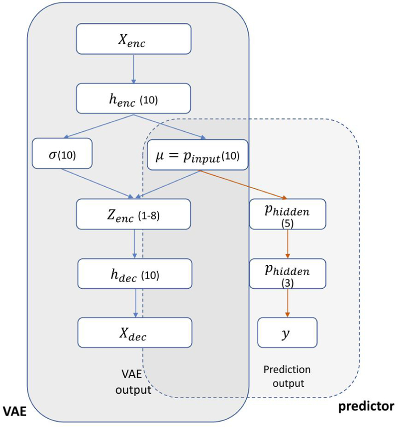
Diagram of a VAE-MLP joint architecture: µ is used as input of MLP classifier. The number of nodes in each layer is given
The first two terms stem from the VAE loss and the third term measures the classification error for the prediction task. The parameter λ in Eq. 15 denotes the trade-off between the two tasks of VAE reconstruction and output prediction. The applied topology of joint architecture is shown in FIG. 5, with λ set as 100 for weighing the magnitude of the two losses.
D. Combining handcrafted features and latent variables
Latent variables from the joint architecture and handcrafted features were combined and fed into RF, SVM and MLP classifiers for RP2 prediction.
IV. ANALYSIS AND PERFORMANCE EVALUATION
We applied wrapper methods [17] based on MLP, RF, SVM to search for the optimal set of features, where the “goodness” of features within each learning scheme was evaluated. Due to the noisy nature of our dataset, the rankings were very sensitive to which portion of the data generated the ranking. As a result, multiple rankings based on different subsets of the data were generated and aggregated to yield a single ranking. Finally, several top features were fed into the designated classifier for evaluation of performance.
For comparison purposes and mitigating statistical bias, we implemented all four methodologies (A, B, C, D in FIG. 1) in the same validation pipeline. This is referred to as a type 2b analysis in the transparent reporting of a multivariable prediction model for individual prognosis or diagnosis (TRIPOD) statement [40]. Specifically, nested CVs were performed, where the feature and parameter selection were tuned in inner-loop CVs, and the model with optimal parameters were then identified from outer-loop training sets and evaluated on outer-loop test sets.
A. Ranking aggregation
To select optimal features, multiple times of inner-loop 5-fold CV were run and the resulting ranking lists based on the training sets were further analyzed for convergence and combined into a single ranking.
The top p% method [41] was applied to aggregate rankings based on different CVs. It uses the frequency of a feature in the top p% as its final score. For example, let p = 5, to get a generalized ranking of m features over c times of 5-fold CVs (with different random seeds for split), one would count how many times feature i appears in the top 5% × m among the 5c ranking lists, and then rank features based on those frequencies, i.e., the higher frequency the feature has, the more important it is.
To decide the cut-off number ĉ of CV times c, we define a deviance value D to evaluate the convergence of ranking lists:
| (16) |
where is the rank of feature i by the bth samples of c times CVs. D(c) is aimed to sum up the deviations of rank (Sci) of all features. We calculated deviations according to resulting ranking lists from B = 100 times of application of the top p% method over a collection of c times CV. Considering features ranking low (with large value Sci) are less important but can affect D(c) equivalently as features ranking high, we divided sample deviations by the mean in D(c). Basically, D quantifies the deviations of orderings given size c and is expected to decrease with increasing of c. One can fix c large enough to make D reasonably small.
After the cut-off number c = ĉ was decided, the top p% methods was applied again to aggregate rankings from 5c ranking lists for B=100 times. Kemeny aggregation [42] was then applied to the resulting 100 ranking lists to reach a final ranking. Kemeny aggregation gets an optimal ranking by minimizing sum of Kendall τ distances, which is defined by the number of pairwise disagreements between any two ranking lists,
| (17) |
with K(τ1, τ2) is the Kendall tau distances of two lists τ1 and τ2:
| (18) |
As one may see, the direct computation of Kemeny aggregation using Eq. (17) and (18) can be burdensome when the lists are long. In fact, it is proven to be an NP-hard problem (at least as hard as nondeterministic-polynomial-time problem). Fortunately, it can be converted into an equivalent graph problem [43] for computational convenience.
Kemeny problem: for B voters (rankings τ1, τ2, … τB ) voting for m candidates (features µ1, … , µm), get the optimal aggregated ranking π.
Equivalent graph problem: every node in the graph represents a candidate (feature). For every pair of candidates i, j, let Q(i > j) denote the number of voters who rank i higher than j. One draws an edge e between each i, j with weight we = |Q(i > j)−Q(j > i)| and orientation from the less preferred to the more preferred node, then solves x in following pure integer linear programming problem as shown by Eq. 19. After optimal x = {xij = 0, 1}, i, j ∈ (1, 2,… m) are obtained, the final ranking list can be deduced, i.e., xij = 1 means i is ranked lower than j in optimal ranking π, xij = 0 means i is ranked higher. The final rank of feature i can be calculated as .
| (19) |
subject to (1) ∀i ≠ j ∈ {1, 2, 3,…, n}, xij + xji = 1,
(2) ∀i ≠ j ≠ k ∈ {1, 2, 3, …, n}, xij + xjk + xki ≥ 1, where x is n × n matrix with binary entries.
B. Validation outline
In the nested CV, outer-loop CVs were performed 10 times to consolidate the results. On outer-loop training sets, single-AUC pre-selection were adopted before application of any dimension reduction method, i.e., only variables with single-variable AUCs > 0.6 were kept and further utilized for feature selection and extraction. This is because when all 200s variables were taken into account, it was too hard to train effective RF, SVM and MLP. Without effective trained models, the derived model-based feature selection can be problematic. Further discussion can be found in SEC. VI.
A synthetic minority oversampling technique SMOTE [44] was adopted to mitigate class imbalance issues for cases A and B. In the VAE-MLP architectures, class imbalance was resolved by setting different weights for the two classes in the prediction loss in Eq. 15. The overall validation process is summarized in FIG. 6.
FIG. 6.
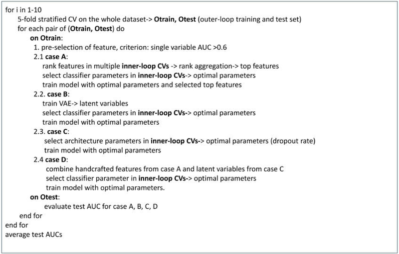
Nested CV in validation process for evaluating for cases A, B, C and D
Delong test [45] which is based on Mann-Whiteney U statistics was performed to conduct comparison of AUCs between different methods. Since Delong test sometimes fails [46] when testing two nested models on the same data that has been used to develop the models, we conducted Delong test only on the test AUCs to alleviate this issue. Delong method was also applied for calculation of CIs of AUCs.
V. RESULTS
A. Conventional machine learning feature selection and prediction (Case A)
Multiple number (c) of inner CVs were performed to rank the features. The cutoff number c = ĉ was decided by the convergence evaluation of the rankings. Then, the top 5% method was applied to the 5ĉ (ĉ times 5-fold CVs) ranking lists for 100 times and further combined into a single ranking by Kemeny aggregation.
Convergence D(c) as defined in SEC. IV A was used to decide ĉ, where c denotes the number of CV being considered in the top 5% method. FIG. 7 shows that D generally decreases with increasing c for all the methods as expected. According to the trends of D, after c = 20, the curve was almost flat, so we fixed c = ĉ (20) in the subsequent experiments.
FIG. 7.
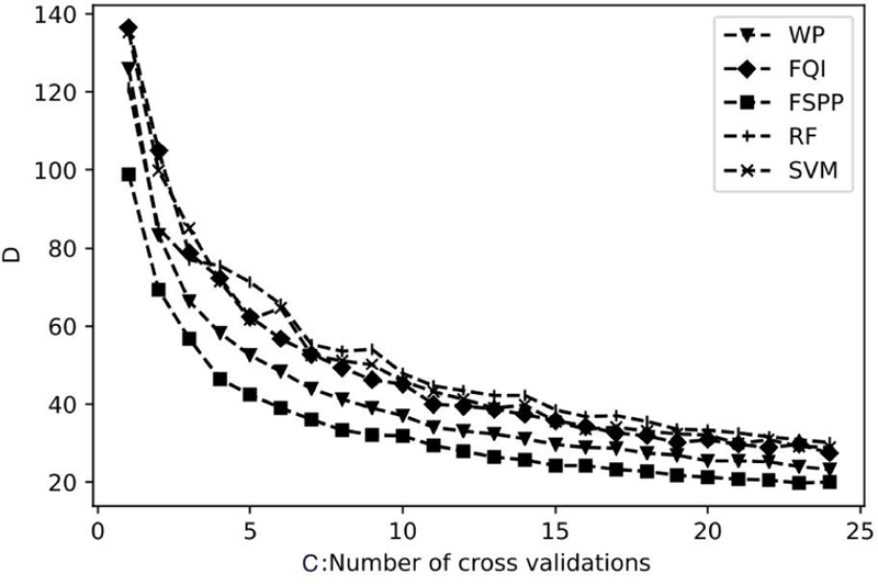
Top 5%: Comparison of convergence (D) as a function of CV size for feature selection methods
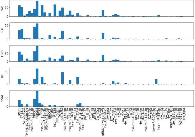
The top 5% criterion was applied to ranking lists from ĉ (20) series of CVs. Frequencies of features being present in the top 5% were counted and served as an overall evaluation of importance. FIG. 8 illustrates an example of frequencies of features based on a random collection of 20 CVs.
FIG. 8.
Top 5%: Frequencies of features based on a random collection of 20 CV
With c being fixed as ĉ (20), the top 5% method was repeated for 100 times and the resulting lists were aggregated by Kemeny optimal aggregation into a generalized ranking, as rankings by the top 5% method from different trials may not be consistent. Specifically, we first calculated the weights of the edges in the defined graph of SEC. IV A based on the 100 ranking lists (as the one derived from FIG. 8) and then solved the deduced integer linear programming problem by python library PuLP [47].
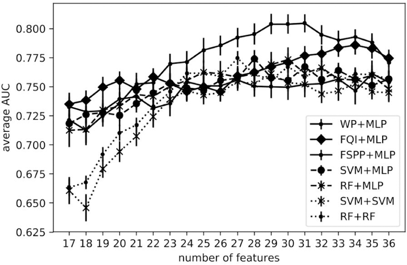
We varied the number of top features included in the predictive models including MLP, RF and SVM according to the final rankings and evaluated their resulting AUCs. To consolidate the results, we repeated the experiment by doing the outer-loop of the nested CVs 10 times. Average test AUCs and their error bars are shown in FIG. 9.
FIG. 9.
Top 5%: AUC trend with increasing number of features
B. VAE analysis with separate and joint classifications (Cases B, C)
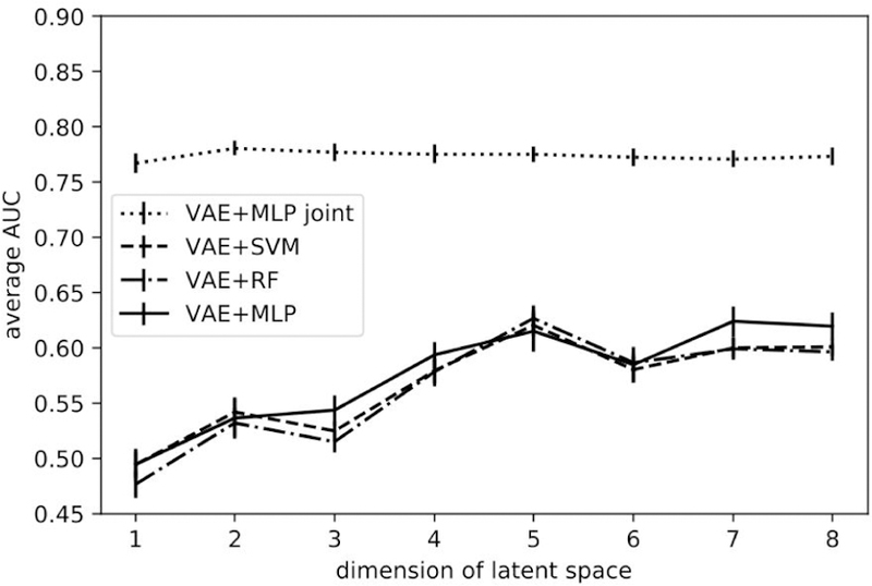
In the VAE-related setting, i.e., cases B & C, all pre-selected features contributed to the prediction task rather than a subset of the selected features as in case A. A comparison of prediction results from case B of separate VAE and classifiers (MLP, SVM, RF) and case C of a VAE-MLP joint architecture is shown in FIG. 10, where the dimension of the latent space varies from 1 to 8. Patients were represented on the 2-D latent space (Z) as points. Examples from some randomly selected outer-loop CVs are shown in Fig. 11.
FIG. 10.
AUC trend with increasing latent dimension
FIG. 11.
Visualization of latent variable Z of patients
C. Combination of handcrafted features and latent variable representation (Case D)
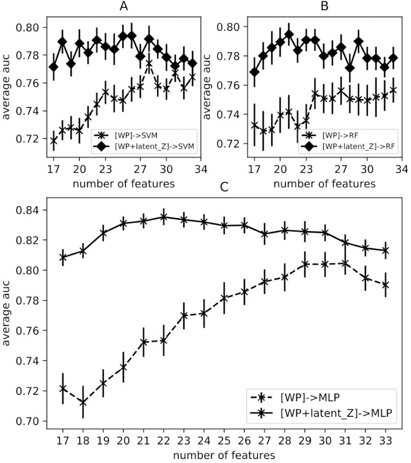
Here, the selected features by WP (case A) and the latent representation from VAE-MLP joint architecture (latent size=2) (case C) were combined and used as inputs in MLP, SVM and RF classifiers for RP2 prediction. The resulting AUCs were shown in FIG. 12, together with AUCs of case A in FIG. 9 for comparison purposes.
FIG. 12.
AUCs by combining WP features with latent_Z in SVM (A) RF (B), MLP (C) classifiers
D. Relevant feature analysis
To analyze feature importance in this study, we considered the final ranking lists in the collection of all (50; 10 times outer-loop CV) iterations. Particularly, the frequency of a feature in the top 29 (the optimal number of features as in FIG. 9) among the all ranking lists was obtained and served as an indicator of relative importance. It turns out that 28 features were selected to be fed into the predictive models more than half of the times, which indicated they were arguably the most relevant features. Merely 7 features (boldface in Table. II) which were selected every time reached a AUC of 0.782 (95% CI: 0.749–0.802) in MLP classifiers for RP2 prediction.
TABLE II.
Features being selected more than half of the times (the boldfaced ones were selected every time) in outer-loop CVs
| Categories | Names |
|---|---|
| Dosimetric Information (1) | Mean_Lung_Dose (α/β=4) |
| cytokine (10) | 2w_eotaxin, 4w_eotaxin, pre_TNF-α, 2w_TNF-α, 4w_TNF-α, 2w_IL-8, 4w_IL-8, 2w_MCP-1, 2w_fractalkine, pre_IFN-γ, |
| miRNA (8) | hsa-miR-192–5p, hsa-miR-22–3p, hsa-miR-128, hsa-miR-15a-5p, hsa-miR-223–3p, hsa-miR-23a-3p, hsam-miR-210, hsa-miR-100–5p |
| SNPs(9) | Rs3857979(BMP1), Rs238406(ERCC2), Rs12456284(SMAD4), Rs1625895(TP53), Rs1799983(NOS3), Rs4803455(TGFB1), Rs25487(XRCC1), Rs1800468(TGFB1), Rs2075685(XRCC4) |
VI. DISCUSSION
In this work, we compared four strategies of building predictive models for lung RP post radiotherapy. Case A and case B both had separate phases of dimensionality reduction and predictive modeling. Particularly, case A adopted dimensionality reduction techniques feature selection (SVM, RF, MLP), and case B adopted feature extraction (VAE). In case C, VAEs and MLP classifiers were trained simultaneously in a deep-learning fashion. Finally, WP handcrafted features (case A) and latent variables (case C) were fed into various classifiers for RP2 prediction in case D.
For case A, RF-, SVM- and MLP-based ranking methods including WP, FQI and FSPP were applied and the top features in the ranking list were used as relevant predictors. Due to the heterogeneity of the data, multiple rankings from several CVs were aggregated into a single ranking list for subsequent prediction task. This can be regarded as an ensemble-like method, analogous to random forest where multiple trees are assembled to make a decision. As shown in FIG. 8, rankings/frequencies by different methods shared some common characteristics, i.e., a few features (e.g., SMAD4, XRCC1) were ranked high by all the methods. Some variations did exist, e.g., mean lung dose (generalized uniform equivalent dose (gEUD)) was ranked high by three MLP-based models but not by RF or SVM. FIG. 9 shows WP+MLP outperformed the rest of the combinations for feature selection and prediction in the range from 23 to 36 features. With top 29 features, WP+MLP was shown to reach highest AUC of 0.804 (95% CI: 0.761–0.823).
In case B and case C, a VAE was implemented for encoding the original inputs. Unlike the common setting as in case B, where VAEs and classifiers were trained subsequently but disjointly for the prediction task, we combined a VAE with a MLP predictor and jointly trained the two parts to improve representation learning in case C. The joint architecture which realized more efficient representation learning with the aid of classification task improved the prediction over the conventional separate training with latent sizes 1 to 8 as shown in FIG. 10. In the joint architecture, two dimensions were sufficient to encode the original inputs for this classification problem, reaching an average AUC of 0.781 (95% CI:0.737–0.808). Two classes RP=0 and RP=1 are clearly separable in training data (red dots versus blue dots) and are partially differentiated in the test data (yellow dots versus green dots) in FIG. 11. Although the joint architectures’ predictive performance is slightly inferior to that of the handcrafted features, it reduces the burdensome feature selection process, statistical bias, and is computationally efficient. In addition, this joint architecture is more data-needy than other proposed selection methods considering its large number of parameters. Therefore, it may potentially work better when more data are made available.
In case D, we considered combining WP handcrafted features and latent variables from VAEs for RP2 prediction. Since case C outperformed case B across all the latent sizes in FIG. 10, we extracted latent variables from the joint architecture only. As shown in FIG. 12, better predictive performance was achieved by combining the selected handcrafted features and the latent representation by VAEs, which is especially in the case of small number of samples. The improvement may be because the latent representation, which takes all features into account to compensate the incomplete discrete representation by the handcrafted feature selection algorithms. When only a small portion of features are available for the predictive model, the complementary information was distinctively useful for such heterogeneous data modeling problem. However, it is our conjecture that, with more data samples become available, case C may supersede handcrafted features to eliminate the necessity of such a combination.
A summary of important results is provided in TABLE. III. For VAE-related methods, Case C outperformed case B with arbitrary latent size. Moreover, combining WP (case A) handcrafted features and latent variables (case D) improved prediction by pure WP features at arbitrary number of features. Note that although we conducted Delong test between case B and case C, case A and case D at specific (the best AUC in each case) points for brevity, the conclusion still held as we varied the number of features/latent sizes as in FIG. 10 and FIG. 12
TABLE III.
Summary of RP2 prediction results from all the 4 strategies
| Methods | Num of features | AUC | Delong test |
|---|---|---|---|
| Case B (VAE+MLP) | 7 (latent_Z) | 0.624 (95%CI: 0.577–0.658) | p-value: 1.33 × 10⁻⁷ |
| Case C (VAE-MLP) | 2 (latent_Z) | 0.781 (95%CI: 0.737–0.808) | |
| Case A (WP+MLP) | 29 | 0.804 (95% CI: 0.761–0.823) | p-value: 6.42 × 10⁻⁴ |
| Case D ([latent Z + WP]+MLP) | 22+2 (latent_Z) | 0.831 (95% CI: 0.805–0.863) |
From TABLE. II, one can see that the reduced feature set from case A was diverse in the type of features, including dosimetric, cytokines, miRNA and SNP variables. This may indicate the necessity of integrating multi-type factors into RP modeling in particular and radiotherapy outcome modeling in general.
In this study, our proposed dimensionality reduction techniques were all applied after pre-processing according to single-variable AUCs, which reduced the number of variables to around 70. This is because our limited sample size is not enough to support application of direct dimension reduction techniques on the original dataset, i.e., the adopted classifiers gave random prediction results without pre-selection. Therefore, such primitive dimensionality reduction by AUC criterion was applied prior to the investigated techniques to mitigate redundancy effects. However, the VAE-MLP joint architecture was still applicable to the whole dataset, though, the predictive performance was degraded even with some additional regularization technique being applied. Particularly, we added a term of L2 regularization to the first-layer weights of the loss function,
| (20) |
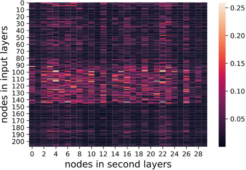
where denote the nodes in first (input) and second layers respectively. The regularization was aimed for sparse weight matrices, addressing the overfitting issue when a large number of features was available. FIGs. 13–15, show heat maps of absolute values of weight parameters in the first layers under different strengths of regularization, where y-axis stands for nodes in the first layer and x-axis denotes the second layer. Clearly, with increasing strength of regularization, weight matrices become sparse and less features take effect in the models.
FIG. 13.
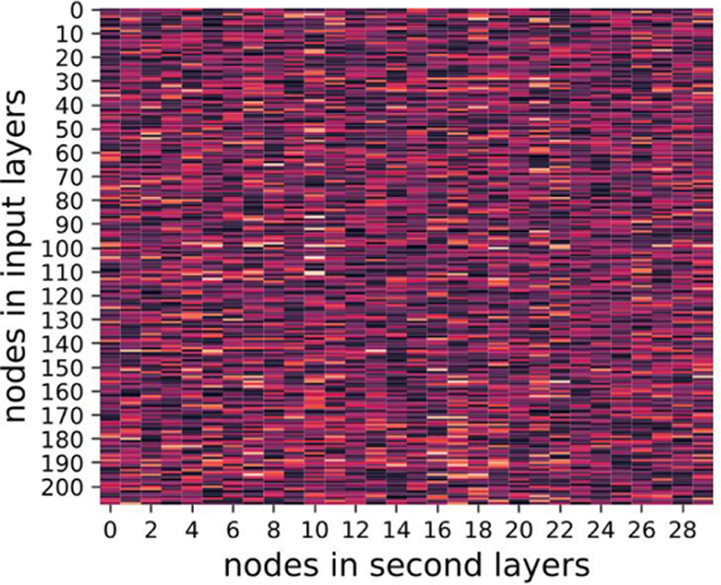
λ = 0.01 visualization of weights
FIG. 15.
λ = 1 visualization of weights
With λ = 1, the average AUC reaches 0.662 (95% CI: 0.622–0.701) outperformed 0.627 at λ = 0. The improved AUC when λ = 1 indicates some random noise in the original data need to be suppressed for better predictive performance.
Without pre-selection, a VAE-MLP joint architecture did not work well even with regularization techniques, which might be due to the fact that the limited sample size was not able to support the rather complex models (too many parameters). One may further consider more advanced VAE structures, which can take into account the correlations between input variables to reduce the demand for sample size, potentially allowing training without such pre-selection. As in the VAE architecture for image data, convolutional neural networks considering spatial invariance and adjacent pixels-correlation take place of the MLP in encoder and decoder architectures. The resulting architecture had far less parameters and required less data to train on. In the outcome modeling data, biological variables which are from the same signaling pathway or longitudinal data measured at different times may be highly correlated with each other, as well as dosimetric data. An advanced VAE architecture considering these inter-correlations may potentially further reduce its dependence on the sample size, enabling better model learning from the raw data.
In this study, we investigated the proposed methods solely on a NSCLC dataset. We recognize that the generalization of this methodology to other datasets is needed. Though modeling outcomes based on such heterogeneous datasets (clinical, dosimetric, imaging, and biomarkers) is recognized to be the right approach, it is still evolving in radiotherapy. As the result, the availability of such dataset is still limited and validation would be the subject of future study. To allow others in the community to explore our approaches, we are currently preparing a Medical Physics DataSet article that will include releasing the data and the associated code.
VII. CONCLUSIONS
This work demonstrates the potential for combination of traditional machine learning methods and deep learning VAE techniques when dealing with limited datasets for modeling radiotherapy toxicities. Specifically, the combination of selected features from MLP-based method WP and latent variables from VAE-MLP joint architecture (case D) yielded the highest AUC compared to the AUCs by either handcrafted features (case A) or latent variables (cases B, C) individually.
FIG. 14.
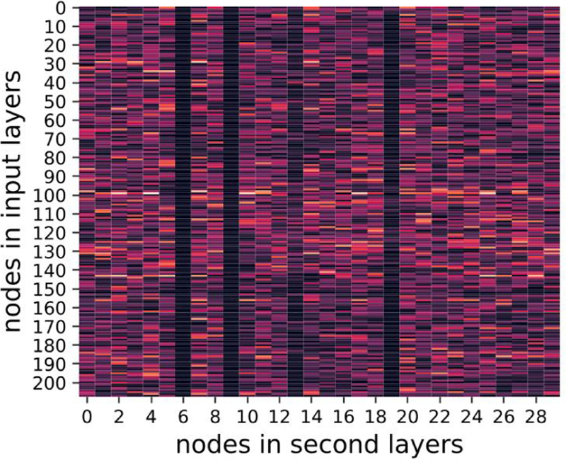
λ = 0.1 visualization of weights
VIII. ACKNOWLEDGMENT
This work was partly supported by National Institutes of Health (NIH) (P01-CA059827 and R37-CA222215) and Rackham Predoctoral fellowship.
Footnotes
The authors have no conflicts to disclose.
References
- [1].El Naqa I, ed., A Guide to Outcome Modeling In Radiotherapy and Oncology: Listening to the Data (2018).
- [2].Bentzen SM, Constine LS, Deasy JO, and et al. , “Quantitative analyses of normal tissue effects in the clinic (QUANTEC): An introduction to the scientific issues,” International Journal of Radiation Oncology Biology Physics 76(3) (2010). [DOI] [PMC free article] [PubMed] [Google Scholar]
- [3].Lyman JT, “Tolerance doses for treatment planning,” (1985), 10.2172/6934260. [DOI] [Google Scholar]
- [4].Kutcher GJ and Burman C, “Calculation of complication probability factors for non-uniform normal tissue irradiation: The effective volume method gerald,” International Journal of Radiation Oncology Biology Physics 16(6), 1623–1630 (1989). [DOI] [PubMed] [Google Scholar]
- [5].Niemierko A and Goitein M, “Modeling of normal tissue response to radiation: The critical volume model,” International Journal of Radiation Oncology Biology Physics 25(1), 135–145 (1993). [DOI] [PubMed] [Google Scholar]
- [6].Stavrev P, Stavrev N, Sharplin J, Fallone BG, and Franko A, “Critical volume model analysis of lung complication data from different strains of mice,” International Journal of Radiation Oncology Biology Physics 81(2), 77–88 (2005). [DOI] [PubMed] [Google Scholar]
- [7].El Naqa I, Suneja G, Lindsay PE, and et al. , “Dose response explorer: an integrated open-source tool for exploring and modelling radiotherapy dose-volume outcome relationships,” Physics in Medicine and Biology 51(22), 5719–5735 (2006). [DOI] [PubMed] [Google Scholar]
- [8].Marks LB, Yorke ED, Jackson A, and et al. , “Use of normal tissue complication probability models in the clinic,” International Journal of Radiation Oncology Biology Physics 76(3), S10–S19 (2010). [DOI] [PMC free article] [PubMed] [Google Scholar]
- [9].Kong FM, Pan C, Eisbruch A, and Ten Haken RK, “Physical models and simpler dosimetric descriptors of radiation late toxicity,” Seminars in radiation oncology fraktur (2007). [DOI] [PubMed]
- [10].Chen S, Zhou S, Zhang J, and et al. , “A neural network model to predict lung radiation-induced pneumonitis,” Medical Physics 34(9), 3420–3427 (2007). [DOI] [PMC free article] [PubMed] [Google Scholar]
- [11].Su M, Miften M, Whiddon C, and et al. , “An artificial neural network for predicting the incidence of radiation pneumonitis,” Medical Physics 32(2), 318–325 (2005). [DOI] [PubMed] [Google Scholar]
- [12].Chen S, Zhou S, Yin F, and et al. , “Investigation of the support vector machine algorithm to predict lung radiation-induced pneumonitis,” Medical Physics 34(10), 3808–3814 (2007). [DOI] [PMC free article] [PubMed] [Google Scholar]
- [13].El Naqa I, Bradley JD, Lindsay PE, Hope AJ, and Deasy JO, “Predicting radiotherapy outcomes using statistical learning techniques,” Physics in Medicine and Biology 54(18), S9 (2009). [DOI] [PMC free article] [PubMed] [Google Scholar]
- [14].Lee S, Ybarra N, Jeyaseelan K, and et al. , “Bayesian network ensemble as a multivariate strategy to predict radiation pneumonitis risk,” Medical Physics 42(5), 2421–2430 (2015). [DOI] [PubMed] [Google Scholar]
- [15].Luo Y, El Naqa I, Mcshan DL, and et al. , “Unraveling biophysical interactions of radiation pneumonitis in non-small-cell lung cancer via bayesian network analysis,” Radiotherapy and Oncology 123(1), 85–92 (2017). [DOI] [PMC free article] [PubMed] [Google Scholar]
- [16].Guyon I and Elisseeff A, “An introduction to variable and feature selection,” J. Mach. Learn. Res 3, 1157–1182 (2003). [Google Scholar]
- [17].Saeys Y, Inza I, and Larranaga P, “A review of feature selection techniques in bioinformatics,” Bioinformatics 23(19), 2507–2517 (2007). [DOI] [PubMed] [Google Scholar]
- [18].LeCun Y, Bengio Y, and Hinton G, “Deep learning,” Nature 521(7553), 436–444 (2015). [DOI] [PubMed] [Google Scholar]
- [19].Yacoub M and Bennani Y, “HVS : A Heuristic for Variable Selection in Multilayer Artificial Neural Network Classifier,” in Intelligent Engineering Systems Through Artificial Neural Networks, edited by Dagli CH (ASME press, 1997) pp. 527–532. [Google Scholar]
- [20].Verikas A and Bacauskiene M, “Feature selection with neural networks,” Pattern Recogn. Lett 23(11), 1323–1335 (2002). [Google Scholar]
- [21].Yang J, Shen K, Ong C, and Li X, “Feature selection for MLP neural network: The use of random permutation of probabilistic outputs,” IEEE Transactions on Neural Network 20, 1911–1922 (2009). [DOI] [PubMed] [Google Scholar]
- [22].Breiman L, “Random forests,” Mach. Learn 45(1), 5–32 (2001). [Google Scholar]
- [23].Tong S and Koller D, “Support vector machine active learning with applications to text classification,” J. Mach. Learn. Res 2, 45–66 (2002). [Google Scholar]
- [24].Krizhevsky A, Sutskever I, and Hinton G, “Imagenet classification with deep convolutional neural networks,” in Advances in Neural Information Processing Systems 25, edited by Pereira F, Burges CJC, Bottou L, and Weinberger KQ (Curran Associates, Inc., 2012) pp. 1097–1105. [Google Scholar]
- [25].Cho K, van Merrienboer B, Gulcehre C, and et al. , “Learning phrase representations using RNN encoder-decoder for statistical machine translation.” in Empirical Methods in Natural Language Processing, edited by Moschitti Alessandro, Pang Bo, and Daelemans Walter (ACL, 2014) pp. 1724–1734.
- [26].Silver D, Huang A, Maddison CJ, and et al. , “Mastering the game of go with deep neural networks and tree search,” Nature 529(7587), 484–489 (2016). [DOI] [PubMed] [Google Scholar]
- [27].Goodfellow I, Bengio Y, and Courville A, “Deep learning research: Autoencoders,” in Deep learning (MIT Press, 2016) http://www.deeplearningbook.org. [Google Scholar]
- [28].Kouloulias V, Zygogianni A, Efstathopoulos E, and et al. , “Suggestion for a new grading scale for radiation induced pneumonitis based on radiological findings of computerized tomography: Correlation with clinical and radiotherapeutic parameters in lung cancer patients,” Asian Pacific Journal of Cancer Prevention 14(5), 2717–2722 (2013). [DOI] [PubMed] [Google Scholar]
- [29].Bentzen SM and Dische S, “Morbidity related to axillary irradiation in the treatment of breast cancer,” Acta Oncologica 39(3), 337–347 (2000). [DOI] [PubMed] [Google Scholar]
- [30].Fukuyama T, Ichiki Y, Yamada S, and et al. , “Cytokine production of lung cancer cell lines: Correlation between their production and the inflammatory/immunological responses both in vivo and in vitro,” Cancer Science 98(7), 1048–1054. [DOI] [PMC free article] [PubMed] [Google Scholar]
- [31].Damaraju S, Murray D, Dufour J, and et al. , “Association of DNA repair and steroid metabolism gene polymorphisms with clinical late toxicity in patients treated with conformal radiotherapy for prostate cancer,” Clinical Cancer Research 12(8), 2545–2554 (2006). [DOI] [PubMed] [Google Scholar]
- [32].Slattery ML, Herrick JS, Lundgreen A, and Wolff RK, “Genetic variation in the TGF-β signaling pathway and colon and rectal cancer risk,” Cancer Epidemiology Biomarkers and Prevention 20(1), 57–69 (2010). [DOI] [PMC free article] [PubMed] [Google Scholar]
- [33].Guo L, Zhang Y, Zhang L, and et al. , “Micrornas,TGF-β signaling, and the inflammatory microenvironment in cancer,” Tumor Biology 37(1), 115–125 (2015). [DOI] [PMC free article] [PubMed] [Google Scholar]
- [34].Pedregosa F, Varoquaux G, Gramfort A, and et al. , “Scikit-learn: Machine learning in Python,” Journal of Machine Learning Research 12, 2825–2830 (2011). [Google Scholar]
- [35].Franc¸ois Chollet, “Keras,” https://keras.io (2015).
- [36].Kingma DP and Ba J, “Adam: A method for stochastic optimization,” CoRR abs/1412.6980 (2014).
- [37].Baldi P, “Autoencoders, unsupervised learning and deep architectures,” in Proceedings of the 2011 International Conference on Unsupervised and Transfer Learning Workshop - Volume 27, UTLW’11 (JMLR.org, 2011) pp. 37–50. [Google Scholar]
- [38].Bengio Y, Courville A, and Vincent P, “Representation learning: A review and new perspectives,” IEEE Trans. Pattern Anal. Mach. Intell 35(8), 1798–1828 (2013). [DOI] [PubMed] [Google Scholar]
- [39].Kingma DP and Welling M, “Auto-encoding variational bayes.” CoRR abs/1312.6114 (2013).
- [40].Collins GS, Reitsma JB, Altman DG, and Moons KG, “Transparent reporting of a multivariable prediction model for individual prognosis or diagnosis (TRIPOD) : the TRIPOD statement,” British Journal of Cancer 112(2), 251–259 (2015). [DOI] [PMC free article] [PubMed] [Google Scholar]
- [41].El Naqa I, Bradley J, Blanco A, and et al. , “Multivariable modeling of radiotherapy outcomes, including dosevolume and clinical factors,” International Journal of Radiation Oncology Biology Physics 64(4), 1275–1286 (2006). [DOI] [PubMed] [Google Scholar]
- [42].Lin S, “Rank aggregation methods,” Wiley Interdisciplinary Reviews: Computational Statistics 2, 555–570 (2010). [Google Scholar]
- [43].Conitzer V, Davenport A, and Kalagnanam J, “Improved bounds for computing kemeny rankings,” in Proceedings of the 21st National Conference on Artificial Intelligence (AAAI Press, 2006) pp. 620–626. [Google Scholar]
- [44].Chawla NV, Bowyer KW, Hall LO, and Kegelmeyer WP, “Smote: Synthetic minority over-sampling technique,” J. Artif. Int. Res 16(1), 321–357 (2002). [Google Scholar]
- [45].Delong ER, Delong DM, and Clarke-Pearson DL, “Comparing the areas under two or more correlated receiver operating characteristic curves: a nonparametric approach,” biometrics 44(3), 837–845 (1988). [PubMed] [Google Scholar]
- [46].Demler OV, Pencina MJ, and D’Agostino RB Sr, “Misuse of DeLong test to compare AUCs for nested models,” Stat. Med 31(23), 2577–2587 (2012). [DOI] [PMC free article] [PubMed] [Google Scholar]
- [47].Mitchell S, Sullivan MO, and Dunning I, “PuLP: A linear programming toolkit for Python,” (2011), http://www.optimization-online.org/DB_FILE/2011/09/3178.pdf.


