Analysis, Modeling, and Simulation of the Accuracy of Continuous Glucose Sensors

Abstract

Background

Continuous glucose monitors (CGMs) collect a detailed time series of consecutive observations of the underlying process of glucose fluctuations. To some extent, however, the high temporal resolution of the data is accompanied by increased probability of error in any single data point. Due to both physiological and technical reasons, the structure of these errors is complex and their analysis is not straightforward. In this article, we describe some of the methods needed to obtain a description of the sensor error that is detailed enough for simulation.

Methods

Data were provided by Abbott Diabetes Care and included two data sets collected by the FreeStyle Navigator™ CGM: The first set consisted of 1032 time series of glucose readings from 136 patients with type 1 diabetes and parallel time series of reference blood glucose (BG) collected via self-monitoring at irregular intervals. The average duration of a time series was 5 days; the total number of sensor-reference data pairs was approximately 20,600. The second data set consisted of 56 time series of glucose readings from 28 patients with type 1 diabetes and a parallel time series of reference BG measured via the YSI 2300 Stat Plus™ analyzer every 15 minutes. The average duration of a time series was 2 days; the total number of sensor-reference data pairs was approximately 7000.

Results

Three sets of results are discussed: analysis of sensor errors with respect to the BG rate of change, mathematical modeling of sensor error patterns and distribution, and computer simulation of sensor errors:

1. Sensor errors depend nonlinearly on the BG rate of change: Errors tend to be positive (high readings) when the BG rate of change is negative and negative (low readings) when the BG rate of change is positive, which is indicative of an underlying time delay. In addition, the sensor noise is non-white (non-Gaussian) and the consecutive sensor errors are highly interdependent.

2. Thus, the modeling of sensor errors is based on a diffusion model of blood-to-interstitial glucose transport, which accounts for the time delay, and a time-series approach, which includes autoregressive moving average (ARMA) noise to account for the interdependence of consecutive sensor errors.

3. Based on modeling, we have developed a computer simulator of sensor errors that includes both generic and sensor-specific error components. A χ² test showed that no significant difference exists between the observed and the simulated distribution of sensor errors and the distribution of errors of the FreeStyle Navigator (p > .46).

Conclusions

CGM accuracy was modeled via diffusion and additive ARMA noise, which allowed for designing a computer simulator of sensor errors. The simulator, a component of a larger simulation platform approved by the Food and Drug Administration in January 2008 for pre-clinical testing of closed-loop strategies, has been successfully applied to in silico testing of closed-loop control algorithms, resulting in an investigational device exemption for closed-loop trials at the University of Virginia.

Introduction

Continuous glucose monitors (CGMs) provide detailed time series of consecutive observations on the underlying process of glucose fluctuations. The feedback of such detailed information to patients with diabetes has been shown to have positive influence on their glycemic control, including reduction in glucose variability, time spent in nocturnal hypoglycemia, time spent in hyperglycemia, and levels of glycosylated hemoglobin.^1–4 However, a number of studies have concluded that, despite eight years of development, the CGM technology continues to face challenges in terms of sensitivity, stability, calibration, and the physiological time lag between blood glucose (BG) and interstitial glucose (IG) concentration.^5–11 Thus, it is frequently concluded that the abundance of information about glucose fluctuations carried by the CGM data stream is to some extent offset by the possibility of sensor errors that exceed in magnitude the errors of the traditional self-monitored blood glucose (SMBG) devices. Such a conclusion, however, is only partially accurate: while the observed error in an isolated CGM data point is indeed generally larger than the error observed in a SMBG data point, the additional information provided by CGM time series allows the application of error-reduction techniques that are unavailable in SMBG devices. For example, deconvolution and other modeling techniques allow for mitigation of certain sensor deviations due to blood-to-interstitial time delay.^12,13

The key to CGM error mitigation is detailed analysis and subsequent mathematical modeling, which allow the understanding of the sources and magnitude of sensor errors. The analytical approach proposed in this manuscript is based on two principles: (i) CGMs assess BG fluctuations indirectly—by measuring the concentration of IG—but are calibrated via self-monitoring to approximate BG; and (ii) CGM data reflect an underlying process in time and therefore are a time series consisting of ordered, in-time, highly interdependent data points. The first principle stipulates that calibration errors would be responsible for a portion of the sensor deviation from reference BG.¹³ Thus, in accuracy studies, the first step of the analysis should be the investigation of calibration errors via simulated recalibration, using all available reference data points. Furthermore, because CGMs operate in the interstitial compartment, which is presumably related to blood via diffusion across the capillary wall, the second step of modeling sensor deviations from BG should be the description of this diffusion process. Models of blood-to-interstitial glucose transport have been proposed and are reasonably well accepted by the scientific community as an approximation of the possible physiological time lag between BG and IG concentration.^14–16 The second principle stipulates that the temporal structure of CGM data is important and should be taken into account by the analysis of CGM errors. In particular, established accuracy measures, such as mean absolute/relative difference, present an incomplete picture of sensor accuracy because these measures judge the proximity between sensor and reference BG at isolated points in time, without taking into account the temporal structure of the data. In other words, a random reshuffling of the sensor-reference data pairs in time will not change these accuracy estimates. Thus, in order to account for the dynamics of sensor errors, higher-order temporal properties need to be investigated. A wide array of modeling techniques is offered by time-series methods, such as autoregression, autocorrelation, and spectral analysis. In this paper we propose the use of an autoregressive moving average (ARMA) model to account for the time dependence of consecutive sensor errors.

Finally, the detailed understanding and modeling of sensor errors allows the next step, their computer simulation. This in turn allows the development of a simulated “sensor”, which is useful for in silico testing of diabetes treatment strategies, such as open- or closed-loop control, under the realistic conditions of imperfect CGM.

Methods

To decompose the sensor errors, we used techniques from linear regression, kernel density estimation, derivative estimation, and time series analysis, each allowing us to access specific characteristics of the sensor/BG discrepancy. We also provided examples of each analysis using data provided by Abbott Diabetes Care (Alameda, CA).

Data Sets

The data used as an example in this paper comes from two different data sets provided by Abbott Diabetes Care:

1. The first data set is a home-use data set containing sensor readings from the FreeStyle Navigator™ taken every 10 minutes in 136 patients, for an average of 40 days (e.g. 8 sensors, 5-day insertions). The data set contains 1062 sensors, totaling approximately 4000 days of recording, with 40,745 irregularly spaced, reference SMBG data points. After elimination of missing data segments and non-functioning sensors, the final data set was composed of 20,660 reference/sensor data pairs.

2. The second data set is smaller but more controlled, in that BG was measured every 15 minutes in clinical settings, using YSI instruments (coefficient of variation = 2%). It contains Navigator sensor readings taken every minute in 28 patients, 2 sensors per patient at different sites, i.e., 56 sensors. After elimination of missing data and non-functioning sensors, the final data set was composed of approximately 7000 data pairs.

A Posteriori Recalibration

To our knowledge, no model-free calibration procedures are available. Therefore, we used the method generally used by sensor producers, i.e., linear/quadratic fitting with time-delay compensation. A posteriori recalibration of the data was performed for each sensor. The major difference between a posteriori and real-time calibration is the availability of all reference BG points; therefore, for a fixed calibration function (the relation between sensor current and BG), a posteriori calibration is optimal in minimizing the sensor readings-reference glucose discrepancy. In this study, a posteriori calibration was performed by linear regression, matching the interpolated sensor readings (if the timing of the reference fell between two readings of the sensor) to the reference measurements. The sum of squares was assessed only at the points of reference measurement. The result of the linear regression was considered to be the recalibrated sensor trace.

Reference Sensor Density and Delay Estimation

Density estimation

Once the sensors were recalibrated, we used kernel density estimation to approximate the distribution of the sensor readings for different glucose references. Each sensor/reference pair is associated with a Gaussian kernel [see Equation (1)] centered about the pair and of predetermined width. More details on the selection of the width and kernel function can be found in Hastie et al.¹⁷ The density was then computed as the weighted sum of all kernels:

$$D\left(s,r\right)=\frac{1}{2\pi \sigma N}{\displaystyle \sum _{i=1}^N{e}^{\frac{-({(s-s_i)}^2+{(r-r_i)}^2)}{2{\sigma }^2}}}$$ (1)

Here N is the number of pairs, s_i is the sensor reading of pair i, r_i is the reference measure of pair i, and σ is the kernel width. This estimation of the density is slightly biased by the fact that negative glucose values do not occur; the bias is reduced by choosing σ to be less than 25% of the smallest reference value.

Therefore the mean sensor reading (s̄) and the mean error (ε̄) for each reference BG was computed using Equation (2).

$$\begin{array}{l}\overline{s}\left(r\right)={\displaystyle \underset{s=0}{\overset{600}{\int }}s\times D\left(s,r\right)\mathit{ds}}\\ \overline{\epsilon }\left(r\right)=\overline{s}\left(r\right)-r\end{array}$$ (2)

Delay estimation

The premise behind our methodology for delay estimation is that if the CGM measurements are delayed, then the sensor error will be dependent on the rate of change of glucose. Therefore, by computing D(s,r) for different ranges of rates of change in glucose (bins), and studying the differences between bins, we can study the delay. To do so we needed to estimate the density in particular bins using Equation (3):

$$\begin{array}{l}{D}_j\left(s,r\right)=\frac{1}{2\pi \sigma N_j}{\displaystyle \sum _{i=1}^N{I}_j\left(\partial s_i\right)e^{\frac{-({(s-s_i)}^2+{(r-r_i)}^2)}{2{\sigma }^2}}}\\ I_j\left(\partial s_i\right)=\{\begin{array}{l}1\text{if}\partial s_i\text{is}\text{in}{\text{bin}}_j\\ 0\text{otherwise}\end{array}\end{array}$$ (3)

To compute a robust rate of change we used sliding linear regression computed for consecutive 20-minute windows.

Estimation and Modeling of the Sensor Error Distribution

As discussed above, CGMs measure glucose in the interstitial fluid while being used to assess BG, which creates a delay. Therefore, the distribution of sensor errors could not be computed directly by using the difference between reference and sensors at the same time points. Since the physiological delay described above is not constant across subjects or within a subject over a long period of time, we synchronized sensor and reference BG using a first-order diffusion model in the calibration equation [Equation (4)].

$$\begin{array}{l}\mathit{CGM}=\alpha .G_I+\beta \\ {\dot{G}}_I=-\frac{1}{\tau }(G_I-G_B)\end{array}$$ (4)

Here G_I and G_B are the interstitial and the blood glucose concentrations, respectively; τ is the diffusion time constant, and α and β are the calibration parameters. Spanning the possible values of τ, we applied the same linear regression technique as before to estimate α and β. The final solution is the set (τ, α, β) which produces the smallest sum of squares. We do not claim that this procedure, derived from the study by Stein et al.,¹⁶ models perfectly the transport of glucose from blood to interstitium nor the functional relationship between electrical current in the sensor and glucose values. However, in the absence of an identifiable model of such a process, we followed the parsimony principle in choosing the simplest available one, i.e., a linear transformation added to a first order, gain 1, diffusion.

Once sensor and reference data were synchronized, we computed the differences between sensor and reference and estimates, and the first four central moments of their empirical distribution: mean, variance, skewness, and kurtosis.

Finally, based on the Johnson family of distributions,¹⁸ we approximated the probability distribution of the sensor error, using a transformation of the normal density.¹⁹

Estimation and Modeling of Sensor Error Time Dependency

Classical time-series techniques were applied to the recalibrated and synchronized sensor signal to determine the time dependency of sensor errors: the autocorrelation function and the partial autocorrelation functions.

The autocorrelation function (ACF) is fairly straight-forward: it is computed as the correlation of an error at time t, with the errors at time t + h, where h = nT, n is an integer, and T is a fixed time interval. (Generally T is set to the time difference between reference measures.) Under weak stationary conditions (the mean and variance of the error do not depend on time) the ACF is only dependent on the lag (h) and not on t, and can be computed using Equation (5).

$$\gamma (h)=\frac{n}{n-h}\frac{{\displaystyle \sum _{i=1}^{n-h}({\epsilon }_i-\overline{\epsilon })({\epsilon }_{i+h}-\overline{\epsilon })}}{{\displaystyle \sum _{i=1}^n{({\epsilon }_i-\overline{\epsilon })}^2}}$$ (5)

The partial autocorrelation function (PACF) can be best described as the correlation between errors at time t and t + h, h = nT, excluding information transmitted through t + T, t + 2T, t + 3T,…, t + (n − 1)T. It is similar to the concept of best linear predictor and is commonly computed using the Durbin-Levinson algorithm.²⁰ For more details on PACF please refer to Brockwell et al.²²

Results

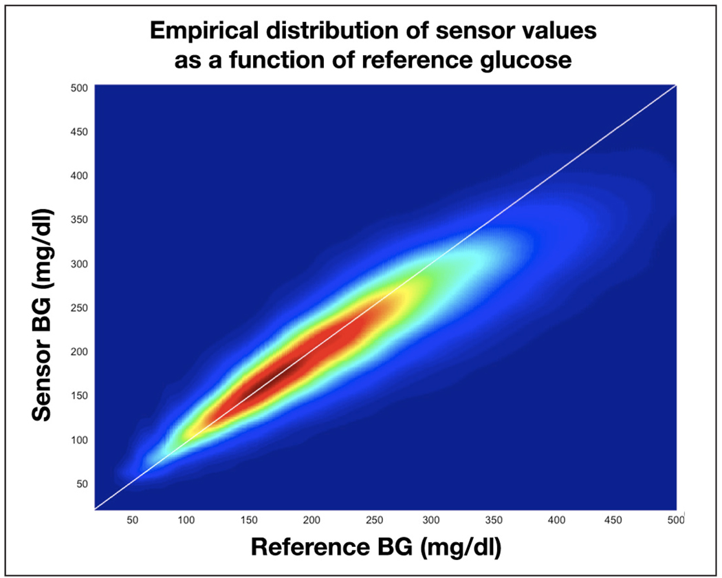
Using data set 1 we studied the sensor response at different reference glucose levels by estimating the probability distribution of the reference/sensor pairs (recalibrated but not synchronized). The distribution is presented in Figure 1, where blue depicts a very low and red a very high probability of occurrence. We observed that sensors tend to read low at high reference values (the reference/sensor pair tends to fall below the diagonal when the reference is above 200 mg/dl) and high at low reference levels (the reference/sensor pair tends to fall above the diagonal when the reference is below 110 mg/dl). Also, the spread of reference/sensor pairs is positively correlated with the reference level: the distribution is flatter at high glucose levels compared to low glucose levels.

Figure 1.

Distribution of the reference glucose/sensor readings for data set 1.

Effect of Rate of Change on Sensor Error and Delay Estimation

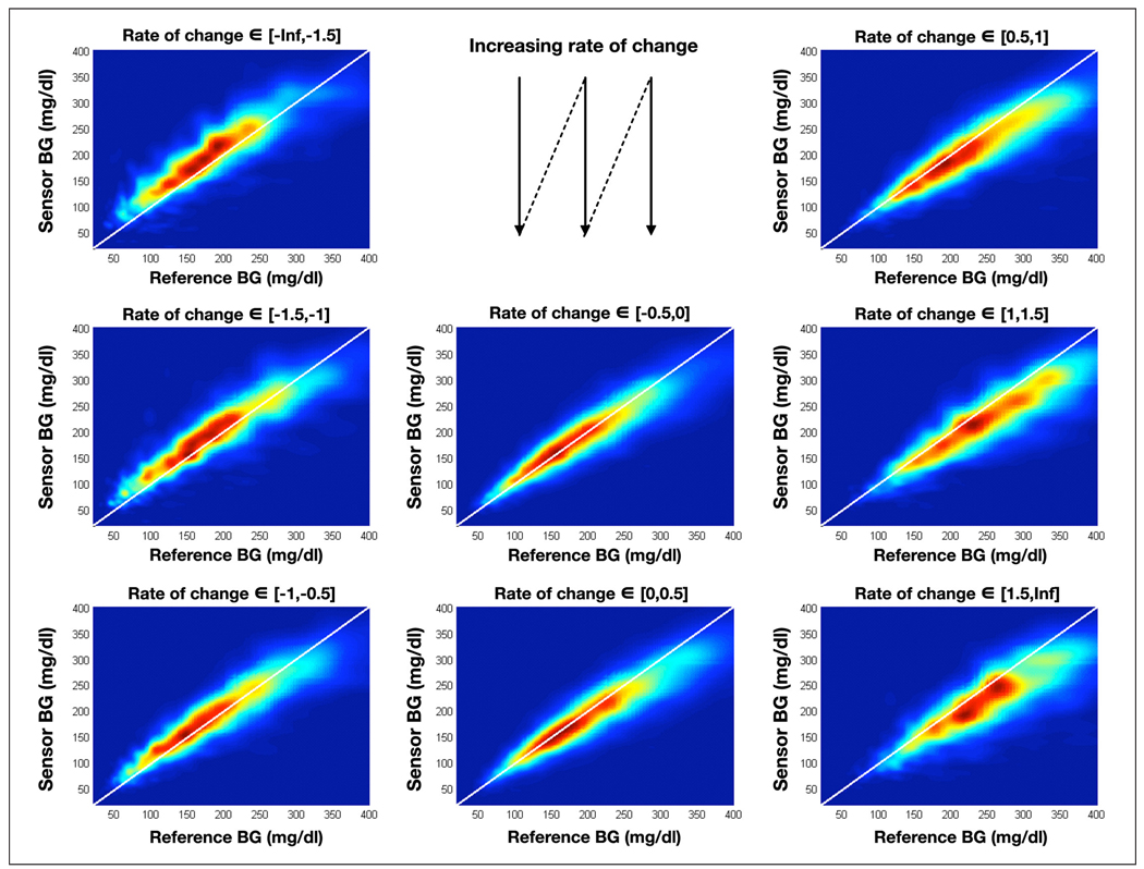
As presented in the introduction, it is widely believed that there is a delay between BG and IG. To verify this claim, we applied the same technique described in the previous section but we clustered the reference/sensor pairs by glucose rate of change: 8 bins of rate of change were selected, the number of pairs in each bin was not constant but was always greater than 1000, the number of pairs per bin was also fairly symmetric around a 0 rate of change, i.e. there were roughly as many pairs between −1.5 and −1 mg/dl/min as between 1 and 1.5 mg/dl/min. This distribution of pairs by rate of change corresponds to the usually accepted distribution of rate of change in the field,²³ therefore indicating an absence of bias. The distributions for each are presented in Figure 2.

Figure 2.

Empirical distribution of the reference/sensor pairs divided in bins based on the rate of change in glucose. BG is expressed in mg/dl.

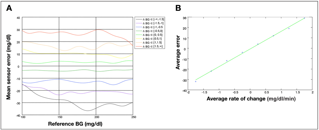
Observing the distributions in Figure 2, particularly the most likely reference/sensor area (red zone in each distribution), we saw that: (i) at a negative rate of change, the sensors tends to read high (red zone above the diagonal); (ii) at a positive rate, the sensors tend to read low (red zone below the diagonal); and (iii) the extent to which the sensor systematically reads high or low is correlated to the amplitude of the rate of change (e.g., the red zone is further above the 45° line in the top left distribution than the bottom left distribution). To verify the last observation, we computed the average reference/sensor discrepancy as a function of the reference glucose for each glucose rate of change bin (j) using the distribution D_j(s,r). The results of this analysis are presented in Figure 3A. We conclude that there exists a correlation between rate of change and average discrepancy, regardless of reference BG levels. Finally, computing the average reference/sensor discrepancy for a specific rate of change across reference values, we compared these averages with the average rate of change in each bin. The results of this analysis are presented in Figure 3B. The average discrepancy is linearly related to the rate of change (R² = 0.995), and the slope of this linear relation (without offset) gives an estimate of the delay, which in this data set is 17 minutes.

Figure 3.

(A) Effect of the glucose rate of change on the mean sensor/reference discrepancy. (B) Estimation of the sensor delay using the average reference/sensor discrepancy at different levels of glucose rate of change.

Characterization of Recalibrated Synchronized Sensor Errors

In this section we study the third component of sensor difference from reference, which remains after recalibration and synchronization of sensor and reference data. We refer to this difference as the sensor error. To study more precisely the sensor error and its time dependency, we used data set 2, which contains YSI glucose measurements taken at 15-minute intervals.

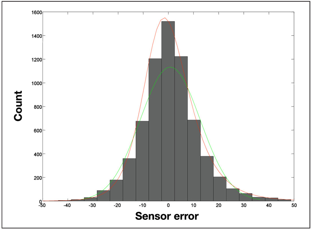
The histogram of the sensor error is presented in Figure 4. The sensor error has a mean of 0.76 mg/dl and a standard deviation of 11 mg/dl, but its skewness and kurtosis show that the distribution of the error is not normal. To estimate its distribution we used the Johnson family and obtain the parameters in Table 1.

Figure 4.

Histogram of sensor error with the fitted normal distribution (green) and the fitted Johnson distribution (red).

Table 1.

Johnson Parameters of the Recalibrated and Synchronized Sensor Error Distribution.

Parameters	Sensor error value
Family type	Unbounded system
λ	15.96
ξ	−5.471
δ	1.6898
γ	−0.5444

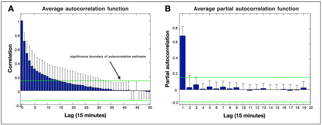
To characterize the time dependency of the sensor error we computed the ACF and PACF of the sensor error as described in the Methods section. Since the reference glucose measures were equally spaced at 15 minutes, the lags are integer multiples of 15 minutes. The results of this analysis are presented in Figure 5. Using a significance bound based on the 95% confidence interval for Gaussian white noise processes; we conclude that sensor noise is highly correlated across time up to several hours. The lag of autocorrelation depends on each sensor (Figure 5A), but, in general, sensor noise is best predicted by a linear combination of the sensor noise 15 minutes earlier and a random white noise term (PACF cutting off after lag 1 in Figure 5B).

Figure 5.

(A) Autocorrelation function of the sensor error with lag intervals of 15 minutes. (B) Partial autocorrelation function of the sensor error with lag interval of 15 minutes.

Modeling of Subcutaneous Sensors

We found that the discrepancy between sensor and reference glucose differ from random noise by having substantial time-lag dependence and other non–independent identically distributed (iid) characteristics (i.e., the error is independent of previous errors and drawn from the same time-independent probability distribution). The components of the discrepancy are therefore modeled as follows:

1. Blood-to-interstitium glucose transport described by Equation (6). Here IG is the interstitial and BG is the plasma glucose concentration; τ represents the time lag between the two fluids.

2. Sensor lag: the time of glucose transport from the interstitium to the sensor needle in Equation (6). Considering that these are two sequential first order diffusion models, we modeled them with one diffusion equation where the time lag is the resultant single diffusion process representing both the physiological lag and the sensor lag. Empirical estimation gives a time lag of 5 minutes (which produces a delay of approximately 15 minutes).

   $$\{\begin{array}{l}\frac{\partial \mathit{IG}}{\partial t}=\frac{1}{\tau }(\mathit{IG}-\mathit{BG})\\ \frac{\partial G}{\partial t}=\frac{1}{{\tau }_N}(G-\mathit{IG})\end{array}$$ (6)
3. The noise of the sensor is non-white, non-Gaussian. We therefore used an autoregressive moving average (ARMA) process for its modeling. Based on the analysis of the empirical partial autocorrelation function in data set 2, we restricted this model to a simple autoregressive model of order 1, [see Equation (7)]. This is due to the apparent non-significance of any PACF coefficient for lags greater than 1. The sensor noise is ε_n′, which is driven by the normally distributed time series e_n. The parameters ξ, λ, δ, and γ are the Johnson system (unbounded system) parameters corresponding to the empirical noise distributions, as shown in Table 1. Validation of these model choices and fits is presented in Figure 6.

   $$\begin{array}{l}\{\begin{array}{l}{e}_1={\upsilon }_1\\ e_n={0.7}^{*}(e_{n-1}+{\upsilon }_n)\end{array}\\ {\upsilon }_n\sim \mathrm{\Phi }(0,1)\text{iid}\\ {\epsilon }_n=\mathrm{\xi }+\lambda \text{sinh}\left(\frac{e_n-\gamma }{\mathrm{\delta }}\right)\end{array}$$ (7)

Figure 6.

Simulated sensor trace and validation against empirical distribution and PACF.

These equations were included in a glucose homeostasis simulator,²² implemented in Matlab Simulink®. An example is presented in Figure 6, along with validation of the modeling by comparing the sensor error distributions (empirical and from simulation), as well as the partial autocorrelation functions. No difference between empirical and simulated characteristics was apparent. Moreover, a χ² test showed that no significant difference exists between the observed and the simulated distribution of sensor errors and the distribution of errors of the FreeStyle Navigator (p > .46).

Conclusions

In this paper, we presented a sequence of analytical techniques beginning with the decomposition of CGM sensor errors into errors due to calibration, blood-to-interstitial glucose transport, and additive noise, leading to computer simulation and building of an in silico sensor based on diffusion and time series modeling. We should emphasize that the term sensor “error”, although well accepted, may not be entirely accurate because part of the “error” is due to physiological processes that result in natural deviations of sensor readings from reference BG levels.

Regardless of terminology, sensor deviations from reference BG levels are generally explained by the specifics of CGM technology—the measurement of glucose takes place in the interstitial compartment, which is associated with, but different from blood. However, CGMs are calibrated against BG, and their accuracy is assessed by comparing IG readings to reference BG. This alone creates two sources of CGM errors, or deviations: calibration and the BG-to-IG gradient.

During analysis, the errors due to calibration can be separated by recalibrating the sensor trace using all available reference BG readings, which is the first step of sensor accuracy analysis. The differences between IG and BG are most evident during rapid BG excursions: sensor errors tend to be negative (high CGM readings) when the BG rate of change is negative and positive (low CGM readings) when the BG rate of change is positive, which is potentially explained by the time lag between the two compartments. This second component of sensor error due to the BG-to-IG gradient can be evaluated by a diffusion model—a commonly accepted technique explaining the possible physiological time lag between blood and IG concentration.^14–16 After recalibration and accounting for the BG-to-IG gradient, the residual sensor noise appears to be non-white (non-Gaussian) and the consecutive sensor errors are highly interdependent. Thus, the presented analysis of residual (after calibration and diffusion) sensor errors is based on time-series approaches using ARMA noise to account for the interdependence between consecutive sensor errors. As an example, we presented the autocorrelation and the distribution of the errors of the FreeStyle Navigator.

Based on the presented sequence of mathematical models, the computer simulation of sensor errors becomes possible. Such an in silico sensor includes both generic deviations due to physiology and sensor-specific errors due to particular sensor engineering. The generic deviations can be approximated reasonably well by a diffusion model. The sensor-specific errors appear to be generally limited to the order of the ARMA model and the shape of the sensor error distribution. Thus, both types of errors can be described by a few model parameters and included in a simulation. A specific type of error is omitted by this methodology: high frequency errors (period of 1 to 15 minutes) cannot be modeled with our techniques. At this time no data are available to extract the characteristic of the error at that fine a sample frequency (we would need reference values every minute in a large data set). Nonetheless, the development of a simulated sensor becomes feasible and became a component of the larger metabolic system simulator developed at the University of Virginia and the University of Padova. This simulator was accepted by the Food and Drug Administration for pre-clinical testing of closed-loop glucose control strategies. Such in silico testing is now employed by the Juvenile Diabetes Research Foundation Artificial Pancreas Consortium, provides insights on the effectiveness of control algorithms during realistic conditions, and allows the direct transition from in silico testing to clinical trials.

Abbreviations

(ACF)

autocorrelation function

(ARMA)

autoregressive moving average

(BG)

blood glucose

(CGM)

continuous glucose monitor

(iid)

independent identically distributed

(IG)

interstitial glucose

(PACF)

partial autocorrelation function

(SMBG)

self-monitored blood glucose

References

- 1.Klonoff DC. Continuous glucose monitoring: Roadmap for 21st century diabetes therapy. Diabetes Care. 2005;28(5):1231–1239. doi: 10.2337/diacare.28.5.1231. [DOI] [PubMed] [Google Scholar]
- 2.Garg K, Zisser H, Schwartz S, Bailey T, Kaplan R, Ellis S, Jovanovic L. Improvement in glycemic excursions with a transcutaneous, real-time continuous glucose sensor. Diabetes Care. 2006;29(1):44–50. doi: 10.2337/diacare.29.01.06.dc05-1686. [DOI] [PubMed] [Google Scholar]
- 3.Deiss D, Bolinder J, Riveline J, Battelino T, Bosi E, Tubiana-Rufi N, Kerr D, Phillip M. Improved Glycemic Control in Poorly Controlled Patients with Type 1 Diabetes Using Real-Time Continuous Glucose Monitoring. Diabetes Care. 2006;29(12):2730–2732. doi: 10.2337/dc06-1134. [DOI] [PubMed] [Google Scholar]
- 4.Kovatchev B, Clarke W. Continuous glucose monitoring (CGM) reduces risks for hypo- and hyperglycemia and glucose variability in diabetes. Diabetes. 2007;56 Suppl 1:A23. [Google Scholar]
- 5.Gerritsen M, Jansen JA, Lutterman JA. Performance of subcutaneously implanted glucose sensors for continuous monitoring. Neth J Med. 1999;54(4):167–179. doi: 10.1016/s0300-2977(99)00006-6. [DOI] [PubMed] [Google Scholar]
- 6.Gross TM, Bode BW, Einhorn D, Kayne DM, Reed JH, White NH, Mastrototaro JJ. Performance evaluation of the MiniMed continuous glucose monitoring system during patient home use. Diabetes Technol Ther. 2000;2(1):49–56. doi: 10.1089/152091500316737. [DOI] [PubMed] [Google Scholar]
- 7.Cheyne EH, Cavan DA, Kerr D. Performance of a continuous glucose monitoring system during controlled hypoglycaemia in healthy volunteers. Diabetes Technol Ther. 2002;4(5):607–613. doi: 10.1089/152091502320798222. [DOI] [PubMed] [Google Scholar]
- 8.Kovatchev BP, Gonder-Frederick LA, Cox DJ, Clarke WL. Evaluating the accuracy of continuous glucose-monitoring sensors: continuous glucose error-grid analysis illustrated by TheraSense FreeStyle Navigator data. Diabetes Care. 2004;27(8):1922–1928. doi: 10.2337/diacare.27.8.1922. [DOI] [PubMed] [Google Scholar]
- 9.Clarke WL, Anderson S, Farhy L, Breton M, Gonder-Frederick L, Cox D, Kovatchev B. Evaluating the clinical accuracy of two continuous glucose sensors using continuous glucose-error grid analysis. Diabetes Care. 2005;28(10):2412–2417. doi: 10.2337/diacare.28.10.2412. [DOI] [PubMed] [Google Scholar]
- 10.Clarke WL, Kovatchev BP. Continuous glucose sensors—continuing questions about clinical accuracy. J Diabetes Sci Technol. 2007;1:164–170. doi: 10.1177/193229680700100510. [DOI] [PMC free article] [PubMed] [Google Scholar]
- 11.Zisser H, Shwartz S, Rather R, Wise J, Bailey T. Accuracy of a seven-day continuous glucose sensor compared to YSI blood glucose values. Proceedings of the 27th Workshop of the Study Group on Artificial Insulin Delivery, Pancreas and Islet Transplantation (AIDPIT) of the European Association for the Study of Diabetes (EASD) and 2nd European Diabetes Technology and Transplantation Meeting (EuDTT); 2008 Jan 27–29; Innsbruck-Igls, Austria. p. 90. AIDPIT; Abstract S03, Available from http://www.aidpit.org. [Google Scholar]
- 12.Facchinetti A, Sparacino G, Cobelli C. Reconstruction of glucose in plasma from interstitial fluid continuous glucose monitoring data: role of sensor calibration. J Diabetes Sci Technol. 2007;1(5):617–623. doi: 10.1177/193229680700100504. [DOI] [PMC free article] [PubMed] [Google Scholar]
- 13.King C, Anderson SM, Breton M, Clarke WL, Kovatchev BP. Modeling of calibration effectiveness and blood-to-interstitial glucose dynamics as potential confounders of the accuracy of continuous glucose sensors during hyperinsulinemic clamp. J Diabetes Sci Technol. 2007;1(3):317–322. doi: 10.1901/jaba.2007.1-317. [DOI] [PMC free article] [PubMed] [Google Scholar]
- 14.Kulcu E, Tamada JA, Reach G, Potts RO, Lesho MJ. Physiological differences between interstitial glucose and blood glucose measured in human subjects. Diabetes Care. 2003;26(8):2405–2409. doi: 10.2337/diacare.26.8.2405. [DOI] [PubMed] [Google Scholar]
- 15.Boyne MS, Silver DM, Kaplan J, Saudek CD. Timing of changes in interstitial and venous blood glucose measured with a continuous subcutaneous glucose sensor. Diabetes. 2003;52(11):2790–2794. doi: 10.2337/diabetes.52.11.2790. [DOI] [PubMed] [Google Scholar]
- 16.Steil GM, Rebrin K, Hariri F, Jinagonda S, Tadros S, Darwin C, Saad MF. Interstitial fluid glucose dynamics during insulin induced hypoglycaemia. Diabetologia. 2005;48(9):1833–1840. doi: 10.1007/s00125-005-1852-x. [DOI] [PubMed] [Google Scholar]
- 17.Hastie T, Tibshirani R, Friedman J. Springer Series in Statistics. 1st ed. New York: Springer; 2001. The elements of statistical learning: Data mining, inference, and prediction. [Google Scholar]
- 18.Johnson NL. Systems of frequency curves generated by methods of translation. Biometrika. 1949;36(1):149–176. [PubMed] [Google Scholar]
- 19.Breton MD, DeVore MD, Brown DE. A tool for systematically comparing the power of tests for normality. J Statistical Computation & Simulation. 2007 Jul; Available from http://www.informaworld.com/smpp/content~content=a780645596?words=breton%7cdevore&hash=3456547477.
- 20.Durbin J. The fitting of time-series models. Rev. Inst. Int. Stat. 1960;28(3):233–244. [Google Scholar]
- 21.Dalla Man C, Raimondo DM, Rizza RA, Cobelli C GIM. Simulation software of meal glucose—insulin model. J Diabetes Sci Technol. 2007;1(3):323–330. doi: 10.1177/193229680700100303. [DOI] [PMC free article] [PubMed] [Google Scholar]
- 22.Brockwell PJ, Davis RA. Springer Series in Statistics. 2nd ed. London: Springer; 1998. Time series: theory and methods. [Google Scholar]
- 23.Kovatchev BP, Clarke WL, Breton M, Brayman K, McCall A. Quantifying temporal glucose variability in diabetes via continuous glucose monitoring. mathematical methods and clinical application. Diabetes Technol Ther. 2005;7(6):849–862. doi: 10.1089/dia.2005.7.849. [DOI] [PubMed] [Google Scholar]