Reduced anatomical clutter in digital breast tomosynthesis with statistical iterative reconstruction

Abstract

Purpose:

Digital breast tomosynthesis (DBT) has been shown to somewhat alleviate the breast tissue overlapping issues of two-dimensional (2D) mammography. However, the improvement in current DBT systems over mammography is still limited. Statistical image reconstruction (SIR) methods have the potential to reduce through-plane artifacts in DBT, and thus may be used to further reduce anatomical clutter. The purpose of this work was to study the impact of SIR on anatomical clutter in the reconstructed DBT image volumes.

Methods:

An SIR with a slice-wise total variation (TV) regularizer was implemented to reconstruct DBT images which were compared with the clinical reconstruction method (filtered backprojection). The artifact spread function (ASF) was measured to quantify the reduction of the through-plane artifacts level in phantom studies and microcalcifications in clinical cases. The anatomical clutter was quantified by the anatomical noise power spectrum with a power law fitting model: NPS_a(f) = αf ^–β. The β values were measured from the reconstructed image slices when the two reconstruction methods were applied to a cohort of clinical breast exams (N = 101) acquired using Hologic Selenia Dimensions DBT systems.

Results:

The full width half maximum (FWHM) of the measured ASF was reduced from 8.7 ± 0.1 mm for clinical reconstruction to 6.5 ± 0.1 mm for SIR which yields a 25% reduction in FWHM in phantom studies and the same amount of ASF reduction was also found in clinical measurements from microcalcifications. The measured β values for the two reconstruction methods were 3.17 ± 0.36 and 2.14 ± 0.39 for the clinical reconstruction method and the SIR method, respectively. This difference was statistically significant (P ≪ 0.001). The dependence of β on slice location using either method was negligible.

Conclusions:

Statistical image reconstruction enabled a significant reduction of both the through-plane artifacts level and anatomical clutter in the DBT reconstructions. The β value was found to be β≈2.14 with the SIR method. This value stays in the middle between the β≈1.8 for cone beam CT and β≈3.2 for mammography. In contrast, the measured β value in the clinical reconstructions (β≈3.17) remains close to that of mammography.

1. INTRODUCTION

Digital breast tomosynthesis (DBT) is an emerging breast imaging modality that builds on existing equipment and techniques used in mammography by incorporating three dimensional (3D) information.¹ Since becoming clinically available in the United States² in 2011, the clinical use of DBT has rapidly expanded. Some of the major benefits of DBT are that it offers in-plane spatial resolution comparable to that of mammography while simultaneously alleviating two major problems inherent to two-dimensional (2D) imaging modalities: (a) overlaying structures obscuring important pathology (false negatives leading to decreased sensitivity) and (b) overlaying structures simulating pathology when none is present (false positives leading to decreased specificity).^3–6 In order to generate this additional spatial information, a series of cone-beam projection images are acquired about the compressed breast over a limited angular span (from 15° to 50° in current clinical systems).⁷ These projection data are then reconstructed in a pseudo-tomographic manner to generate a 3D image volume.

The primary objective in breast imaging (in breast cancer screening in particular) is to determine whether or not a malignancy is present. However, the normal anatomical background in images may significantly confound this task. The impact of the anatomical clutter on detection performance has been quantified using several techniques^8–12 including a spatial frequency-dependent power spectrum, viz., the anatomical background noise power spectrum.^10–12 In the presence of structural anatomical clutter, the overall detectability for a specific imaging task is jointly impacted by a generalized noise power spectrum that consists of two major components: quantum noise and background anatomical clutter.^10–12 The quantum noise depends on a variety of physical factors of the imaging system (such as the quantum detection efficiency of the detector), image acquisition parameters (such as the overall radiation exposure level and tube potential), and the breast itself (such as density, compressed thickness, etc.). On the other hand, the variability in the normal breast parenchymal structure results in an inherent anatomical clutter of the breast. The final apparent anatomical clutter or noise will depend on this inherent anatomical clutter as well as imaging conditions, imaging geometry (compression, CC vs MLO planar view, etc.), modality, reconstruction technique, and image postprocessing.¹³

It is well understood that the level of anatomical clutter has a strong impact on lesion detection performance.^12,14–17 Therefore, quantitative assessment and prediction of diagnostic performance for mammography should take into consideration not only imaging system/acquisition parameters but also the anatomical clutter. As an example, the concept of a generalized NPS including the anatomical clutter has been developed and incorporated into the model observer framework.¹⁸ With this framework, a quantitative understanding of anatomical clutter for a given imaging method may be used to help predict the lesion detection performance for that method.

The anatomical clutter can be quantified using the concept of power spectrum of anatomical background noise that was empirically modeled as¹²:

$${\text{NPS}}_{\text{a}}(f)\approx \alpha f^{-\beta }$$ (1)

where f is the spatial frequency, and α and β are two parameters determined by fitting the measured and radially averaged NPS_a(f) to the model given in Eq. (1). The parameter β has been measured for a variety of breast imaging modalities, including mammography, digital breast tomosynthesis (DBT)¹⁹, and dedicated breast cone-beam CT (BCT).^13,16,20 For each modality, a range of published β values may be found. Not only does β depend on the imaging modality but it also varies with the x-ray beam energy,¹³ breast density,¹⁷ reconstructed tomographic slice thickness,^16,20 and even the imaging plane (e.g., CC vs MLO for mammography and DBT).¹⁶

One way to compare β values across modalities is to use the same patient cohort and measure β values for that cohort using different imaging techniques. In one crossmodality study,¹⁶ the β value was measured in a patient cohort for mammography, DBT, and dedicated breast CT, finding values of β = 3.235 ± 0.090, β = 3.080 ± 0.032, and β = 1.790 ± 0.042 for mammography, DBT, and dedicated breast CT, respectively. These results demonstrated that for the clinical systems tested, moving from mammography to DBT, somewhat surprisingly, only results in a minimal reduction in anatomical clutter. This result can be understood in large part as a result of being limited by through-plane artifacts from the adjacent slices in DBT reconstructions. However, the measured β values are a result of specific DBT imaging system with specific tube, detector, angular span of the acquired cone beam projection angles, and image reconstruction method. Even for a given DBT imaging system, when different angular spans of the acquisition view angles and different image reconstruction methods are used to reconstruct DBT images, the β values may vary. Even if the angular span of the acquisition view angles is fixed, as it is for most currently available clinical DBT imaging systems, different image reconstruction methods may result in different levels of through-plane artifacts and thus, potentially result in different β values.

Given the argument that a reduction in through-plane artifacts level would lead to a potential reduction in anatomical clutter and previous results from other investigators^21–23 demonstrated that a reduction of through-plane artifacts can be achieved in DBT with some statistical image reconstruction (SIR) methods, one may wonder, if the use of SIR in DBT would result in a more pronounced reduction in β values than β≈3.1 from the current clinical reconstructions? If the answer is yes, then what would be the quantitative β values for a specific SIR? The main purpose of this paper was to address these questions.

2. IMAGE RECONSTRUCTION ALGORITHM

To study the impact of SIR on anatomical clutter, the specific image reconstruction algorithm and numerical implementation details must be first specified. In this section, the SIR algorithm used in this work and the associated reconstruction parameters are presented.

2.A. Algorithm and numerical implementation method

In this paper, a well-known edge-preserving regularizer, that is, the total variation (TV) norm of an digital image is chosen to regularize the iterative image reconstruction. For a two-dimensional (2D) M × N vectorized image slice x, the TV norm is defined as follows:

$$TV(x)=\sum _{i=1}^{MN}\sqrt{{\left(x_{i+1}-x_i\right)}^2+{\left(x_{i+N}-x_i\right)}^2}.$$ (2)

Given a system matrix A to model the forward projection of an image volume and a diagonal matrix Q to model the statistical counts of the measured projection data, the log-processed projection data vector y can be used to reconstruct the image vector x by solving the following convex optimization problem:

$$\widehat{x}=\underset{x}{\text{Arg\hspace{0.17em}Min}}\left[\frac{1}{2}\Vert Ax-y{\Vert }_Q^2+\lambda TV(x)\right],$$ (3)

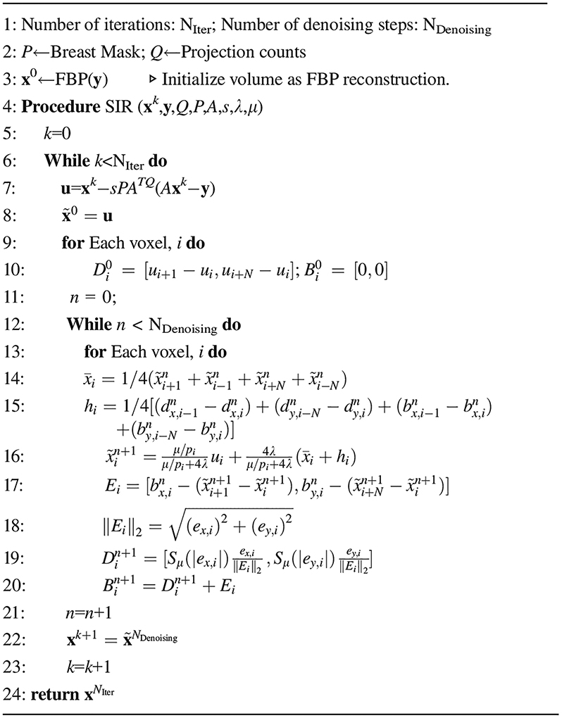
where λ is a parameter controlling regularization strength to model the desired image features such as the noise level and spatial resolution trade-off. Note that the TV norm and its variants have been studied in a constrained optimization framework to address the reconstruction problem with sparse view angles both in x-ray cone-beam CT²⁴ and in DBT.²² In these works, an implementation method known as ASD-POCS^22,24 was developed to iteratively solve the formulated constrained optimization problem. In this paper, rather than solving the constrained optimization problem using ASD-POCS, we start with the more conventional unconstrained optimization problem in Eq. (3). There are many readily available numerical methods to solve the unconstrained optimization problem in Eq. (3). The method used in this paper is the well-known forward-backward proximal splitting method.²⁵ In this method, the solution, $\widehat{x}$, of the convex optimization problem in Eq. (3) is recast as the solution of the following fixed point problem:

$$\widehat{x}={\text{prox}}_{\lambda PTV}\left[\widehat{x}-P{A}^{T}Q(A\widehat{x}-y)\right]$$ (4)

where the positive semi-definite matrix P is a binary mask to define the compact support of the breast image volume and the proximity operator²⁵ prox_λPTV(u) is defined as the solution of the following standard denoising problem:

$${\text{prox}}_{\lambda PTV}(u)=\underset{x}{\text{Arg\hspace{0.17em}Min}}\left[\frac{1}{2}\Vert x-u{\Vert }_{P^{-1}}^2+\lambda TV(x)\right],$$ (5)

The fixed point $\widehat{x}$ in Eq. (4) can be iteratively solved using the following alternating sequences:²⁵

$$u=x^k-sP{A}^{T}Q\left(A{x}^k-y\right),$$ (6)

$$x^{k+1}={\text{prox}}_{\lambda PTV}(u).$$ (7)

Eq. (6) represents a gradient descent update with a statistical penalty matrix Q, a binary mask matrix P, and a step size s.

The denoising problem in Eq. (5) can be iteratively solved using a 2D shrinkage operator $D_i^{n+1}=\left[S_{\mu }\left(\left|e_{x,i}\right|\right)\frac{e_{x,i}}{{\Vert E_i\Vert }_2},S_{\mu }\left(\left|e_{y,i}\right|\right)\frac{e_{y,i}}{{\Vert E_i\Vert }_2}\right]$, where $S_{\mu }(x)=x{\left(1-\frac{\mu }{\left|x\right|}\right)}_{+}$ is the well-known one-dimensional shrinkage operator. This iterative solver is presented in lines 8–22 in the pseudocode of the entire numerical implementation process shown in Algorithm 1. The detailed derivation to obtain this solver using a variable splitting technique²⁶ and the corresponding ADMM was presented in the Appendix of the paper. Additionally, in the numerical implementation, the ordered-subset method²⁷ was used with five subsets, each subset containing three view angles of cone beam projections. Other empirically chosen reconstruction parameters used in this paper to produce images were listed in Table I.

Table I.

Reconstruction parameters.

Parameter	Value
Number of iterations: NIter	50
Number of regularization steps: NDenoising	5
Step size (s)	0.75
λ	12.5
μ	1.25
Q	Generated as described in Eq. (8)
P	Generated as described in Section 2.C.

Algorithm 1:

Pseudocode for the numerical implementation of the SIR used in this work with a 2D TV norm regularizer.

Note: $D^n=\left[d_x^n,d_y^n\right]$, $B^n=\left[b_x^n,b_y^n\right]$, and E=[e_x,e_y]

2.B. Statistical weight matrix Q

As described in Eq. (3), the matrix Q is a diagonal matrix which models the statistical counts of the measured projection data and is used to penalize rays during the reconstruction according to their noise. In other words, a noisy ray with very few photons arriving at the detector is given a smaller weight than a ray where the photon number arriving at the detector is high. Each diagonal element, Q_i, of Q was determined using the measured detector counts and a correction for electronic noise^28,29 as follows:

$$Q_i=\frac{D_i^2}{D_i+{\sigma }_E^2},$$ (8)

where D_i is the measured detector counts at the detector location, i, and ${\sigma }_E^2$ is introduced to account for the detector readout electronics. In this work, the approximate electronic noise variance was estimated by acquiring images with the window of the x-ray tube being blocked with a lead blocker. The variance in the resulting projection images was found to be ${\sigma }_E^2\approx 50$.

2.C. Binary diagonal image mask matrix P for breast volume support

To mitigate truncation artifacts and speed up computation, a 3D breast mask was used to constrain reconstruction.^30,31 This mask approximates the breast support by identifying the breast boundaries in the projection domain, backprojecting the borders, and filling in to the chest wall as shown in Fig. 1. The calculated breast mask was used as the image domain weight, P in Eq. (6). To arrive at Eq. (4), we required that P be positive semidefinite. In our definition here of P as a binary breast mask we meet those criteria since P is diagonal with diagonal elements of either 0 or 1.

Fig. 1.

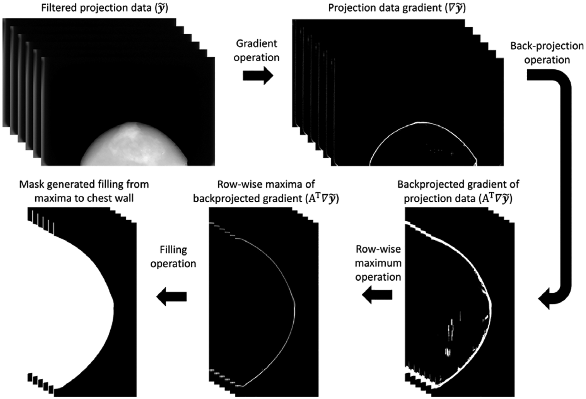
The workflow used to calculate the 3D breast mask volume.

2.D. Forward- and back-projection

In numerical implementation, projection matrices of the imaging system were used to perform both forward- and back-projection.³² Projection matrices provide a calibrated mapping from the image domain to the projection domain. To be more specific, for a given view angle, i, there is a one-to-one correspondence between a location denoted by (u,v) on the detector plane and a voxel location denoted by (x,y,z) in the image volume:

$$\left(\begin{array}{c}u\times s\\ v\times s\\ s\end{array}\right)=B_i\left(\begin{array}{l}x\hfill \\ y\hfill \\ z\hfill \\ 1\hfill \end{array}\right)$$ (9)

where s is a scalar, and B_i is a 3 × 4 matrix, where the subscript i indicates the current projection number. Although B_i itself is not square, for a fixed slice location, z, one can invert the matrix algebraically and use a similar formulation to perform the forward projection as follows:

$$\left(\begin{array}{c}x\times s^{\prime }\\ y\times s^{\prime }\\ s^{\prime }\end{array}\right)=F_i(z)\left(\begin{array}{l}u\hfill \\ v\hfill \\ 1\hfill \end{array}\right)$$ (10)

where s′ is another scalar and F_i(z) is a 3 × 3 z-dependent matrix, where the subscript i indicates the current projection number.

2.E. Computational facilities

The algorithm was coded in Visual C (Microsoft, Inc., Redmond, WA, USA) and CUDA (NVIDIA Corporation, Santa Clara, CA, USA) and executed on a local workstation with dual Xeon E5–2620 CPUs (Intel Corporation, Santa Clara, CA, USA) and 64 GB of RAM and a GTX 1070 GPU (NVIDIA, Santa Clara, CA, USA) GPU with 8 GB of RAM. In the clinical cohort studied for this work, the average total time needed to perform the SIR reconstructions was approximately 70 s.

3. EXPERIMENTAL METHODS AND MATERIALS

In this work, projection data from a patient cohort with 101 patients were retrospectively processed. This cohort included breasts with and without pathology, however, cases with metal, implants, or large calcifications were excluded. The measurements were performed in volumes reconstructed using two methods: the clinical reconstruction (FBP + standard postprocessing) and the SIR method described in Section 2.A. Both the clinical and the SIR-reconstructed volumes had 1 mm slice sampling and a variable in-plane pixel pitch using a projective pixel grid where the pixel pitch is determined by the detector element size and the system magnification for a given slice location as shown in Fig. 2. In this method, voxels further from the detector (closer to the focal spot) are smaller than those closer to the detector. In this work, the voxel size was exactly matched between the clinical reconstruction and the SIR reconstructions.

Fig. 2.

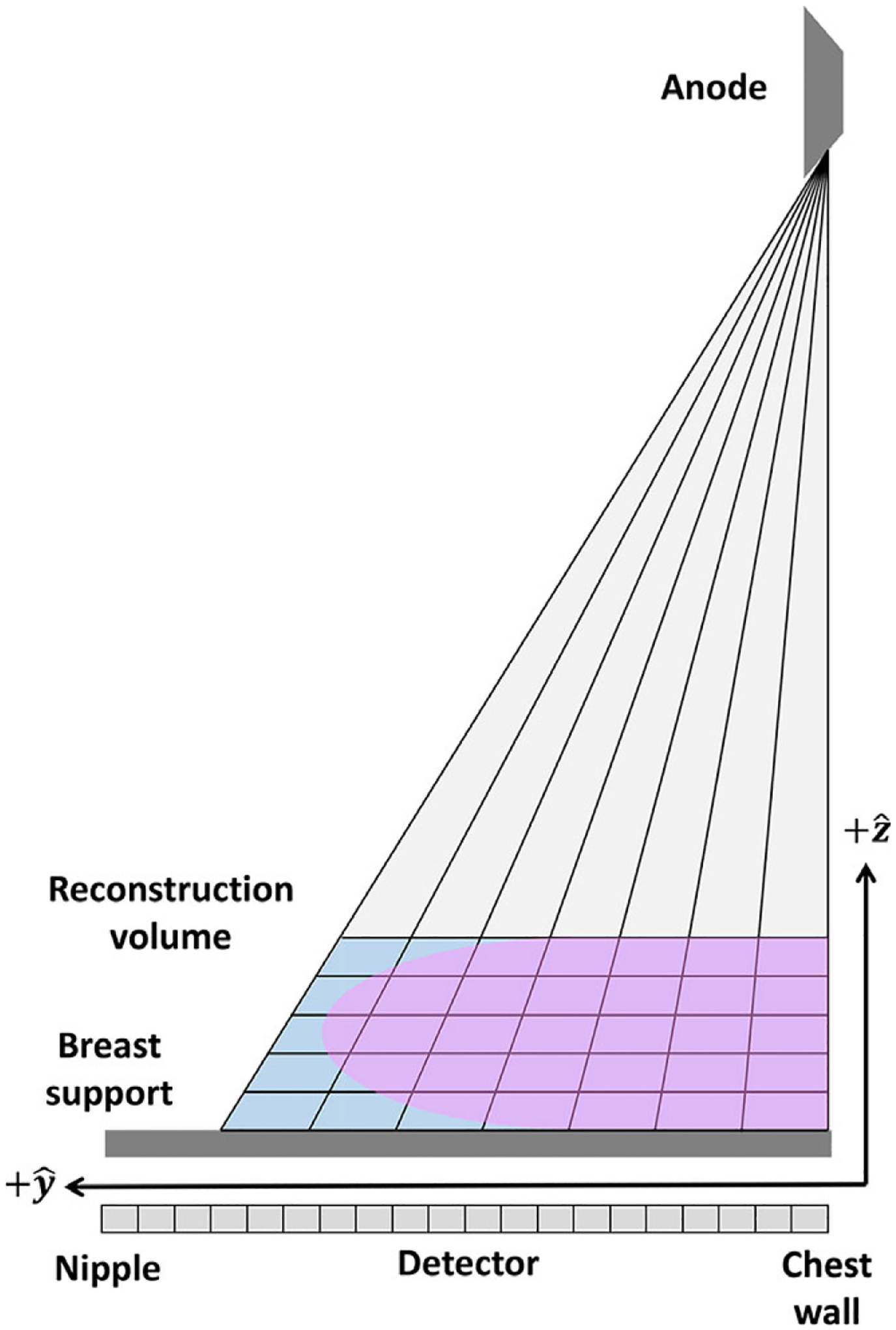
An illustration of the projective pixel grid used in this work.

3.A. Data acquisition

All datasets used in this work were acquired using Hologic Selenia Dimensions (Hologic, Inc. Bedford, MA, USA) DBT imaging systems. A cohort of 101 clinical DBT exams was acquired with IRB approval. This cohort included a mix of both CC and MLO views (63 CC, 38 MLO) with an average breast thickness of 6.7 ± 1.6 cm and average patient age of 55 ± 10 yr. The mean tube potential used was 34 ± 4 kVp, and the average glandular dose (AGD) in the cohort was 2.7 ± 0.9 mGy. Three clinical cases from this cohort were analyzed subjectively and are presented in this work for qualitative image quality assessment for different image reconstruction methods.

3.B. Artifact spread function measurements

To quantify the potential reduction of through-plane artifacts in SIR compared with the clinical reconstruction, the well-known artifact spread function (ASF)^21,33–35 was measured to compare spatial blurring along the slice direction for the two reconstruction methods. To measure the ASF, we placed a 1 mm chrome steel ball (Fastenal Company, Winona, MN, USA) at a height of 25 mm above the breast support in the center of a custom breast-shaped solid water phantom (Gammex, Middleton, WI, USA; see Figs. 3 and 4). The phantom was imaged 25 times using typical imaging parameters (32 kVp, 40 mAs, 1.0 mGy AGD). The ASF was measured according to the following definition:³⁵

$$\text{ASF}(z)=\frac{I_{Max}(z)-{\overline{I}}_{bkg}(z)}{I_{Max}\left(z_0\right)-{\overline{I}}_{bkg}\left(z_0\right)},$$ (11)

where I_Max denotes the maximum intensity value in the region containing the highly attenuating bead, ${\overline{I}}_{bkg}$ denotes the mean value in an adjacent background region, z, denotes the slice position, and z₀ denotes the actual slice location of the highly attenuating bead. The ASF width was quantified using the measured full width half maximum (FWHM) of the ASF in millimeter. To test whether the measured ASF reduction in phantom studies can be generalized to the clinical scenario, we also identified a high-contrast calcification (∅ ≈ 640 μm) in a clinical case (not part of the cohort used to measure β) with a fairly homogeneous background (see Fig. 3) and measured the ASF for that calcification in situ. Note that since this clinical measurement was retrospective, repeated scans were not possible, so a single ASF curve was measured and the result is presented without the error bars.

Fig. 3.

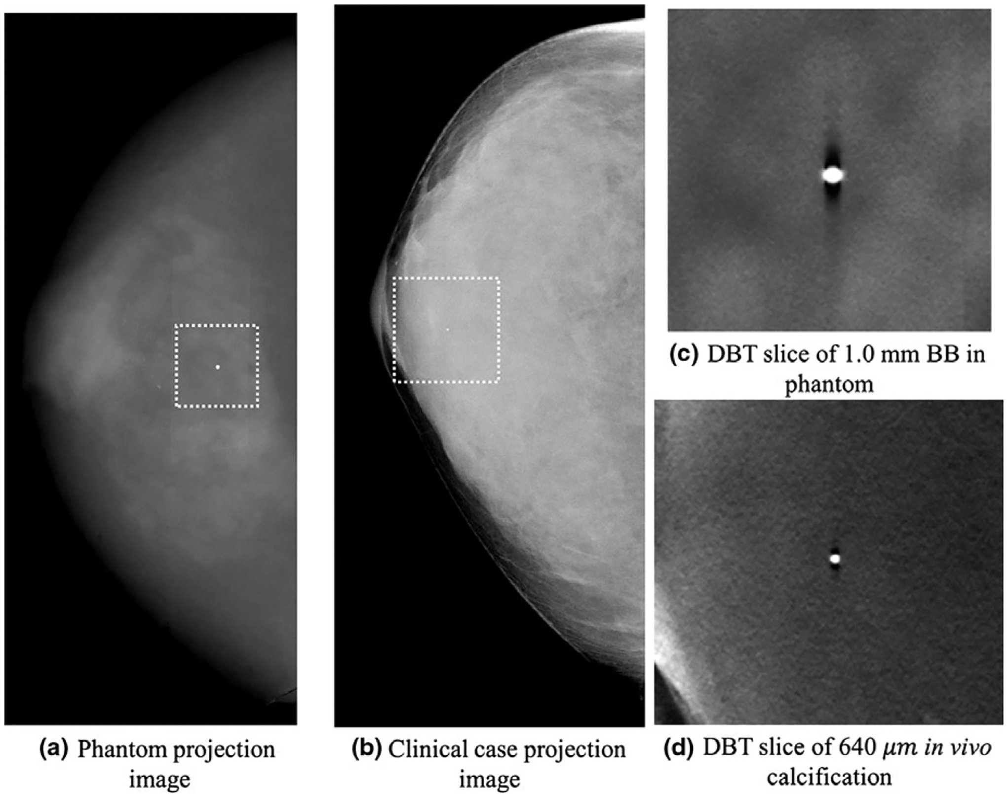
Projection images of the phantom (a) and clinical cases (b) used for the ASF measurements are shown along with the corresponding reconstructions in (c) and (d), respectively.

Fig. 4.

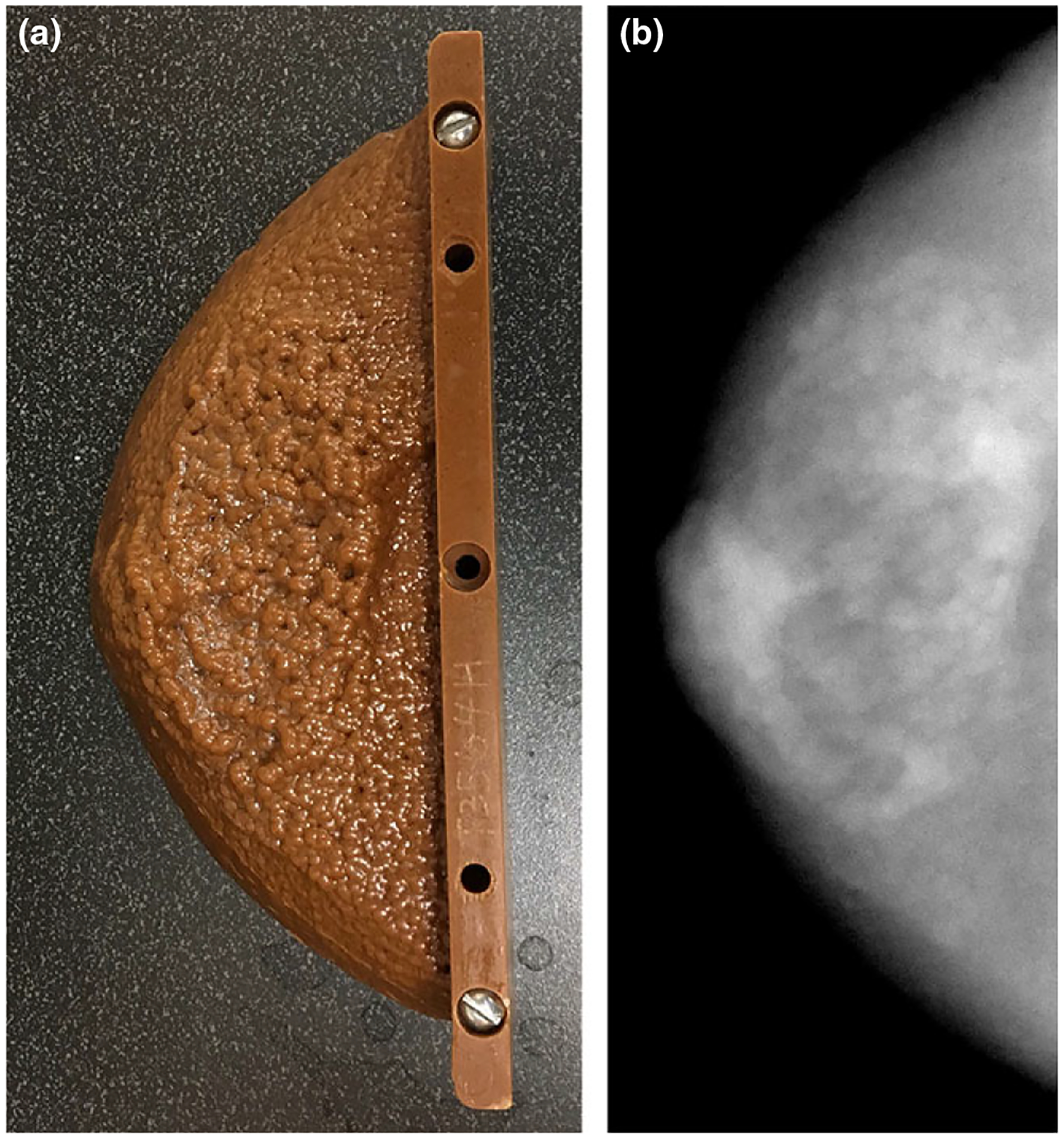
A photograph (a) and radiograph (b) of the custom anthropomorphic phantom used to validate the fitting range used in the measurement of β.

3.C. Anatomical noise power measurement

The anatomical clutter parameter, β, was measured using a previously published method³⁶ in the central 25 slices of each reconstructed volume. In this method, one hundred 256 × 256 ROIs were randomly placed in each reconstructed slice. Each ROI was constrained to fall completely within the breast parenchyma (ROIs straddling the skin line, pectoralis muscle, etc., were rejected). Once a satisfactory ROI was identified, the ROI was windowed using a radial Hanning window to suppress spectral leakage and the power spectrum was calculated. This process was repeated for 100 ROIs per slice to determine an average power spectrum for that slice. A least squares fitting was then performed to determine the parameters α and β. The ROIs were allowed to overlap and were chosen independently for each slice. The selected ROIs were chosen once and then used in both the SIR and clinical reconstruction. It should be pointed out, that since multiple ROIs were chosen from the same subject, there is a possibility of correlations. In this work, any such possible correlations were not taken into account.

Since the anatomical component of the NPS is only dominant in a certain range of frequency values, the power-law fitting of the NPS was performed over a limited frequency range, [f_min,f_max]. This range was carefully chosen by avoiding extremely low frequencies and extremely high frequencies. In previously published work, the recommended frequency ranges vary,^12,15,16,20 with f_min≥0.1mm⁻¹ and f_max≤0.5–1mm⁻¹. In a clinical cohort, there is always interexam variation in both dose (increased/decreased quantum noise contribution) and anatomical clutter. In order to be robust in practice, the frequency range can be selected^15,16 to maximize the coefficient of correlation, r². This range was found by searching all possible frequency ranges (s.t. f_min < f_max) to choose the β value that yielded the best fit with minimal least squared error.

To validate that the selected range indeed corresponded to a frequency range dominated by anatomical clutter, a custom made anthropomorphic phantom (Gammex, Middleton, WI, USA) (see Fig. 4) was imaged using typical imaging parameters (32 kVp, 38 mAs, 1.0 mGy AGD). Using five repeated scans of the phantom, both the quantum only and total noise power spectra were calculated in the slices of the phantom containing simulated anatomical variation and compared for each reconstruction method. The total noise power spectra were calculated directly in the five reconstructed volumes and averaged; the quantum noise power spectrum was calculated by subtracting the ensemble average of the five reconstructions from each reconstruction to generate five noise only volumes.

3.D. Data analysis

The measured β values were compared in several ways. The average β value for each reconstruction method was measured by averaging the measured β values from all the measured slices in each case to calculate a single β value per breast. The average and standard deviation of those measurements (one per case) was calculated.

To determine if any difference in the mean values was significant, a two-sample t test (significance threshold: α = 0.01) was performed in MATLAB (R2017a, The Math-Works, Natick, MA, USA). The null hypothesis was that the means were equal, H₀:μ₁ = μ₂, and thus the alternative hypothesis is a difference in the mean measured value, H₁:μ₁ > μ₂. The measured values for each case were also compared directly in a plot (β_SIRvs.β_Clin), and a linear regression was then performed to determine any correlation between the two reconstruction method.

In addition to comparing the measured β values in the two reconstruction methods, two tests were performed to determine if the two methods treated different breast views or slice positions differently. To compare the two views, the average values were calculated for the MLO and CC views for each reconstruction method. In each case (clinical and SIR reconstructions), the mean values were compared using a two-sample t test as previously described.

Finally, the measured β values were averaged for each slice position (relative to the center of the volume) for each method. This averaging resulted in 25 β measurements per reconstruction method. To determine if β had any dependence on slice position in either reconstruction method, a one-way ANOVA was performed. This ANOVA test compared the measured values at different slice locations with the overall average to determine if the average value at any of the slice locations was significantly different. The null hypothesis was that the mean value at each slice position was equal to the underlying mean across slices, H₀:for alli:μ_i = 〈μ_all〉; the alternative hypothesis was that the mean value at any slice position was different than the underlying mean across all slices H₁:for somei:μ_i > 〈μ_all〉 or μ_i < 〈μ_all〉.

4. RESULTS

4.A. Qualitative comparison of reconstructed images

In the first case (Fig. 5), a cluster of calcifications in a heterogeneously dense breast (BIRADS density: (c); R CC view) from a 40-year-old woman is shown. This cluster of calcifications is well focused and conspicuous in the focal plane in both reconstructions. However, in the clinical reconstruction, the residual signal from the cluster is clearly visible and distracting in the reconstructed slices 10 mm above and below the cluster.

Fig. 5.

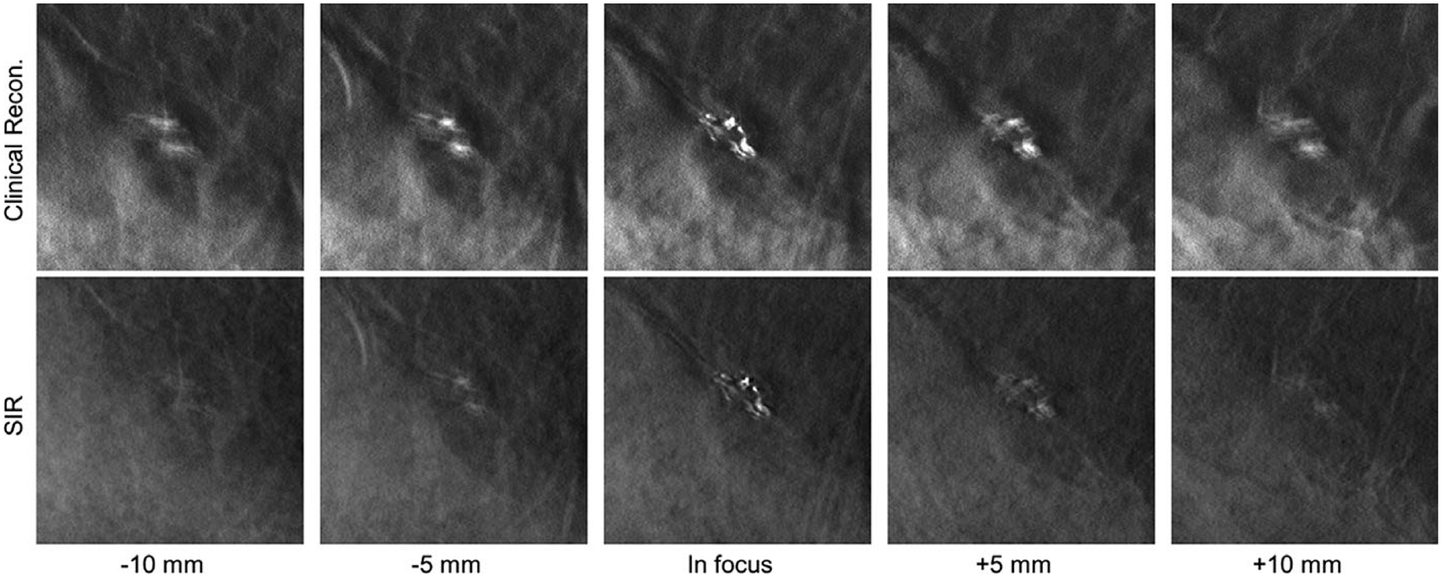
A cluster of calcifications in a clinical DBT exam reconstructed with the clinical reconstruction engine (top) and SIR (bottom) is shown in focus (middle image column) and at locations above (left two image columns) and below (right two image columns) the focal plane in the z direction. All image shown with the same W/L.

In the second case (Fig. 6), a highly calcified dense mass in a fatty breast (BIRADS density: (a); R CC view) of a 69-year-old woman is shown. Subjectively, this is a very interesting pathology with many different high-contrast features present. However, the superposition of the high-contrast features in the clinical reconstruction indicates substantial signal leakage from the nearby image planes and the superposition leads to reduced image sharpness. Both the margins of the mass as well as the calcified structures are difficult to distinguish, and the different layers of the mass are not well separated. In contrast, in the SIR reconstructions, the signal leakage is substantially reduced, and the individual layers of the mass may be clearly differentiated.

Fig. 6.

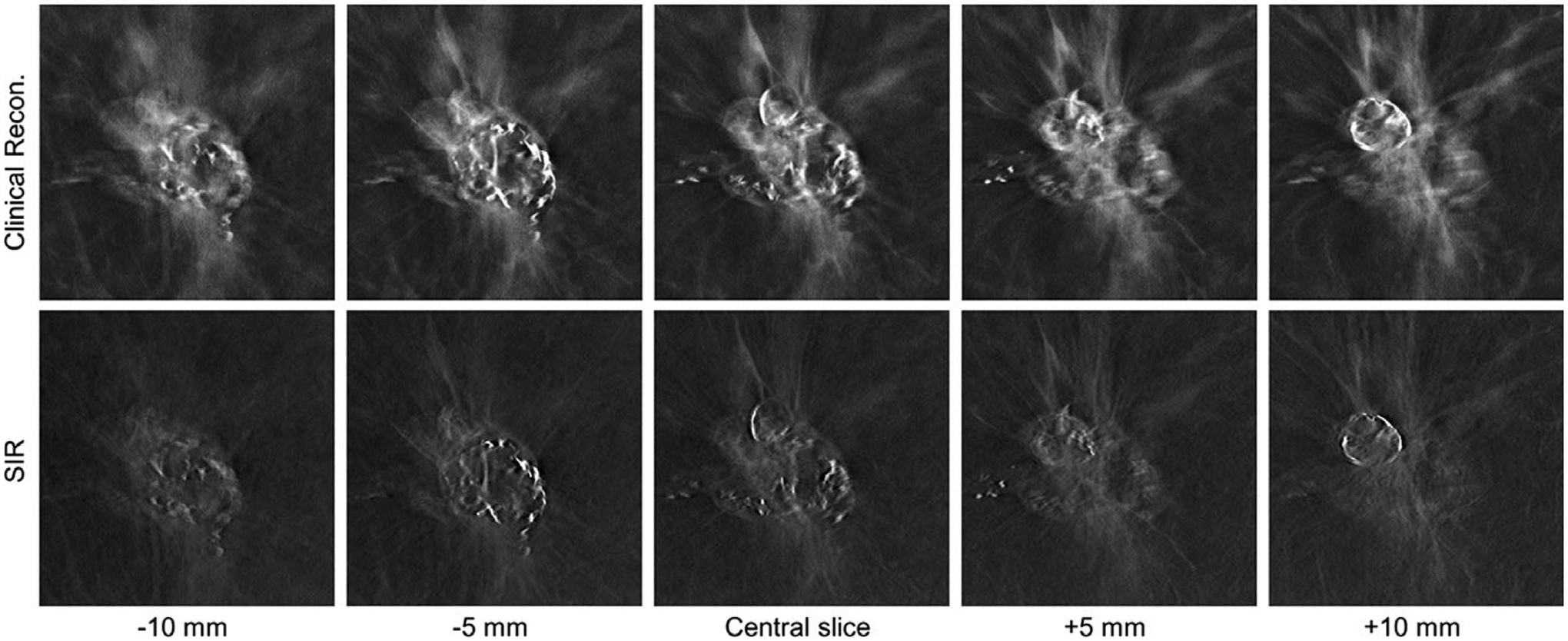
A highly calcified dense mass in a clinical DBT exam reconstructed with the clinical reconstruction engine (top) and SIR (bottom) is shown at different z locations. All images are shown with the same W/L.

In the third case (Fig. 7), a spiculated mass with calcifications in a breast with scattered fibroglandular tissue (BIRADS density: (c); R CC view) of a 67-year-old woman is shown. This case demonstrates some of the issues with FBP at the boundaries of the breast, where the skin line was incorrectly reconstructed, and through-plane blurring obscured the subcutaneous fat.

Fig. 7.

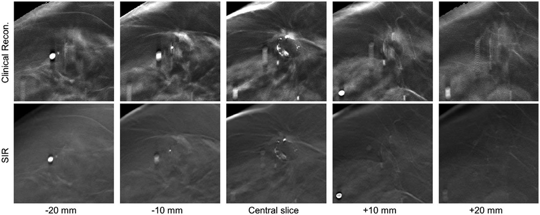
A boundary region in a clinical DBT exam reconstructed with the clinical reconstruction engine (top) and SIR (bottom) is shown at different z locations. All image shown with the same W/L.

4.B. Artifact spread function measurements

The measured ASF curves for the phantom case are shown in Fig. 8 (a). The mean and standard deviations of the FWHM of the ASF measurements in the phantom case were 8.7 ± 0.1 mm for the clinical reconstruction and 6.5 ± 0.1 mm for the SIR method (approximately a 25% improvement). The measured FWHM for the clinical reconstruction is slightly less than the previously published values^34,35 for this system (≈10 mm). The measured ASF curves for the in vivo calcification are shown in Fig. 8(b). The measured FWHM of the ASF was 7.0 and 5.3 mm for the clinical and SIR methods, respectively (again, approximately a 25% improvement).

Fig. 8.

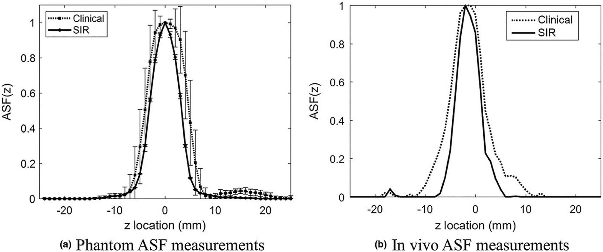
The measured ASF curves for the two reconstruction methods in the phantom (a) and a clinical case (b).

4.C. Anatomical noise power spectrum

4.C.1. Validation of the range of spatial frequencies used in power-law model fitting

For this cohort, the frequency ranges used for the two reconstruction methods are summarized in Table II. To validate that these selected frequency ranges truly correspond to the frequency range dominated by anatomical clutter, the total and quantum only NPS for the anthropomorphic breast phantom are shown in Fig. 9. In the frequency range used to perform the least squares fitting, the total noise power spectrum is strikingly different compared with the quantum only NPS, indicating that contribution to the total NPS in that frequency range is indeed dominated by anatomical clutter. Using these ranges, the correlation was very high in all cases. For the clinical reconstructions, the median r² value was r² = 0.9975, the interquartile range (IQR) was 0.0034, and the range was 0.0219. For the SIR method, the median r² value was r² = 0.9969, the IQR was 0.0039, and the range was 0.0482.

Table II.

The limits of the frequency range used to calculate β for the DBT reconstructions and the corresponding standard deviations for the different reconstruction methods.

	Clinical	SIR
fmin ± σf(mm−1)	0.13 ± 0.03	0.12 ± 0.03
fmax ± σf(mm−1)	0.62 ± 0.12	0.63 ± 0.12

Fig. 9.

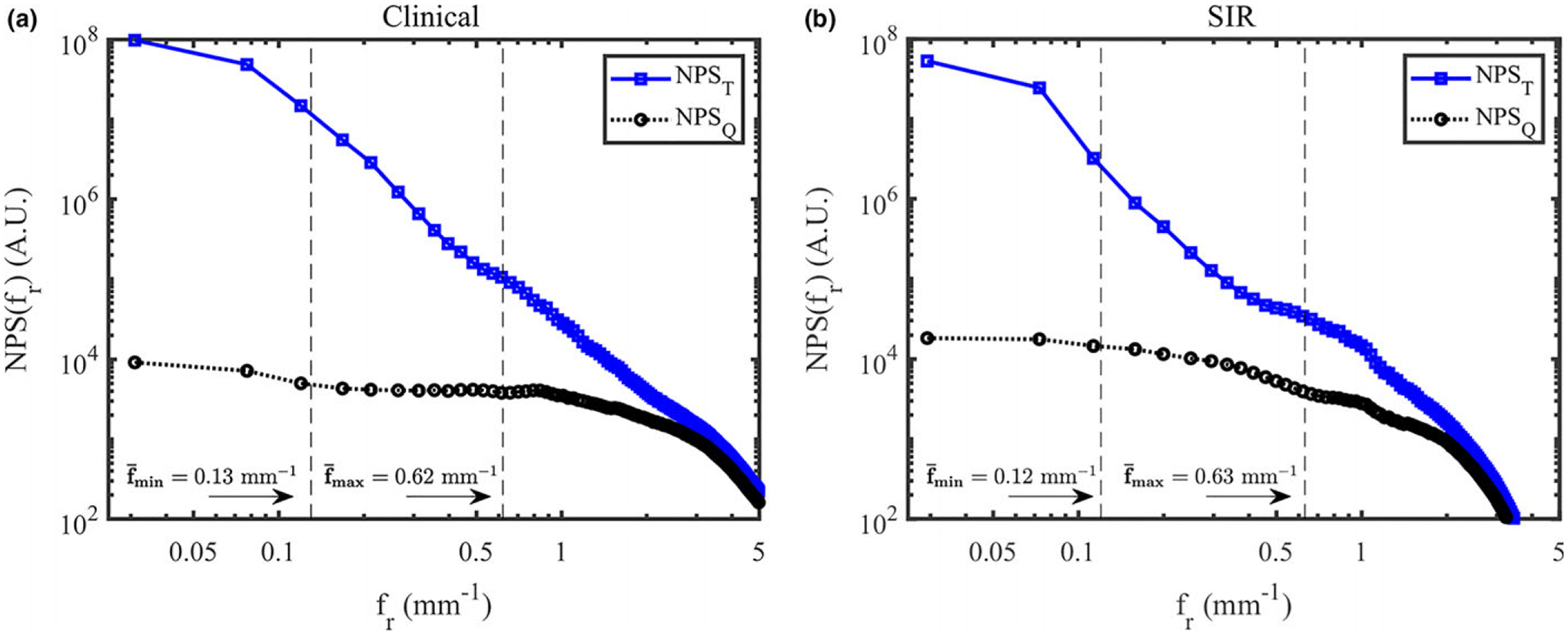
The total and quantum NPS in the anthropomorphic breast phantom using the clinical reconstruction method (a) and SIR (b). The average upper and lower frequency limits used for the power-law fitting in the clinical cohort are shown in this figure.

4.C.2. Dependence on reconstruction method

The average measured NPS along with the corresponding least-squares power-law fits are shown in Fig. 10. The average measured β values and the corresponding standard deviations are shown in Table III. A reduction in β of approximately 1 was seen in the SIR reconstructions compared with the clinical reconstruction. This difference between the mean β values of the two methods was statistically significant (P ≪ 0.001).

Fig. 10.

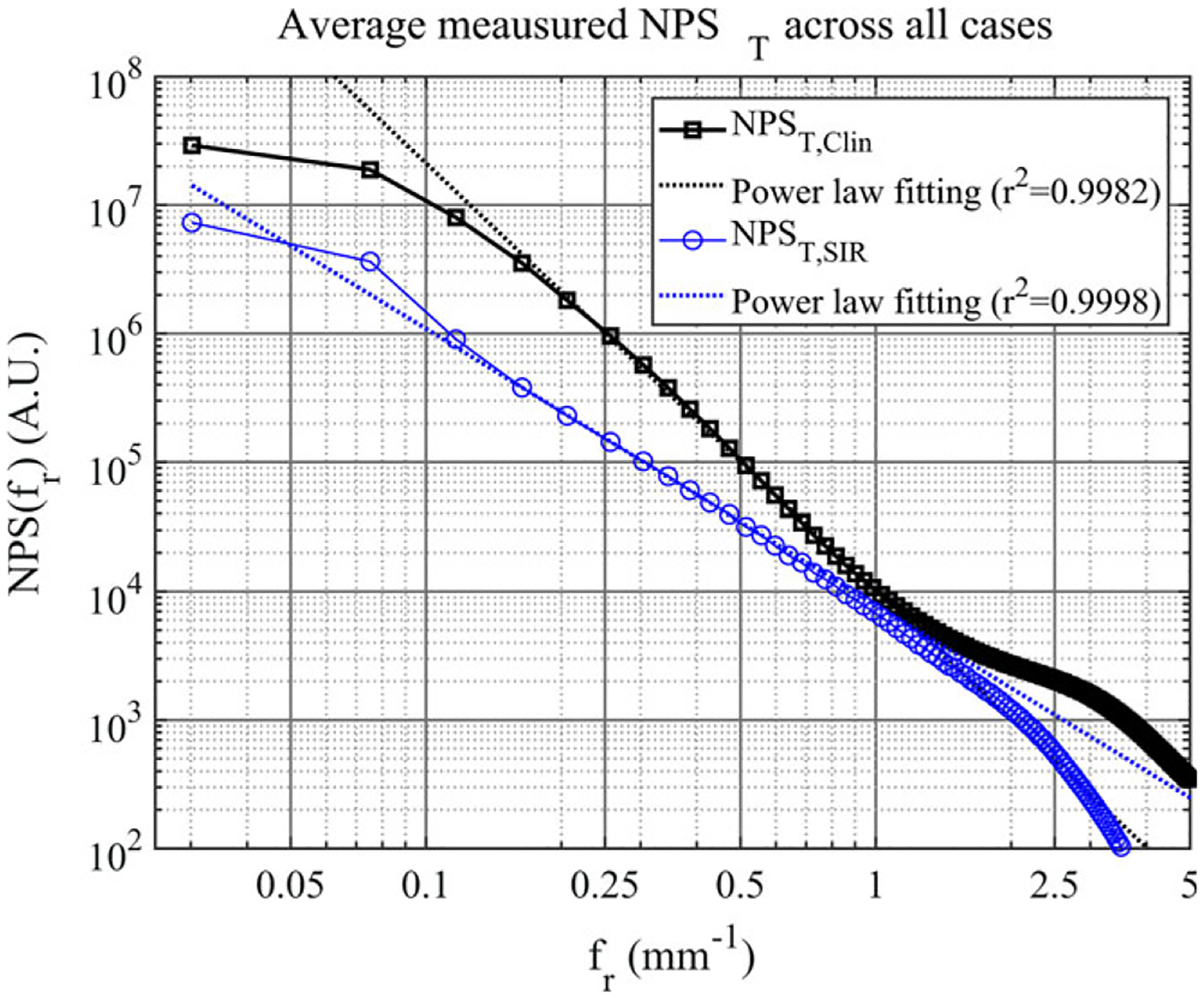
The averaged measured NPS_T for each reconstruction method. The corresponding linear least squares fit is shown as a dashed line for each case.

Table III.

The measured average values of β and the corresponding standard deviations for the different reconstruction methods.

	Clinical	SIR
βmean ± σβ	3.17 ± 0.36	2.14,pm 0.39

As one can observe from Fig. 10, the quantum noise power is much higher for the SIR method at frequencies below0.5mm⁻¹. To understand this phenomenon, it is important to note that, in this work, the regularization parameters were chosen to achieve a similar noise variance (in terms of quantum noise) to the current clinical reconstructions. For the anthropomorphic phantom NPS presented, the approximate noise standard deviation for the quantum noise only was 13 for the clinical reconstructions and 9 for the SIR reconstructions (calculated by integrating the measured quantum NPS to estimate the noise variance). The TV regularization used in this work may preferentially suppress high-frequency noise, and so even though the noise variance is similar in the two reconstructions, the quantum noise power spectrum for the SIR cases does have higher power for low frequencies.

The measured β values using the SIR method are compared with the measured values from the clinical reconstruction in Fig. 11. The least-squares regression of the measured values was plotted as well; the corresponding relationship is provided in the plot legend. The correlation was moderately high (r² = 0.700) and slope of this fit was found to be 0.91, with a negative and nonzero offset of −0.73.

Fig. 11.

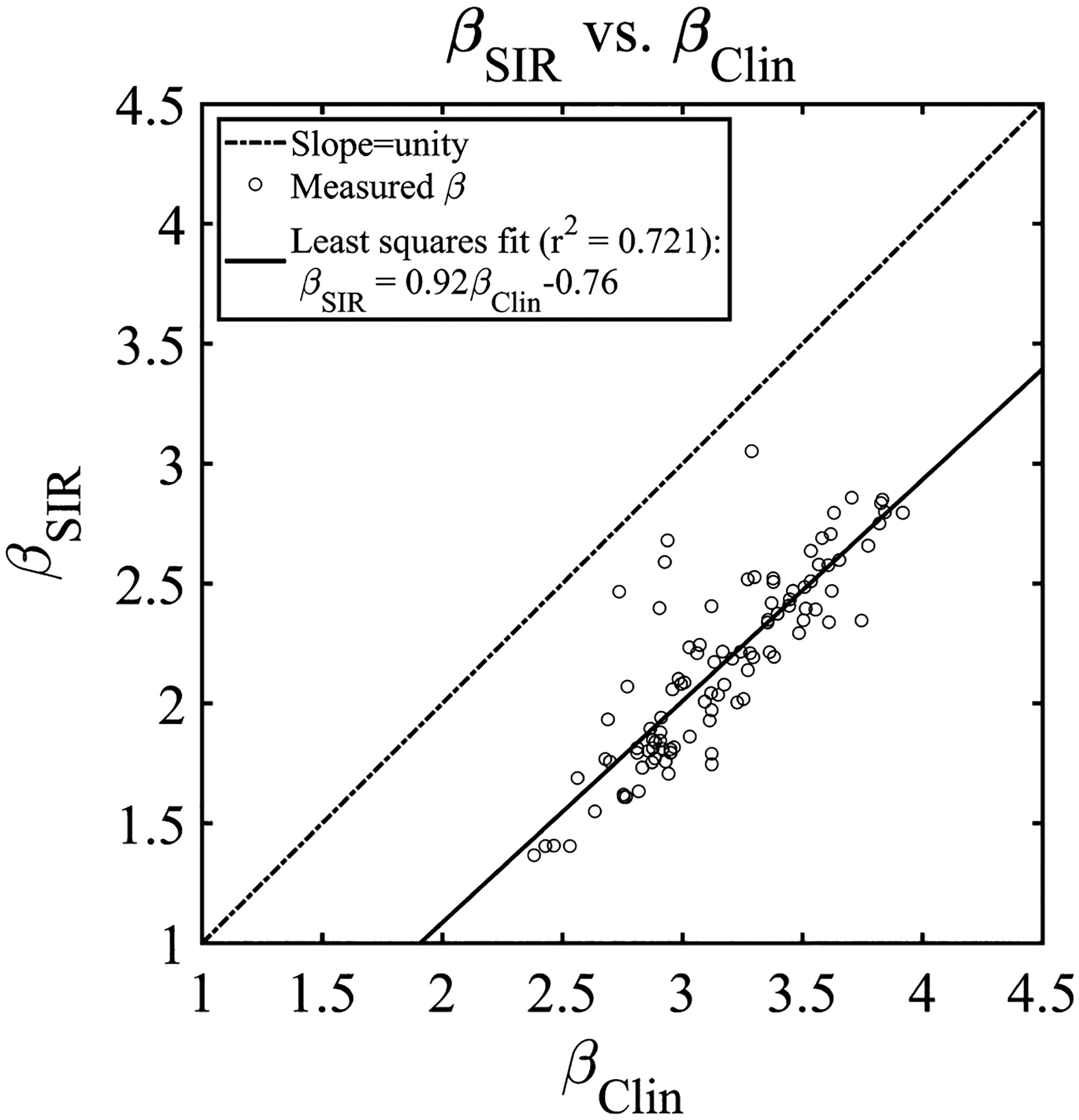
The measured β values for the DOS-SPART DBT reconstructions plotted against the clinical reconstruction. The linear least squares fit is shown in the legend.

4.C.3. Dependence on the acquisition modes: CC vs MLO

The distribution of measured β values in the different views (CC and MLO) is shown in Fig. 12. For each reconstruction method, the difference between the CC and MLO views with each method was not significant (P > 0.01).

Fig. 12.

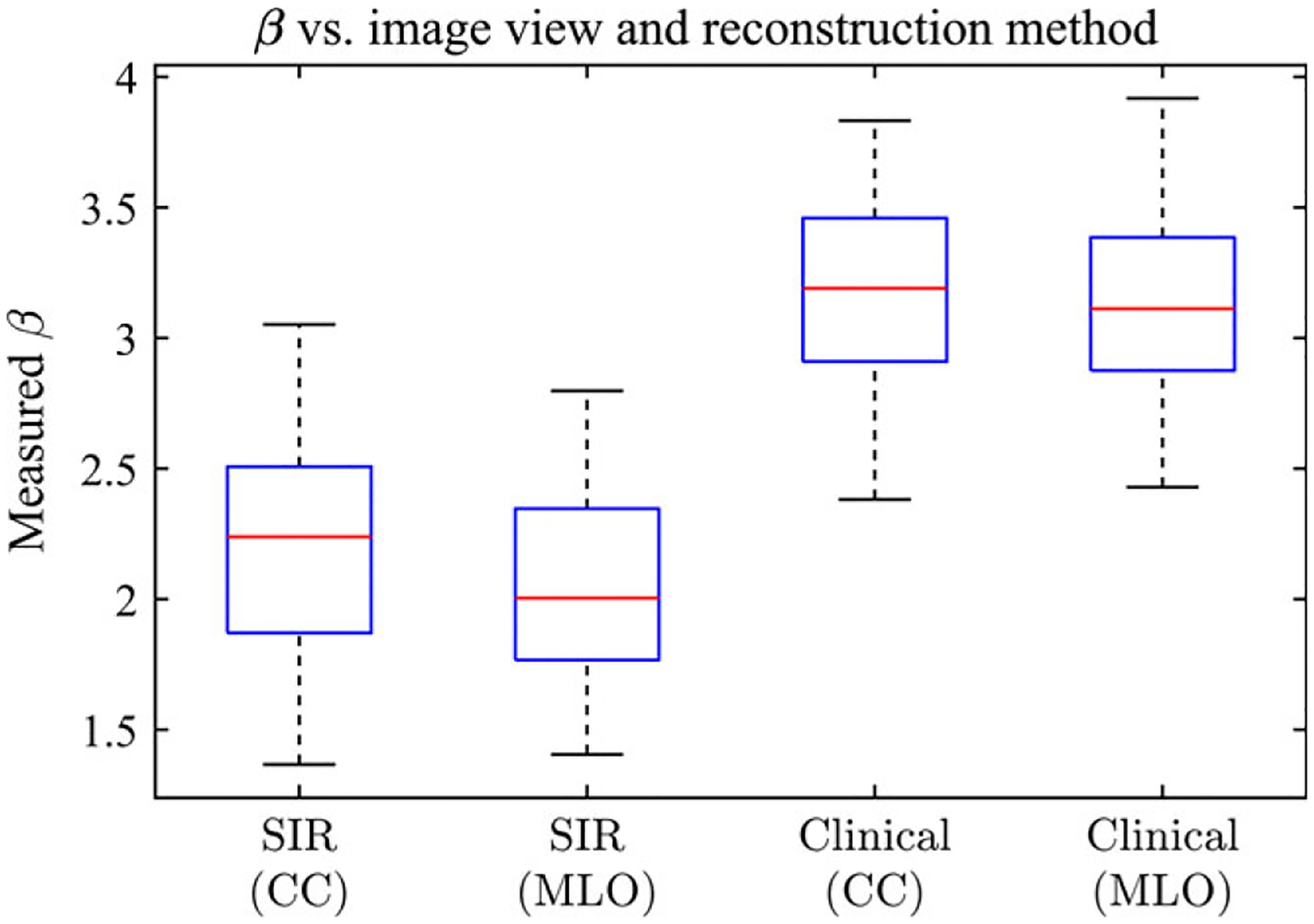
The measured β values for the DBT reconstructions shown separated by view.

4.C.4. Dependence on slice positions

Figure 13 shows the average β as a function of slice location for the central 25 slices about the center of the volume. These curves are relatively flat, indicating that, irrespective of reconstruction method, the anatomical clutter in the central slices about the center of the compressed breast is approximately the same. This was confirmed with the ANOVA comparison of the means, in which it was found that P > 0.05 for both reconstruction methods, indicating no statistically significant difference was present between the mean β values at different slice locations in either reconstruction method.

Fig. 13.

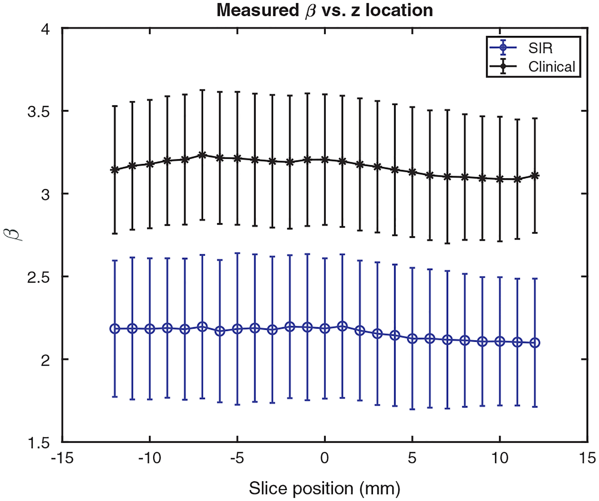
The average measured β value as a function of slice position for the two reconstruction methods.

5. DISCUSSION

In this work, the anatomical noise power spectra of DBT volumes generated using two reconstruction methods were measured and fitted to a power law model with two parameters, α and β. Image volumes of the same cohort of cases were reconstructed using each of the two methods and a direct comparison of the measured exponent β values was performed. Since the acquired data for the two reconstruction cohorts was the same, other parameters such as system geometry, acquisition parameters had no influence on the results. Under these conditions, it was found that the use of an SIR method reduced the through-plane artifacts levels and significantly reduced the anatomical clutter in DBT reconstructions as quantified using a power-law fitting of the anatomical noise power spectra. The measured β value is around 2.14 for SIR and 3.17 for the clinical reconstruction method. In addition, β had no significant dependence on either slice position or view (MLO vs CC) with either reconstruction method.

The measured β values in the clinical and SIR reconstructions were found to be moderately correlated (r² = 0.72, Fig. 11). This correlation indicates that a case with a small β value in one reconstruction method roughly corresponds to a small β value in the other. This result suggests that if measured β values are correlated with breast density, etc., in one reconstruction method, a similar correlation may be expected in the other. However, in Fig. 11, there are several outliers which lie closer to the line of slope unity than the other data points. Inspecting the reconstructed images for these outliers demonstrated that each of these four cases were fairly dense. In these outliers, it is possible that the anatomical clutter in both the clinical method and the SIR method are limited by the inherent anatomy in each slice, rather than the reconstruction method.

As shown by other investigators^16,19 and the result shown in this paper, the β values measured from the current clinical reconstruction is not significantly different from the β values measured from 2D mammography. Despite this minimal reduction in β, several large-scale clinical trials have shown that the introduction of DBT can help reduce recall rates, while simultaneously increasing cancer detection rates.^37,38 Given that even a slight reduction in the anatomical clutter may offer improved screening performance (recall our reference values of β = 3.235 and β = 3.080 for mammography and DBT, respectively), an immediate question to be answered in the future studies is the clinical implications of a significant reduction of anatomical clutter in the final outcome of clinical diagnoses. However, this question must be addressed in future clinical trial studies using much larger patient cohorts, rather than the relatively small cohort size used in this study. As a specific example, it has previously been shown¹⁴ that if quantum noise remains constant, but β is reduced, mass detection for human observers improves significantly with the most dramatic improvements for larger masses. An interesting question for future studies is to address what would be the impact of β parameter reduction in SIR on the mass detection tasks. Note that the use of SIR in DBT can result in a reduction of quantum noise level as well. Therefore, in the future, the impact of the SIR method on quantum noise should be explored and human observer studies should be used to validate this potential improvement in diagnostic performance and quantify the significance of any improvement.

Another potential significance of the reduced β values in SIR reconstructed DBT images can be inferred by the following consideration: with traditional mammography, it has been shown that anatomical clutter has a more pronounced impact on mass detection than quantum noise. As a result, the dependence of the images on dose is minimal,³⁹ unlike other well-known quantum-limited tomographic imaging systems such as computed tomography (CT).^40,41 Given the significantly reduced anatomical clutter in SIR-reconstructed DBT images, an interesting question arises: if the low-frequency power of the anatomical clutter is reduced, does the modality become more dose dependent? It would be interesting to investigate the potentially modified impact of radiation dose on diagnostic performance in DBT imaging with SIR reconstruction using model and human observer studies.

The SIR image reconstruction problem in Eq. (3) was solved in this work using the backward-forward splitting method together with variable splitting methods to convert the 2D TV denoising problem into a denoising problem with a generalized shrinkage operator as a solution. However, there are many other ways to solve the same optimization problem^42–49 including other strategies to leverage the elegance of a variety of other variable splitting method and corresponding ADMM update strategies^{42, 44,50–52} or to incorporate the benefits of TV regularization.^22,53–63

One potential limitation of this work is that we demonstrated through-plane blurring artifacts in DBT images could be reduced, resulting in a significant reduction in anatomical clutter when a specific SIR implementation is used; yet we have not demonstrated this can be achieved with other SIR methods in general. However, work from many other groups has previously shown that a reduction in through-plane blurring artifacts can be achieved using other SIR methods.^{21–23,58,64,65} Based upon our finding in this paper that the reduced anatomical clutter is associated with the reduction of through-plane blurring artifacts, it is anticipated that other SIR methods might also be used to reduce anatomical clutter as long as the parameters in these alternative methods are optimized to achieve the goal of through-plane artifacts reduction. Nevertheless, detailed studies in parameter selection for these methods and clinical studies similar to the one presented in this paper must be performed to answer the question of whether these methods can reduce anatomical clutter in the same way presented in this paper.

6. CONCLUSION

When SIR with proper reconstruction parameters was used to reconstruct DBT images, the width of the ASF in DBT was reduced by about 25% relative to that of the clinical reconstructions. Anatomical clutter characterized by the β values in anatomical noise power spectrum was reduced from β≈3.17 in clinical reconstruction to β≈2.14 in SIR.

APPENDIX. SOLVING THE DENOISING PROBLEM WITH 2D TV-NORM AS REGULARIZER

In this appendix, we present the detailed derivation of the used iterative solver of the denoising problem shown in Eq. (7):

$$\widehat{\tilde{x}}:=\underset{\tilde{x}}{\text{Arg\hspace{0.17em}Min}}[\frac{1}{2}{(\tilde{x}-u)}^T{P}^{-1}(\tilde{x}-u)+\lambda \sum _i\sqrt{{\left({\tilde{x}}_{i+1}-{\tilde{x}}_i\right)}^2+{\left({\tilde{x}}_{i+N}-{\tilde{x}}_i\right)}^2}]$$ (12)

The problem in Eq. (12) can be reformulated as the following constrained optimization problem with auxiliary variables d_i,x/y:²⁶

$$\begin{gathered} \widehat{\tilde{x}}=\underset{\tilde{x},d_{i,x},d_{i,y}}{\text{Arg\hspace{0.17em}Min}}\left\{\frac{1}{2}{(\tilde{x}-u)}^T{P}^{-1}(\tilde{x}-u)+\lambda \sum _i\sqrt{{\left(d_{i,x}\right)}^2+{\left(d_{i,y}\right)}^2}\right\} \\ \mathit{\text{s.t.\hspace{1em}}}{d}_{i,x}={\tilde{x}}_{i+1}-{\tilde{x}}_i,d_{i,y}={\tilde{x}}_{i+N}-{\tilde{x}}_i. \end{gathered}$$ (13)

This constrained optimization problem can then be solved by the minimization of augmented Lagrangian (AL) method via the ADMM algorithm.⁶⁶ Using the ADMM algorithm, the above TV minimization denoising is decomposed as the following three alternating sub-problems:

• X-Problem: The image variables, ${\tilde{x}}_i$, are updated at the iteration n+1 by minimizing the Augmented Lagrangian with the values of variables d and b at the iteration n as the input:

  $${\tilde{x}}_i^{n+1}:=\underset{{\tilde{x}}_i}{\text{Arg\hspace{0.17em}Min}}\left\{\frac{\lambda }{2p_i}{\left({\tilde{x}}_i-u_i\right)}^2+\frac{1}{2\mu }\left[{\left({\tilde{x}}_{i+1}^n-{\tilde{x}}_i-d_{i,x}^n-b_{i,x}^n\right)}^2+{\left({\tilde{x}}_{i+N}^n-{\tilde{x}}_i-d_{i,y}^n-b_{i,y}^n\right)}^2\right]\right\}.$$ (14)
• D-Problem: The introduced auxiliary variables d_i are updated at the iteration n+1 by minimizing the Augmented Lagrangian with input of variables ${\tilde{x}}_i$ at the iteration n+1 and the input of variables b at the iteration n:

  $$D_i^{n+1}:=\underset{d_i}{\text{Arg\hspace{0.17em}Min}}\sum _i\left\{\sqrt{{\left(d_{i,x}\right)}^2+{\left(d_{i,y}\right)}^2}+\frac{1}{2\mu }\left[{\left(d_{i,x}-e_{i,x}\right)}^2+{\left(d_{i,y}-e_{i,y}\right)}^2\right]\right\}.$$ (15)
  where

  $$e_{i,x}=b_{i,x}^n-\left({\tilde{x}}_{i+1}^{n+1}-{\tilde{x}}_i^{n+1}\right)$$ (16)

  $$e_{i,y}=b_{i,y}^n-\left({\tilde{x}}_{i+N}^{n+1}-{\tilde{x}}_i^{n+1}\right)$$ (17)
• B-problem: In ADMM scheme, the scaled multipliers b_i are updated using the following scheme:

  $$b_{i,x}^{n+1}=\left[d_{i,x}^{n+1}+e_{i,x}\right],$$ (18)

  $$b_{i,y}^{n+1}=\left[d_{i,y}^{n+1}+e_{i,y}\right].$$ (19)

The subproblems X and D can be readily solved with the following closed-from solutions.

• Solution of the X-Problem:

  $$\begin{gathered} {\tilde{x}}_i^{n+1}:=\frac{\mu /p_i}{\mu /p_i+4\lambda }{u}_i+\frac{4\lambda }{\mu /p_i+4\lambda }\left({\overline{x}}_i+h_i\right) \\ {\overline{x}}_i:=\frac{1}{4}\left({\tilde{x}}_{i+1}^n+{\tilde{x}}_{i+N}^n+{\tilde{x}}_{i-1}^n+{\tilde{x}}_{i-N}^n\right), \\ {h}_i:=\frac{1}{4}\left[\left(d_{i-1,x}^n-d_{i,x}^n\right)+\left(d_{i-N,y}^n-d_{i,y}^n\right)+\left(b_{i-1,x}^n-b_{i,x}^n\right)+\left(b_{i-N,y}^n-b_{i,y}^n\right)\right]. \end{gathered}$$ (20)

  These three formulae clearly dictate how the TV-denoising procedure works. The denoising result comes from two contributions: a weighted combination of the original image u_i and a denoised one, that is, ${\overline{x}}_i+h_i$. The weight for each component is $\frac{\mu /p_i}{\mu /p_i+4\lambda }$ and $\frac{4\lambda }{\mu /p_i+4\lambda }$, respectively. The smaller the λ values, the lower weight is assigned to the denoised contribution and vice versa. Moreover, the denoised image also consists of two terms: a low-pass filtered contribution ${\overline{x}}_i$ from a two-dimensional mean filter operation and a denoised edge contribution h_i which can be viewed as a high-pass operation.

• Solution of the D-Problem: the D-problem with two variables, d_i,x and d_i,y, can be easily solved and the result is written as follows using the well-known shrinkage operator S_μ(x):

  $$d_{i,x}^{n+1}=S_{\mu }\left(\left|E_i\right|\right)\frac{e_{i,x}}{\Vert E_i\Vert },d_{i,y}^{n+1}=S_{\mu }\left(\left|E_i\right|\right)\frac{e_{i,y}}{\Vert E_i\Vert }$$ (21)

  $$S_{\mu }(x)=x{\left(1-\frac{\mu }{\left|x\right|}\right)}_{+}=\{\begin{array}{l}x\left(1-\frac{\mu }{\left|x\right|}\right),\frac{\mu }{\left|x\right|}\in (0,1]\hfill \\ 0\hfill \end{array},$$ (22)

  Namely, the two components of variable D_i at each pixel are the shrinkage of the corresponding components of E_i variable with μ as the threshold reference: when ∣E_i ∣ < μ, both d_i,x and d_i,y are set to zero. Otherwise, both d_i,x and d_i,y are generated from the corresponding e_i,x and e_i,y by a fraction of (1 − μ/∣E_i∣).

REFERENCES

- 1.Ren B, Ruth C, Stein J, Smith A, Shaw I, Zhenxue J. Design and performance of the prototype full field breast tomosynthesis system with selenium based flat panel detector. Proc SPIE. 2005;5745:550–61. [Google Scholar]
- 2.Warner E Breast-cancer screening. N Engl J Med. 2011;365:1025–1032. [DOI] [PubMed] [Google Scholar]
- 3.Niklason LT, Christian BT, Niklason LE, et al. Digital tomosynthesis in breast imaging. Radiology. 1997;205:399–406. [DOI] [PubMed] [Google Scholar]
- 4.Niklason LT, Kopans DB, Hamberg LM. Digital breast imaging: tomosynthesis and digital subtraction mammography. Breast Disease. 1998;10:151–64. [DOI] [PubMed] [Google Scholar]
- 5.Dobbins III JT, Godfrey DJ. Digital x-ray tomosynthesis: current state of the art and clinical potential. Phys Med Biol. 2003;48:R65. [DOI] [PubMed] [Google Scholar]
- 6.Skaane P, Bandos AI, Gullien R, et al. Comparison of digital mammography alone and digital mammography plus tomosynthesis in a populationbased screening program. Radiology. 2013;267:47–56. [DOI] [PubMed] [Google Scholar]
- 7.Sechopoulos I A review of breast tomosynthesis. Part I. The image acquisition process. Med Phys. 2013;40:014301. [DOI] [PMC free article] [PubMed] [Google Scholar]
- 8.Caldwell CB, Stapleton SJ, Holdsworth DW, et al. Characterisation of mammographic parenchymal pattern by fractal dimension. Phys Med Biol. 1990;35:235. [DOI] [PubMed] [Google Scholar]
- 9.van der Schaaf A, van Hateren J. Modelling the power spectra of natural images: Statistics and information. Vision Res. 1996;36:2759–2770. [DOI] [PubMed] [Google Scholar]
- 10.Bochud FO, Verdun FR, Valley J-F, Hessler C, Moeckli R. Importance of anatomical noise in mammography. Proc SPIE. 1997;3036:74–80. [Google Scholar]
- 11.Bochud FO, Valley J-F, Verdun FR, Hessler C, Schnyder P. Estimation of the noisy component of anatomical backgrounds. Med Phys. 1999;26:1365–1370. [DOI] [PubMed] [Google Scholar]
- 12.Burgess AE, Jacobson FL, Judy PF. Human observer detection experiments with mammograms and power-law noise. Med Phys. 2001;28:419–437. [DOI] [PubMed] [Google Scholar]
- 13.Vedantham S, Shi L, Glick SJ, Karellas A. Scaling-law for the energy dependence of anatomic power spectrum in dedicated breast CT. Med Phys. 2013;40:011901. [DOI] [PMC free article] [PubMed] [Google Scholar]
- 14.Burgess AE, Judy PF. Signal detection in power-law noise: effect of spectrum exponents. J Opt Soc Am A. 2007;24:B52–B60. [DOI] [PubMed] [Google Scholar]
- 15.Metheany KG, Abbey CK, Packard N, Boone JM. Characterizing anatomical variability in breast CT images. Med Phys. 2008;35:4685–4694. [DOI] [PMC free article] [PubMed] [Google Scholar]
- 16.Chen L, Abbey CK, Nosratieh A, Lindfors KK, Boone JM. Anatomical complexity in breast parenchyma and its implications for optimal breast imaging strategies. Med Phys. 2012;39:1435–1441. [DOI] [PMC free article] [PubMed] [Google Scholar]
- 17.Chen L, Abbey CK, Boone JM. Association between power law coefficients of the anatomical noise power spectrum and lesion detectability in breast imaging modalities. Phys Med Biol. 2013;58:1663. [DOI] [PMC free article] [PubMed] [Google Scholar]
- 18.Barrett HH, Yao J, Rolland JP, Myers KJ. Model observers for assessment of image quality. PNAS. 1993;90:9758–9765. [DOI] [PMC free article] [PubMed] [Google Scholar]
- 19.Hu Y-H, Masiar M, Zhao W. Breast structural noise in digital breast tomosynthesis and its dependence on reconstruction methods. In: Marti J, Oliver A, Freixenet J, Marti R, eds. Digital Mammography, Lecture Notes in Computer Science. Vol. 6136, Berlin Heidelberg: Springer; 2010:598–605. [Google Scholar]
- 20.Vedantham S, Shi L, Karellas A, O’Connell AM. Conover D. Dedicated breast CT: anatomic power spectrum. Proc. of the Second International Conference on Image Formation in X-Ray Computed Tomography 2012:70. [Google Scholar]
- 21.Wu T, Moore RH, Rafferty EA, Kopans DB, A comparison of reconstruction algorithms for breast tomosynthesis. Med Phys. 2004;31:2636–2647. [DOI] [PubMed] [Google Scholar]
- 22.Sidky EY, Pan X, Reiser IS, Nishikawa RM. Moore RH, Kopans DB. Enhanced imaging of microcalcifications in digital breast tomosynthesis through improved image-reconstruction algorithms. Med Phys. 2009;36:4920–4932. [DOI] [PMC free article] [PubMed] [Google Scholar]
- 23.Xu S, Lu J, Zhou O, Chen Y. Statistical iterative reconstruction to improve image quality for digital breast tomosynthesis. Med Phys. 2015;42:5377–5390. [DOI] [PMC free article] [PubMed] [Google Scholar]
- 24.Sidky E, Pan X. Image reconstruction in circular cone-beam computed tomography by constrained, total-variation minimization. Phys Med Biol. 2008;53:4777. [DOI] [PMC free article] [PubMed] [Google Scholar]
- 25.Combettes PL, and Wajs VR. Signal recovery by proximal forward-backward splitting. SIAM Multiscale Model Simul. 2005;4:1168–1200. [Google Scholar]
- 26.Wang Y, Yang J, Yin W, Zhang Y. A new alternating minimization algorithm for total variation image reconstruction. SIAM J Imag Sci. 2008;1:248–272. [Google Scholar]
- 27.Hudson HM, Larkin RS. Accelerated image reconstruction using ordered subsets of projection data. IEEE Trans Med Imag. 1994;13:601–609. [DOI] [PubMed] [Google Scholar]
- 28.Thibault J-B, Bouman CA, Sauer KD, Hsieh J. A recursive filter for noise reduction in statistical iterative tomographic imaging. Proc SPIE. 2006;6065:6065–6065–10. [Google Scholar]
- 29.Zhang R, Thibault JB, Bouman CA, Sauer KD, Hsieh J. Model-based iterative reconstruction for dual-energy X-Ray CT using a joint quadratic likelihood model. IEEE Trans Med Imag. 2014;33:117–134. [DOI] [PubMed] [Google Scholar]
- 30.Zhang Y, Chan H-P, Sahiner B, et al. Application of boundary detection information in breast tomosynthesis reconstruction. Med Phys. 2007;34:3603–13. [DOI] [PMC free article] [PubMed] [Google Scholar]
- 31.Zhang Y, Chan H-P, Wu Y-T, et al. Truncation artifact and boundary artifact reduction in breast tomosynthesis reconstruction. Proc SPIE. 2008;6913:69132Y. [Google Scholar]
- 32.Navab N, Bani-Hashemi A, Nadar MS, et al. 3D reconstruction from projection matrices in a C-arm based 3Dangiography system. In: Wells WM, Colchester A, Delp S, eds. MICCAI’98: First International Conference Cambridge, MA, USA, October 11–13, 1998 Proceedings. Berlin, Heidelberg: Springer; 1998;119–129. [Google Scholar]
- 33.Hu Y-H, Zhao B, Zhao W. Image artifacts in digital breast tomosynthesis: investigation of the effects of system geometry and reconstruction parameters using a linear system approach. Med Phys. 2008;35:5242–5252. [DOI] [PMC free article] [PubMed] [Google Scholar]
- 34.Strudley CJ, Young KC, Looney P, Gilbert FJ. Development and experience of quality control methods for digital breast tomosynthesis systems. Br J Radiol. 2015;88:20150324. [DOI] [PubMed] [Google Scholar]
- 35.Rodríguez-Ruiz A, Castillo M, Garayoa J, Chevalier M. Evaluation of the technical performance of three different commercial digital breast tomosynthesis systems in the clinical environment. Phys Med. 2016;32:767–777. [DOI] [PubMed] [Google Scholar]
- 36.Garrett J, Ge Y, Li K, Chen G-H. Anatomical background noise power spectrum in differential phase contrast and dark field contrast mammograms. Med Phys. 2014;41:120701. [DOI] [PubMed] [Google Scholar]
- 37.Rafferty EA, Durand MA, Conant EF, et al. Breast cancer screening using tomosynthesis and digital mammography in dense and nondense breasts. JAMA 2016;315:1784–1786. [DOI] [PubMed] [Google Scholar]
- 38.Friedewald SM, Rafferty EA, Rose SL, et al. Breast cancer screening using tomosynthesis in combination with digital mammography. JAMA 2014;311:2499–2507. [DOI] [PubMed] [Google Scholar]
- 39.Ruschin M, Timberg P, Båth M, et al. Dose dependence of mass and microcalcification detection in digital mammography: free response human observer studies. Med Phys. 2007;34:400–407. [DOI] [PMC free article] [PubMed] [Google Scholar]
- 40.Silverman JD, Paul NS, Siewerdsen JH. Investigation of lung nodule detectability in low-dose 320-slice computed tomography. Med Phys. 2009;36:1700–1710. [DOI] [PMC free article] [PubMed] [Google Scholar]
- 41.Saiprasad G, Filliben J, Peskin A, et al. Evaluation of low-contrast detectability of iterative reconstruction across multiple institutions, CT scanner manufacturers, and radiation exposure levels. Radiology. 2015;277:124–133. [DOI] [PubMed] [Google Scholar]
- 42.Chun SY, Dewaraja YK, Fessler JA. Alternating direction method of multiplier for tomography with nonlocal regularizers. IEEE Trans Med Imag. 2014;33:1960–1968. [DOI] [PMC free article] [PubMed] [Google Scholar]
- 43.Zheng J, Fessler JA, Chan HP. Detector blur and correlated noise modeling for digital breast tomosynthesis reconstruction. IEEE Trans Med Imag. 2017;37:116–127 [DOI] [PMC free article] [PubMed] [Google Scholar]
- 44.Ramani S, Fessler JA. A splitting-based iterative algorithm for accelerated statistical x-ray CT reconstruction. IEEE Trans Med Imag. 2012;31:677–688. [DOI] [PMC free article] [PubMed] [Google Scholar]
- 45.Zheng J, Fessler JA, Chan H-P. Segmented separable footprint projector for digital breast tomosynthesis and its application for subpixel reconstruction. Med Phys. 2017;44:986–1001. [DOI] [PMC free article] [PubMed] [Google Scholar]
- 46.Zheng J, Fessler JA, Chan H-P. Effects of detector blur and correlated noise on digital breast tomosynthesis reconstruction. Proc SPIE. 2017;10132:10132–10137. [DOI] [PMC free article] [PubMed] [Google Scholar]
- 47.Zheng J, Fessler JA, Chan H-P. Digital breast tomosynthesis reconstruction using spatially weighted non-convex regularization. Proc SPIE. 2016;9783:7. [Google Scholar]
- 48.Lu Y, Chan H-P, Fessler JA, Hadjiiski L, Wei J, Goodsitt MM. Adaptive diffusion regularization for enhancement of microcalcifications in digital breast tomosynthesis (DBT) reconstruction. Proc SPIE. 2011;7961:9. [DOI] [PMC free article] [PubMed] [Google Scholar]
- 49.Lu Y, Chan H-P, Wei J, Hadjiiski LM. Selective-diffusion regularization for enhancement of microcalcifications in digital breast tomosynthesis reconstruction. Med Phys. 2010;37:6003–6014. [DOI] [PMC free article] [PubMed] [Google Scholar]
- 50.Nien H, Fessler JA. Fast x-ray CT image reconstruction using a linearized augmented lagrangian method with ordered subsets. IEEE Trans Med Imag. 2015;34:388–399. [DOI] [PMC free article] [PubMed] [Google Scholar]
- 51.McGaffin MG, Fessler JA. Alternating dual updates algorithm for x-ray CT reconstruction on the GPU. IEEE Trans Comp Imag. 2015;1:186–199. [DOI] [PMC free article] [PubMed] [Google Scholar]
- 52.Nien H, Fessler JA, Relaxed linearized algorithms for faster x-ray CT image reconstruction. IEEE Trans Med Imag. 2016;35:1090–1098. [DOI] [PMC free article] [PubMed] [Google Scholar]
- 53.Sidky EY, Reiser I, Nishikawa RM, et al. Practical iterative image reconstruction in digital breast tomosynthesis by non-convex TpV optimization. Proc SPIE. 2008;6913:6. [Google Scholar]
- 54.Jang KE, Sung Y, Lee K, Lee J, Cho S. Statistical reconstruction using dual formulation of subband-wise total variation regularization (SDST) for limited angle tomography. 2011 IEEE International Symposium on Biomedical Imaging: From Nano to Macro; 2011:1762–1765. [Google Scholar]
- 55.Jang KE, Sung Y, Lee K, Lee J, Cho S. Limited data tomographic image reconstruction via dual formulation of total variation minimization. Proc SPIE. 2011;79617961–7968 [Google Scholar]
- 56.Sidky EY, Duchin Y, Reiser I, Ullberg C, Pan X. Optimizing algorithm parameters based on a model observer detection task for image reconstruction in digital breast tomosynthesis. In: 2011 IEEE Nuclear Science Symposium Conference Record; 2011:4230–4232. [Google Scholar]
- 57.Ertas M, Yildirim I, Kamasak M, Akan A. Digital breast tomosynthesis image reconstruction using 2D and 3D total variation minimization. Biomed Eng Online. 2013;12:112. [DOI] [PMC free article] [PubMed] [Google Scholar]
- 58.Vengrinovich VL, Zolotarev SA, Linev VN. Experimental investigation of iterative reconstruction techniques for high resolution mammography. AIP Conference Proceedings. 2014;1581:1808–1815. [Google Scholar]
- 59.Mota AM, Matela N, Oliveira N, Almeida P. Total variation minimization filter for DBT imaging. Med Phys. 2015;42:2827–2836. [DOI] [PubMed] [Google Scholar]
- 60.Mota AM, Oliveira N, Almeida P, Matela N. 3D total variation minimization filter for breast tomosynthesis imaging. In: Tingberg A, Lång KL, Timberg P, eds. Breast Imaging, Cham: Springer International Publishing; 2016:501–509. [Google Scholar]
- 61.Kim K, Park Y, Cho H, et al. Improvement of image performance in digital breast tomosynthesis (DBT) by incorporating a compressed-sensing (CS)-based deblurring scheme. Radiat Phys Chem. 2016;127:147–154. [Google Scholar]
- 62.Piccolomini EL, Morotti E. A fast total variation-based iterative algorithm for digital breast tomosynthesis image reconstruction. J Algorithm Comput Technol. 2016;10:277–289. [Google Scholar]
- 63.Zhang J, Hu Y, Nagy JG. A scaled gradient method for digital tomographic image reconstruction. Inverse Probl Imaging. 2017;12:239–259. [Google Scholar]
- 64.Rakowski JT, Dennis MJ. A comparison of reconstruction algorithms for C-arm mammography tomosynthesis. Med Phys. 2006;33:3018–3032. [DOI] [PubMed] [Google Scholar]
- 65.Zhang Y, Chan H-P, Sahiner B, et al. A comparative study of limited-angle cone-beam reconstruction methods for breast tomosynthesis. Med Phys. 2006;33:3781–3795. [DOI] [PMC free article] [PubMed] [Google Scholar]
- 66.Boyd S, Parikh N, Chu E, Peleato B, Eckstein J. Distributed optimization and statistical learning via the alternating direction method of multipliers. Found Trends Mach Learn. 2011;3:128. [Google Scholar]