Conformational Optimization with Natural Degrees of Freedom: A Novel Stochastic Chain Closure Algorithm

Abstract

The present article introduces a set of novel methods that facilitate the use of “natural moves” or arbitrary degrees of freedom that can give rise to collective rearrangements in the structure of biological macromolecules. While such “natural moves” may spoil the stereochemistry and even break the bonded chain at multiple locations, our new method restores the correct chain geometry by adjusting bond and torsion angles in an arbitrary defined molten zone. This is done by successive stages of partial closure that propagate the location of the chain break backwards along the chain. At the end of these stages, the size of the chain break is generally reduced so much that it can be repaired by adjusting the position of a single atom. Our chain closure method is efficient with a computational complexity of O(N_d), where N_d is the number of degrees of freedom used to repair the chain break. The new method facilitates the use of arbitrary degrees of freedom including the “natural” degrees of freedom inferred from analyzing experimental (X-ray crystallography and nuclear magnetic resonance [NMR]) structures of nucleic acids and proteins. In terms of its ability to generate large conformational moves and its effectiveness in locating low energy states, the new method is robust and computationally efficient.

1. INTRODUCTION

Conformational optimization of biomolecular structure is widely used both in computational modeling and in the refinement of experimental measurements derived from X-ray crystallography and nuclear magnetic resonance (NMR) spectroscopy. Any conformational optimization protocol requires an energy function, an optimization algorithm, and a set of independent degrees of freedom. The choice of the energy function depends on a particular application that may model a biomolecular structure at coarse grain or at full atomic detail. As our findings are independent of the particular energy function, we focus on optimization algorithms and especially on the choice of degrees of freedom.

The choice of optimization algorithm has a significant effect on the quality of the generated conformations giving rise to a demand for fast and accurate conformational optimization algorithms with widespread applicability. Energy minimization methods such as the conjugate gradient (Hestenes and Stiefel, 1952) or the truncated Newton (Schlick and Overton, 1987) methods are well suited for finding a conformation that corresponds to a local minimum of the energy surface. Locating the global minimum conformation is generally better achieved by simulated annealing type methods (Kirkpatrick et al., 1983; Nayeem et al., 1991). In order to find a diverse set of local minimum conformations, either Monte Carlo minimization (MCM) (Li and Scheraga, 1987; Wales and Scheraga, 1999; Brooks et al., 2001) or stochastic tunneling (Barhen et al., 1997) is preferred. If the aim is to generate ensembles of conformations around each local minimum, then both molecular dynamics (Voter, 1997; Minary et al., 2003, 2004) and Monte Carlo (Metropolis et al., 1953; Swedensen and Wang, 1987; Tanner and Wong, 1987) based methods can be used. The robustness and performance of all the above algorithms can be significantly improved by methods that involve multiple replicas (Geyer, 1991; Kou et al., 2006; Minary and Levitt, 2006) of the system, smoothing transformation (Rahman and Tully, 2002a,b) of the energy surface and global reformulation of the classical partition function (Minary et al., 2008).

The choice of degrees of freedom is also critically important in global optimization but has received less attention. Two sets of degrees of freedom used from the earliest days of biomolecular modeling are the atomic Cartesian coordinate and the single-bond torsion angles. Torsion angles were used first on small peptides as a way to combat the many degrees of freedom of these systems (Gibson and Scheraga, 1967a,b). Soon afterwards, Cartesian coordinates were used in the first all-atom energy minimization of an entire protein (Levitt and Lifson, 1969). While useful for energy minimization, the large number of Cartesian degrees freedom (3 times the number of atoms) makes any conformational search practically intractable. Torsion angle coordinates are more economical with about 4 single-bond torsion angles per amino acid residue on average. Unfortunately, conventional Markov Chain Monte Carlo algorithms (Metropolis et al., 1953) have a very slim chance of accepting a torsional move in a long all-atom biomolecular chain. The problem, which is caused to the long lever arm moving atoms distant from the bond about which the rotation is applied, can be partially circumvented by local torsional moves applied to a segment of the molecule while the rest of the system is kept fixed. The most widespread method in this category is CONROT (Dodd et al., 1993), but there are several alternative approaches such as symmetric (Krishna and Theodoru, 1995) or analytical rebridging (Wu and Deem, 1999), window moves (Hoffmann and Knapp, 1996), and various modifications of the original CONROT method (Umschneider and Jorgensen, 2003). A common result of such local moves is that the polypeptide chain becomes broken; this then needs to be fixed by solving chain closure equations numerically at considerable computational cost. Recently, a new computationally more efficient constant bond length closure algorithm has been proposed by Sklenar et al. (2006); it works by adjusting the position of a common bridging atom and changing corresponding bond and torsion angles so that broken bond lengths are restored. These and former studies by Umschneider and Jorgensen (2003) showed that augmenting torsional with bond-angle space leads to a significant softening of the energy landscape.

In this article, we introduce a new chain breakage and closure method that allows us to use arbitrary degrees of freedom for conformational optimization of biomolecular structures. Thanks to its modest computational cost and its ability to handle arbitrary large chain breaks, our approach combines the beneficial features of the best currently used methods. In our approach, chain breaks caused by independent moves of arbitrary type (for both proteins and nucleic acids) and magnitude can still be restored by adjusting a sufficient number of torsion and bond angles. Furthermore, moves based on our new chain breakage-closure method can be incorporated into any advanced sampling/optimization protocol (Geyer, 1991; Kou et al., 2006; Minary and Levitt, 2006; Rahman and Tully, 2002a,b; Minary et al., 2008). In the present study, we have chosen to use conventional Metropolis Monte Carlo (Metropolis et al., 1953) as our conformational search tool. In this way, improvement in computational efficiency is exclusively a result of our new algorithm.

Our results show that our new stochastic approach is one of the simplest, cheapest, and at the same time, most robust of current closure-based algorithms. In particular, it can restore an order of magnitude larger chain breaks than other closure algorithms at comparable computational cost. Combining collective natural moves and our stochastic closure leads to very efficient conformational optimization protocols that locate conformational energy minima not easily found by other chain closure or torsional sampling algorithms.

2. METHODS

2.1. Stochastic partial closure

The central part of our method is called Stochastic Partial Closure (SPC). It is better than the previously used Deterministic Full Closure (DFC) approach by Sklenar et al. (2006) in that it always provides a solution to the closure problem. More specifically, under certain conditions, DFC provides a favorable solution, but otherwise it provides no solution (Fig. 1a).

FIG. 1.

(a) Two-dimensional illustration of Deterministic Full Closure (DFC) applied to a five-atom chain r₁, …, r₅ with a broken bond between atom 4 and 5. If atom 4 is to be positioned by changing the bond angle defined by atoms 2-3-4, then there will either be one favorable solution (marked as point A) or else no solution. (b) Showing Stochastic Partial Closure (SPC) applied to the problem in (a). We mark, S, the red circular arc of constant bond length around atom 5 (a surface in 3D), and IP, the intersection point of the arc S and the line connecting atom 4 to 5. SPC stochastically places atom 4 on arc S based on a normal distribution centered on IP. This method always gives a solution, although it may stretch the bond between atoms 3 and 4. (c) Showing one cycle of Recursive Stochastic Closure (RSC) consisting of three successive, recursive stages of SPC and a single terminating stage of DFC. Circles and lines colored in gray mark atoms and bonds set by SPC, whereas circle and line in green mark atoms and bonds set by the final DFC stage. The figure shows how RSC adjusts bond angles (in 3D, both torsion and bond angles are adjusted), so that the chain break is repaired. The right-most atom is the head atom, which is on the other side of the break; the two left-most atoms belong to the anchor. The other atoms are molten zone.

The algorithm

Given four consecutively connected atoms, r₁, …, r₄, an arbitrarily positioned fifth atom, r₅ and a desired value for the bond length d₄₅, SPC proceeds as follows (Fig. 1b): (i) Define a line (a) that connects atoms 4 and 5. (ii) Find the intersection point (IP) between line a and a sphere of radius d₄₅ centered on atom r₅. (iii) At the intersection point, construct a plane (S^T) tangential to surface S. (iv) Choose a random point P^T on the tangential surface, S^T, using a two-dimensional normal distribution, N₂ (μ, Σ) with mean l μ = (x_IP, y_IP) and standard deviation, (Σ₁₁, Σ₂₂) = (σ_spc, σ_spc). (v) Obtain the new position of atom 4 by projecting P^T onto the spherical surface, S.

In the absence of the chain break, SPC done with σ_spc = 0 leaves the conformation unchanged, whereas SPC done with σ_spc > 0 may still produce a new position for atom 4. In further context, both SPC and DFC also refer to a unary operator that acts on the conformation of a single atom.

2.2. Recursive stochastic closure

Consider a segment of an atomic chain and the next chain atom called the “head.” Recursive Stochastic Closure (RSC) repairs a broken connection between the terminal atom of the segment and the fixed head atom by distributing a bond length preserving deformation along the segment. The segment region that participates in the deformation is called the molten zone whose atoms are numbered from 1 to N_m. Atom 1 is adjacent to the head atom. Succeeding atom N_m, the segment has at least two more “anchor” atoms that do not participate in the deformation.

The algorithm

Consider a molten zone with N_m = n + 1 atoms r₁, …, r_n+1, an arbitrarily positioned head atom r_h and two anchor atoms, r_n+2, r_n+3 which are continuation of the molten zone along the segment. One RSC cycle combines n recursively executed SPC steps that update the position of the first n atoms of the molten zone followed by a final step of DFC that determines the new position of atom n + 1. When RSC is defined as a unary operator that operates on the conformation to the right, the full cycle can be expressed as: RSC(σ_spc) = DFC · SPC_n(σ_spc) · SPC_n−1(σ_spc) … · SPC₁(σ_spc). Here, SPC₁(σ_spc) repairs the broken connection between atom 1 and the head atom, SPC_i(σ_spc) connects atoms i and i − 1 and DFC terminates the cycle by setting bond angle at atom n + 2.

When RSC is used with σ_spc = 0, it acts like a projection onto the surface of constant bond length. When RSC is used with σ_spc > 0, then the chain break is repaired (Fig. 1c) and bond and torsion angles are changed by randomly changing atomic positions along the molten zone. Thus, repeated applications of RSC will produce a series of different conformations for the molten zone. Our algorithm is flexible in that it allows the use of any kind of DFC following after a recursive sequence of an arbitrary number of SPC steps. In this article, we always use the cost-effective algorithm described in Sklenar et al. (2006) for DFC. Note that the value of n depends on the geometry of the system under consideration.

Implementation of the algorithm

Assuming that the final DFC step always have a solution, the following code segment outlines the set of instructions used to perform a single RSC cycle that repairs the chain break by resetting the position of atoms in the molten zone.

	subroutine rsc(MG, i)
1.	if i = 1
2.	ri ← (spc)[ri, rh]
3.	else
4.	ri ← (spc)[ri, ri−1]
5.	if i < n + 1
6.	call rsc(MG, i + 1)
7.	else
8.	rn+1 ← (dfc)[rn+3, rn+2, rn+1, rn]

One of the arguments of subroutine “rsc” is the atomic index, i that monitors the internal progress of the RSC cycle. Prior to calling “rsc,” initial condition i = 1 is set so that the cycle starts with the first atom of the molten zone. The other argument, group ^MG holds the coordinates of molten zone, head, and anchor atoms. The referenced functions, “spc” and “dfc,” implement one step of SPC and DFC, respectively. Besides, both of these functions return the modified conformation of a single atom. Subroutine “rsc” is called recursively until the chain break is repaired.

Lemma 1

Given that N_d is the number of dependent degrees of freedom changed by an RSC cycle, the asymptotic cost of the chain closure problem is ½ c_spc O(N_d), where c_spc is the number of operations used in one SPC step.

Proof

The number of operations used to perform one RSC cycle involving n SPC steps is n c_spc + c_dfc, where c_spc and c_dfc are the number of operations in one SPC and DFC steps, respectively. Therefore, the asymptotic cost of one RSC cycle is O(n c_spc + c_dfc) = c_spc O(n). By altering the position of all N_m atoms in the molten zone, one RSC cycle changes the value of N_m + 2 bond angles and N_m + 3 torsion angles. Therefore, N_d = 2 N_m + 5 = 2 (n + 1) + 5. Thus, c_spc O(n) = c_spc. O(½ (N_d − 5) − 1) = ½c_spc O(N_d).

2.3. Monte Carlo recursive stochastic closure

The algorithm

Consider any molecular assembly which is divided into independent structural segments that upon rearrangement may cause chain breaks at different locations in the system. Each of these locations has a molten zone. One step of Monte Carlo Recursive Stochastic Closure (MCRSC) starts with an arbitrary random move that rearranges the structural segments and causes chain breaks. These chain breaks are then repaired by applying m cycles of RSC to all the molten zones. The first RSC cycle attempts to repair the chain break by a simple geometric closure, which may not satisfy local stereochemistry. If any of the first RSC cycles fail, the step is rejected. If all succeed then each additional RSC cycle move is accepted according to the Metropolis criterion using an energy function that measure bond and torsion angle strain. In this way each additional RSC cycle move attempts to find a closure that is energetically more favorable than the one found by the preceding cycle. Thus, a conformation for each molten zone is found so that all the associated torsion and bond angles are strain free. Finally, the resulting chain break free conformation is also accepted according to the Metropolis criterion, but this time the complete energy function of the system is used. Thus, there is only one costly energy evaluation per step, which may also involve many low-cost RSC cycles that attempt to find an energetically favorable chain closure.

Implementation of the algorithm

Considering that X, which denotes all degrees of freedom of a molecular assembly, is divided into independent, X_i, and dependent, X_d, variables, the use of MCRSC is demonstrated by the following program.

	program mcrsc
1.	Ea ← E[X]
2.	for imc ← 1 to Nmc do
3.	sX ← X
4.	call update_idof(Xi)
5.	call general_rsc(Xd)
6.	dEa ← dE[Xd]
7.	for irsc ← 1 to m − 1 do
8.	sXd ← Xd
9.	call general_rsc(Xd)
10.	dEp ← dE[Xd]
11.	pa ← exp[ − β (dEp − dEa)]
12.	if min[1, pa] > y ∈ U(0, 1)
13.	dEa ← dEp
14.	else
15.	Xd ← sXd
16.	Ep ← E[X]
17.	pa ← exp[− β (Ep − Ea)]
18.	if min[1, pa] > y ∈ U(0, 1)
19.	Ea ← Ep
20.	else
21.	X ← sX

This program performs N_mc MCRSC steps and uses the following key functions and variables: (1) Function E[…] takes argument X and returns the energy score for the whole system. (2) Function ^dE[…] takes argument ^dX and returns the energy associated with the state of all bond and torsion angles that are used to solve chain breaks. (3) Variables E_p and E_a hold the energy score of proposed and accepted conformations. (4) Variables ^dE_p and ^dE_a hold the energy score returned by function ^dE[…] for proposed and accepted closure states. (5) In one-dimensional arrays ^sX and ^sX_d, the state of X and X_d are saved. At the beginning of each MCRSC step all independent degrees of freedom are updated (line 4) by subroutine update_idof, which is defined in Section 7.1. This is followed by one cycle of RSC by subroutine general_rsc that updates all dependent degrees of freedom and repairs all chain breaks. This subroutine is presented in Section 7.2. The following, m − 1 RSC cycles drive an encapsulated Monte Carlo scheme (lines 7–15) guided by cheaply evaluated energy function ^dE[…]. This leads to conformational relaxation along dependent variables so that energetically favorable chain closures are found. Further conformational relaxation along dependent variables may be achieved by simulated annealing. Finally, the energy score of the new proposed conformation, X is evaluated (line 16) and X is accepted (lines 17–21) according to the Metropolis criterion. In theory, we could choose such a large move size along the independent variables so that some of the chain breaks may not be repaired due to the lack of a geometric solution (line 5). While not indicated explicitly, in this case the whole step is rejected.

Lemma 2

Consider a molecular assembly that has N_c chain breaks and adjacent molten zones. If N_d is the number of dependent degrees of freedom, the asymptotic cost of applying an RSC cycle to all the molten zones is ½ c_spc O(N_d) + c_dfc O(N_c), where c_spc and c_dfc are the costs of a single SPC and DFC steps, respectively.

Proof

See the Appendix.

Lemma 3

Consider the molecular assembly of Lemma 2 with N atoms. For any value of N_c and N_d, the asymptotic cost of applying an RSC cycle to all the molten zones has an upper bound (1.5 c_spc + c_dfc)O(N), where c_spc and c_dfc are the costs of single SPC and DFC steps.

Proof

See the Appendix.

Corollary 1

Assume that c_eO(N) is the asymptotic cost of the total energy calculation in an N atom system. For any N_c and N_d, the asymptotic cost of repairing all chain breaks by RSC cycles does not exceed the asymptotic cost of the energy calculation. If both N_c and N_d are orders of magnitude smaller than N (e.g., the present applications), the total energy calculation will dominate the cost of an MCRSC step.

Comparison with other methods

Given that for every new state of the independent degrees of freedom the dependent degrees of freedom (chain closure variables) are relaxed, MCRSC is equivalent to Metropolis Monte Carlo sampling guided by the function,

$$\stackrel{\sim }{E}(X)=\stackrel{\sim }{E}(X_i\cup X_d)=\underset{X_d}{min}\{E(X_i\cup X_d)\}.$$ (1)

Our new method is similar to the MCM technique reviewed in Wales and Scheraga (1999) in which the Monte Carlo sampling is guided by the transformed energy function

$$\stackrel{\sim }{E}(X)=\underset{X}{min}\{E(X)\}$$ (2)

where min refers to minimization along X. This transformation preserves all local minima and also leads to an energy surface Ẽ (X) that can be efficiently explored by using Monte Carlo as described in Metropolis et al. (1953).

2.4. Using Monte Carlo recursive stochastic closure for nucleic acids

Figure 2 illustrates MCRSC for nucleic acid structure using the rigid-body motion of the base pairs as the natural variables. In Figure 2a, RSC repairs a chain break between two nucleotides by randomly adjusting the positions of atoms in the molten zone. The number of atoms in molten zone, N_m determines the number of SPC steps in each RSC cycle, n = N_m − 1, because one atom is always moved by DFC. In this study, each molten zone of all-atom nucleic acids is composed of three (N_m = 3) consecutive atoms P, O5′, and C5′. Therefore, in each RSC cycle, the number of SPC steps n = N_m − 1 = 2. Unless otherwise noted, randomness was introduced by setting σ_spc = 10⁻⁴ Å and we used five consecutive RSC cycles (m = 5) in each MCRSC step.

FIG. 2.

Illustration of how our Monte Carlo Recursive Stochastic Closure (MCRSC) algorithm works on a simple example of a dinucleotide. (a) Conformational space is drawn as a function of bond lengths, bond angles and torsion angle rotations. The starting state, O, is moved towards point A causing a break in the molecular chain. The break is repaired by one cycle of Recursive Stochastic Closure (RSC) that adjusts the conformation of the molten zone comprising atoms P, O5′, and C5′ (N_m = 3). The first two SPC stages, A→B & B→C, which move atoms P and O5′, are followed by a DFC stage, C→D_{m = 1}, placing atom C5′. The cycle is then repeated to relax chain stiffness between atoms O3′ and C4′ to reach point D_{m = 2}. (b) Showing how we deal with degrees of freedom in nucleic acids. The dotted black lines mark chain breaks that can be caused by Monte-Carlo moves in the independent variables, X_i (marked in brown). After closing the furanose ring (RC) by adjusting the position of atom C4′, RSC repairs the chain break while setting the value of dependent variables, X_d: torsion angles (magenta) and bond angles at every atom of the chain connecting nucleotides. There are 10 independent degrees of freedom per nucleotide: 12 “structural” degrees of freedom describing the relative orientations of bases (each counts as ½ as two nucleotides share each degree of freedom) and 4 variables of the ribose ring. The “structural” degrees of freedom are Shear (S_x), Stretch (S_y), Stagger (S_z), Buckle (κ), Propeller (π), Opening (σ), Shift (D_x), Slide (D_y), Rise (D_z), Tilt (τ), Roll (ρ), and Twist (ω).

The ten independent degrees of freedom, X_i, of each nucleotide in a DNA double helix are depicted in Figure 2b. Here, six out of ten degrees of freedom are responsible for the global orientation of nucleotides and four provide the internal flexibility of the furanose ring. Unless explicitly noted, the move sizes (see Section 6.3) of independent natural degrees of freedom were set to σ = 2.5×10⁻⁵ Å for translational, σ = 10⁻⁵ radian for rotational and internal angle moves. In addition to breaking the chain along the P – O3′ bond, changes in the independent degrees of freedom may also break the furanose ring bond C4′ – O1′; this ring break is always restored by DFC.

2.5. Using Monte Carlo recursive stochastic closure for proteins

The molten zones are located along loops between structural segments. Here, we place the chain break within the residue that marks the starting point of molten zones which include three additional residues. Because we use two backbone atoms per residue in our protein representation (see Section 6.2), the molten zones consist of N_m = 2×3 + 1 = 7 atoms. Thus, the number of SPC steps per RSC cycle, n = N_m − 1 = 6. Randomness was modeled by σ_spc = 10⁻⁴ Å, and we used five RSC cycles (m = 5) in each MCRSC step.

Sets of independent degrees of freedom, X_i, for the relative orientation of segment pairs composed of two rigid β-sheets, two α-helices and an α-helix with a β-sheet are shown in Figure 3a–c. Here, the move sizes (see Section 6.3) of independent degrees of freedom were set to σ = 10⁻⁴ Å for translational and σ = 10⁻⁵ radian for rotational moves.

FIG. 3.

Natural degrees of freedom that are used on protein structure. (a) A sandwich of two three-stranded anti-parallel β-sheets (β-strands are shown as rectangular slabs) with natural degrees of freedom that treat the β-sheets as rigid bodies. These independent variables, X_i are Shift (D_x), Slide (D_y), Rise (D_z), Tilt (τ), Roll (ρ), and Twist (ω). (b) Two rigid helical segments (α-helices are shown as cylinders) with the natural degrees of freedom that describe their relative orientation. These independent variables, X_i, are Shear (S_x), Stretch (S_y), Stagger (S_z), Buckle (κ), Propeller (π), and Opening (σ). (c) Illustration of the move along Shear (S_x), one of the natural degrees of freedom describing the relative orientation of a three-stranded β-sheet and an α-helix. All the remaining independent variables, X_i, are identical to the ones in (b) and can be derived if one aligns the α-helix with the central strand of the β-sheet. (d) Showing one possible arrangement of the flexible protein loops (dashed line) that connect individual β-strands and α-helices. The red rectangle illustrates a loop segment containing a molten zone with N_m = 7 between magenta atoms. Recursive Stochastic Closure (RSC) changes the conformation of the molten zone, so that the broken connection between segments (β-strands, α-helices) is repaired. In the lack of torsion or bond angle constraints (e.g., peptide planes are not described explicitly in coarse grain representation), there are 19 dependent degrees of freedom, X_d (magenta).

3. RESULTS

3.1. Robust handling of chain breakages in nucleic acids

We investigated how the proposed move size along independent degrees of freedom effects the acceptance rate of MCRSC steps. In doing this, translational and rotational degrees of freedom are treated separately because they are expressed in units of Ångstroms and radians, respectively. Figure 4 shows how the average acceptance rates depend on the move size of translational nucleotide degrees of freedom such as Shear, Stretch, Stagger, Shift, Slide & Rise. Clearly, MCRSC works with significantly larger move sizes than does MCDFC introduced by Sklenar et al., (2005). The improvement can be quantified by comparing move sizes that lead to an acceptance rate of 0.3, which is a standard value for practical applications. This gives an improvement of between 0.5 to 1 log₁₀ units (3 to 10 fold) when MCRSC is used with m = 1 or m = 5 cycles of RSC, respectively. Thus, increasing the number of consecutive RSC cycles improves performance but this advantage is reduced for very large step sizes due to large fluctuations in the intermolecular energy. Because evaluating the intra-molecular energy terms of the all-atom force field (Cornell et al., 1995) is inexpensive both MCDFC and MCRSC steps have the same computational cost.

FIG. 4.

Showing the dependence of the Monte Carlo acceptance ratio on the log of the step size used to propagate the nucleotide base degrees of freedom (Fig. 2b) for the 12 base pair pappilomavirus DNA binding site. Curves are presented for Monte Carlo Deterministic Full Closure (DFC; red circles) and Monte Carlo Recursive Stochastic Closure (MCRSC) with one cycle (m = 1, blue circles) and five cycles (m = 5, blue triangles) of Recursive Stochastic Closure (RSC), respectively. The step size, which is the variance of the normal distribution for all random Monte Carlo steps, is expressed in Å for the independent nucleotide base degrees of freedom, X_i, which are “structural translations” such as Shear, Stretch, Stagger, Shift, Slide, and Rise. The dependent degrees of freedom, X_d, are the same as in Figure 2b. An optimal value of the acceptance rate (P_acc = 0.3) is marked by a dashed red line. Each point represents the average from a trajectory with 1,000,000 Monte Carlo iterations.

3.2. Loop torsion angle sampling in proteins

The exploration of protein tertiary assembly can be effectively performed by Loop Torsion Monte Carlo (LTMC) search (Minary et al., 2008a) which we successfully applied to study protein fold space. Loop torsion angle space, which controls the assembly of rigid segments, can also be explored by using MCRSC with independent degrees of freedom that directly alter the position of rigid segments such as α-helix, β-strand or β-sheet. The deterministic MCDFC method of Sklenar et al. 2006 used as for comparison in Figure 4, is not able to keep the rearranged structural segments connected and other closure based methods (Dodd et al., 1993; Umschneider and Jorgensen, 2003; Krishna and Theodoru, 1995; Wu and Deem, 1999; Hoffmann and Knapp, 1996) that works with multi-atomic molten zones are significantly more costly than MCRSC. Thus we compare MCRSC to LTMC.

Figure 5 shows the average energy of conformational minima found as a function of bond angle stiffness. As bond angles become very stiff, varying the orientation of structural segments is the same as varying the conformations of the loops between them so that the energies found by MCRSC approach those found by LTMC. With softer bond angles lower energies are reached, which suggests that LTMC may not be able to explore space as well as MCRSC.

FIG. 5.

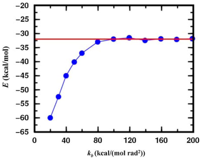
The average of energies of all conformational minima found by MCRSC (blue) as a function of the bond angle force constant k_b. All averages are calculated for twenty independent trajectories started from the crystal structure of a 55-residue protein (α + β fold class; SCOP id: d1div_2) having an α-helix and a small three-stranded β-sheet, and modeled by a previously used coarse-grained knowledge-based energy function (see Section 6.2). The independent degrees of freedom, X_i, that are reduced to model the relative orientation of the α-helix and the central strand of the β-sheet are Shear, Stretch, Stagger, Buckle, Propeller, and Opening (see Fig. 3c). The rigid segments are connected by a loop which accommodates the flexible molten zone with dependent degrees of freedom, X_d, depicted in Figure 3d. The average energy obtained by Loop Torsion Monte Carlo (LTMC) is shown by the red line.

3.3. Conformational optimization in nucleic acids

In Figure 6, we benchmark MCRSC and MCDFC algorithms according to their effectiveness in locating low energy DNA conformations; both the depth of energy minima and the number of Monte Carlo iterations needed to reach them can be used as a measure for performance. The figure shows the three sets of independent degrees of freedom used in this test and marks the location of chain breaks. Figure 6a shows that MCRSC reaches DNA conformations with lower energy than MCDFC. MCDFC works better with rigid body coordinates, which is consistent with earlier studies (Rohs et al., 2005). Figure 6b also shows that MCRSC converges most rapidly. Both tests of MCDFC found new low energy conformational states towards the end of the simulation run.

FIG. 6.

Analyzing energetic relaxation of chain breakage-closure Monte Carlo trajectories started from regular B-DNA conformation. Location of the chain break (dotted line) and the independent degrees of freedom, X_i (marked brown), for the three protocols used. In the first protocol (RSC-10, blue), MCRSC is employed on the closure problem of Figure 2b; the nucleotide conformation is changed by “natural” moves to give 10 independent degrees of freedom. In the second protocol (DFC-13, red), MCDFC is employed on P–O5′ bond closure; the nucleotide conformation is changed by “natural” moves with two additional main chain torsion angles and one additional main chain bond angle to give 13 independent degree of freedom. In the third protocol (DFC-14, green), MCDFC is employed on P–O5′ bond closure; the nucleotide conformations are changed by “physical” moves that include rigid body motion of the base to give 14 independent degrees of freedom. In all protocols, the dependent degrees of freedom, X_d, include torsion angle variables (magenta) that are depicted next to the bond around which the rotation is applied. Unless indicated otherwise, bond angles at all atoms along the chain also contribute to X_d. (a) The averaged value of the total energy as a function of Monte Carlo iterations where the averages are calculated from 10 independent runs. (b) The cumulative variation of the averaged total energy over the final 400,000 Monte Carlo iterations. (c) The distribution of the averaged total energy using the same data as in (b).

3.4. Conformational optimization in proteins

In Figure 7, we benchmark the LTMC and MCRSC algorithms for conformational optimization of protein structures. The figure shows the two sets of independent degrees of freedom used in this test; loop torsion angles and natural coordinates serve as independent degrees of freedom for LTMC and MCRSC, respectively. Figure 7a shows that LTMC and MCRSC trajectories are similar when stiff bond angles are used (k_b2). When softer bond angles are used (k_b1), MCRSC trajectories visit conformational minima with lower energy. Figures 7b shows that the number of MCRSC iterations that leads to convergence does not increase with softer bond angles. Figure 7d shows that MCRSC with soft bond angles not only finds lower energy states but explores the conformational space significantly better in that there are more structures in the low energy values.

FIG. 7.

Energy relaxation of the native structure of a 55-residue protein (α + β fold class; SCOP id: d1div_2) with an α-helix and a three-stranded β-sheet. Each amino acid residue is modeled using three centers: the alpha carbon, the carbonyl oxygen, and a side-chain atom that is closest to the center of mass of the side chain. All pairwise interactions are described by a statistical/knowledge-based energy (see Section 6.2). Simulations are performed using two different Monte Carlo protocols. In the first one, Monte Carlo Recursive Stochastic Closure (MCRSC; blue box on the upper right), six independent rigid-body degrees of freedom, X_i (shown in brown), describe the relative arrangement of the central β-strand and the α-helix. Recursive Stochastic Closure (RSC) works on the molten zone between magenta atoms and sets the value of the dependent variables, X_d (magenta). In the second one, LTMC (red box on the middle right), the relative arrangement of the two segments is described by six independent loop torsion angles (LT). As torsion angle moves in loops move the entire chain, no chain breakages occur. (a) Showing the average value of the knowledge-based energy plotted against the number of Monte Carlo steps for trajectories started at the native conformation and averages are calculated from 10 independent runs. Given that the stochastic closure has bond angle flexibility, MCRSC is used with harmonic potentials to keep all bond angles close to their initial value. MCRSC simulations (blue) were performed using two distinct harmonic constants k_b1 = 40.0 kcal/(mol rad²) and k_b2 = 200.0 kcal/(mol rad²) for stiff and soft bond angles, respectively. The knowledge-based energy (red) as a function of LTMC steps is also plotted. (b) Showing the cumulative average of the expected knowledge-based energy over the 400,000 Monte Carlo iterations. (c) Showing the knowledge based energy distribution calculated using the data in (b). (d) Showing the energy versus RMSD plot for LTMC an MCRSC with soft bond angles.

4. DISCUSSION

4.1. Methods that facilitate natural degrees of freedom in nucleic acids

When comparing MCRSC to MCDFC, an established method that works with natural degrees of freedom in nucleic acids, we found that MCRSC works with chain breaks that are an order of magnitude larger. While its simplicity and low computational cost makes DFC a practical closure method for biological applications, our results show that its use largely depends on the break in the chain being small. We found that RSC is more robust while still maintaining the simplicity and low computational cost of DFC. Our result also indicates that consecutive RSC cycles increase the acceptance rate because they correct the stereochemistry that may not be corrected by the first RSC cycle. Therefore, additional RSC cycles help in that they produce an energetically favorable closure by removing bond and torsion angle strain of the atomic chain spanning the molten zone.

4.2. Robust algorithms for chain closure

Our results indicate that replacing the single atom molten zone used by DFC with the multi-atom molten zone used by RSC enhances robustness in restoring large chain breaks. In general, increasing the number of atoms in the molten zone or equivalently the number of degrees of freedom, N_d, that is used to restore chain breaks enhances the robustness of RSC. In addition, as it was demonstrated in Section 2.2, the computational complexity of RSC is O(N_d). This linear scaling in N_d enabled us to use up to N_d = 2 N_m + 5 = 19 (N_m = 7 was used for proteins) degrees of freedom for chain closure. In contrast, the computational complexity of current multi-atom closure algorithms is O(f_NP(N_d)), where f_NP refers to a non polynomial function. Thus, current algorithms are limited to a value of N_d = 6 and the degrees of freedom include either six torsion angles (Dodd et al., 1993) or three bonds and three torsion angles (Umscneider and Jorgensen, 2003). By defining six constraints, the complicated geometric problem of six equations with six unknowns could have from 2 to 12 numerical solutions (Dodd et al., 1993) with average dihedral angle variations of 40°. Jump between different solutions usually leads to a steric clash between the rigidly attached side chains and surrounding atoms (Hoffmann and Knapp, 1996). In contrast to these algorithms, solutions are iteratively improved by each RSC cycle that builds on and refines the solution found by the preceding cycle.

4.3. Methods that facilitate natural degrees of freedom in proteins

We investigated how MCRSC relates to LTMC which we have shown to efficiently explore protein conformations along natural degrees of freedom in applications including model peptides (Minary and Levitt, 2006) and structures representing all protein folds (Minary and Levitt, 2008). Our finding implies that as bond angles become stiff MCRSC and LTMC sample from the same space of arrangements of secondary structure segments. Our results also indicate that soft bond angles permit more variety in the orientation of structural segments so that MCRSC is able to discover energetically more favorable tertiary arrangements. This finding high-lights some limitations of LTMC that could be overcome by varying bond angles in addition to torsion angles. Unfortunately, this would introduce additional independent degrees of freedom, which would slow down the search of conformational space. By contrast, the independent degrees of freedom of MCRSC are strictly restricted to the orientation of segments. All loop conformations are changed by the dependent degrees of freedom so as to keep the segments connected; this does not slow down the search. When studying larger systems, simple variations in the loop torsional degrees of freedom lead directly to steric clashes that reduce the search efficiency. Again MCRSC is more successful because of local moves that vary the orientation of a segment but leave the rest of the molecule unchanged. Without bond angle variation there is a rough energy landscape that LTMC is unable to explore by simple Monte Carlo protocols as described in Metropolis et al. (1953). None of these limitations are present with MCRSC which explores the smooth loop torsional & bond angle energy surface and samples short and long protein chains with equal efficiency. Note, that the use of natural degrees of freedom for conformational exploration by the popular fragment based algorithms of Simons et al. (1997) is restricted to non-continuous sampling.

4.4. Conformational optimization of proteins and nucleic acids

In our study of conformational relaxation of DNA, we compared the two most cost-effective algorithms, MCRSC and MCDFC. Using the natural degrees of freedom, we found that relaxation driven by MCRSC leads to lower energies and converges faster than relaxation driven by MCDFC. In addition, the distributions of the energy imply that MCDFC gets easily trapped in various conformational basins with diverse energies. The superior performance of MCRSC is partly due to treating some of the independent degrees of freedom of MCDFC as dependent degrees of freedom that are adjusted to further accommodate natural moves. For example, in the present case the three variables are the two torsion angles (γ, ε) and the bond angle at O3′. Treating these variables as dependent in MCRSC not only facilitates natural moves but also improves convergence by reducing the number of independent variables. In accordance with previous studies by Rohs et al. (2005), we found that MCDFC performs well if the global orientation of individual nucleotides is varied by simple translational and rotational moves.

MCRSC was also benchmarked in relaxing the tertiary structure of our protein example. In accordance with our previous findings, MCRSC with stiff bond angles and LTMC relaxed the initial structure with the same efficiency. This implies that in average they converge to very similar conformational states. Removing the stiffness from bond angles opens a passage around torsional energy barriers so that MCRSC could discover new favorable tertiary arrangements. The large variation of their RMSD distance from the initial state implies that the new arrangements are not just energetically refined structures found by LTMC but ones that may represent new fold topologies.

4.5. Limitations of our work

Any conformational modeling study is as good as the force field that is used by the sampling or optimization algorithm. In this article, we focus on the description and testing of a novel algorithm rather than characterizing conformations we generate. While successful biological applications that use our algorithm may rely on a particular force field, testing force fields or reproducing biologically relevant findings is not in the scope of the current article. Benchmarking the performance of alternative multi-atomic closure methods has also not been done in the current study, because either they have not been shown to work with the present type of natural moves, or their computational complexity does not allow the use of a sufficient number of closure degrees of freedom.

Like MCM, MCRSC is designed to sample a transformed energy surface in which some of the transition energy barriers are removed. Thus, both MCM (Li and Scheraga, 1987; Wales and Scheraga, 1999) and MCRSC are not expected to generate canonically distributed conformational ensembles along all degrees of freedom of the original energy surface. Nevertheless, MCRSC may be used as a canonical sampling method along the independent degrees of freedom. Proof of this property is not in the scope of our current work, but it is similar to that used to show that the very successful MCM explores conformational space well.

5. CONCLUSION

This article has presented a novel approach to the chain closure problem. It differs from existing work in that it combines their beneficial features such as simplicity and cost effectiveness, but is more robust and generally applicable. Thus, large chain breaks that are caused by functionally relevant natural moves can still be restored. As a result, the new chain breakage-closure protocol has been demonstrated to explore conformational space more effectively then currently used protocols for both nucleic acids and proteins. Given its capabilities, use of MCRSC is expected to advance our understanding of a large variety of problems in structural biology and macromolecular biochemistry. Such problems include protein and RNA folding, small molecule docking, protein-protein, and protein-nucleic acid interactions and the refinement of experimental structures.

6. MATERIALS

6.1. Nucleic acid structures and models

Initial DNA conformations are obtained from the idealized B-DNA form of the 12 base-pair pappilo-mavirus E2 protein DNA binding site (5′-ACCGAATTCGGT-3′) which has been determined by X-ray crystallography (Hizver et al., 2001). The Cornell et al. (1995) AMBER force field and an implicit electrostatic solvent description by Hingerty et al. (1985) was applied here throughout all energy calculations. The later relatively simple description of the solvent is not only in very good agreement with experimental data but also indispensable here in order to realize the computational advantage of collective moves. More sophisticated implicit solvent models as reviewed in Tsui and Case (2001) would require the costly calculation of the Born radii at each step due to the extensive change in the conformational space. Charges of the DNA backbone are neutralized by the explicit presence of sodium counterions, which rapidly sample the 20 Å cylinder around the DNA. The current model used here has been already extensively tested to reproduce crucial details of all atom explicit solvent simulations performed on the same binding site in Rohs et al. (2005).

6.2. Protein structures and models

The protein studied here has 55 residues and represents one of the α + β fold classes from the SCOP-1.71 database introduced by Murzin et al. (1995). The structure of this particular protein was obtained through the ASTRAL database (Brenner et al., 2000) by following SCOP id: d1div_2. Built on previous work (Minary and Levitt, 2008) the protein was described by a three center per residue knowledge based model. Here, the three centers used for each residue are the C_α atom, the carbonyl oxygen and a single side chain atom used to represent the center of mass of the side chain. Any side chain atom used for a particular residue is taken as the atom that is most commonly closest to the actual center of mass of the side chain in known proteins. In this way the knowledge based energy function derived on atomic positions can be easily adopted. The current coarse grained potential has been extensively tested in Minary and Levitt, (2008) to reproduce near native state features of a large number of folds.

6.3. Monte Carlo move

In all Monte Carlo methods, new conformations are selected from an N dimensional normal distribution, N_N (μ, Σ), where N is the number of independent degrees of freedom of a particular type, the center of normal distribution, μ, is the current state, the uniform standard deviation is Σ_ii = σ_i, = σ; i = 1, …, N and the move size is σ. The unit of measurement for σ depends on the nature of the move: for translational moves σ is in Ångstroms and for rotational moves it is in radians.

6.4. Software

Idealized B-DNA form was generated by the nucgen software package described in Bansal et al. (1995). All methods and algorithms described in this article are implemented in our MOSAICS software package (Minary, 2010), which is available on request from the corresponding author.

7. APPENDIX

7.1. Updating independent degrees of freedom, X_i

We can divide any molecular assembly into N_s arbitrary structural segments, S_k, for k = 1, …, N_s. We chose a center group, C_k, comprising of three atoms in the center of each segment and group, ^SG_k containing the coordinates of all the remaining atoms in S_k. The independent degrees of freedom of the system, which can be internal to a segment or else global, are updated using the following subroutine:

	subroutine update_idof(Xi)
1.	for k ← 1 to Ns do
2.	call resolve (SGk)
3.	iXi ← (update) [iXi]
4.	gXi ← (update) [gXi]
5.	for k ← 1 to Ns do
6.	call rebuild (SGk)

First, the positions of each atom in ^SG_k are resolved into internal coordinates (line 2) using subroutine resolve defined in Section 7.3. Next, all independent coordinates are updated (lines 3 and 4, see Section 6.3). Internal independent degrees of freedom, ⁱX_i may include bend and torsion angles whereas all information about the global independent degrees of freedom, ^gX_i is encoded into the Cartesian position and orientation of each center group, C_i; updating the position and orientation of the center groups effectively updates ^gX_i (line 4; Figure 3a,b). Finally, we calculate the Cartesian coordinates of all segments by subroutine rebuild defined in Section 7.3.

7.2. Setting dependent degrees of freedom, X_d

After all independent variables are updated (see Section 7.1), there may be chain breaks present in the structural assembly. Adjacent to the break we have a molten zone. Following Section 2.2, the atom across the break from the molten zone is known as the “head” atom; the two atoms on the other side of the molten zone are known as the “anchor” atoms. In general, we can assume that there are N_c chain break locations and adjacent molten zones, M_l, l = 1, …, N_c. In ^MG_l, we store coordinates of the molten zone plus the head and anchor atoms associated with M_l. In order to maintain all connectivity (e.g., branching atoms, side chains) when the position of M_l is changed, additional atoms need to be moved. For each M_l, the coordinates of all these atoms are stored in ^BG_l. The execution of one RSC cycle in each molten region is done by the following subroutine.

	subroutine general_rsc(Xd)
1.	for l ← 1 to Nc do
3.	call resolve(BGl)
4.	call rsc(MGl, 1)
5.	call rebuild(BGl)

First atoms in ^BG_l are resolved into internal coordinates (line 3). Next subroutine rsc (see Section 2.2) is executed (line 4) where the recursive iteration is started with the first atom. Finally, all atoms in ^BG_l are rebuilt into Cartesian coordinates (line 5). The loop is going through all molten zones.

7.3. The missing subroutines

Given group G = {r_g(i): i = 1, …, N_g} comprising the coordinates of N_g atoms, transforming all coordinates from Cartesian to internal and from internal to Cartesian variables is done by the following subroutines:

	subroutine resolve (G)
1.	for i ← Ng to 1 do
2.	(b(1), b(2), b(3)) ← (base) [g (i)]
3.	rg(i) ← R(rb(1), rb(2), rb (3)) · (r g(i) − rb(3))
4.	rg(i) ← (rg(i), θg(i), φg(i)) [xg(i), yg(i), zg(i)]

	subroutine rebuild (G)
1.	for i ← 1 to Ng do
2.	rg(i) ← (xg(i), yg(i), zg(i)) [rg(i), θg(i), φg(i)]
3.	(b(1), b(2), b(3)) ← (base) [g (i)]
4.	rg(i) ← rb(3) + RT(rb(1), rb(2), rb(3)) · rg(i)

For each atom function “base” returns the indices of three atoms whose Cartesian coordinates define the local reference frame used to express the atom position in internal variables. Therefore, ordering of atoms from 1 to N_g is done in a way such that the base atoms of an atom are expressed in Cartesian coordinates every time when the atom coordinates are transformed. Note that base atoms that are not in G are always assumed to have Cartesian positions while these transformations are performed. To obtain rotation matrix, R, two unit vectors, e₁ = (r_b(3) − r_b(2))/|r_b(3) − r_b(2)| and e₂ = (r_b(1) − r_b(2))/|r_b(1) − r_b(2)| are first constructed, where |…| denotes Euclidean lengths. Next, e₁ and e₂ are used to construct a local coordinate frame spanned by three vectors, e_z = e₁, e_y = (e₁ × e₂)/|e₁ × e₂| and e_x = (e_y × e_z)/|e_y × e_z|. Given, e_x, e_y and e_z, R = (e_x^T, e_y^T, e_z^T)^T, where e_i^T refers to the transpose of column vector, e_i, i ∈ {x, y, z}.

7.4. The missing proofs

Proof of Lemma 2

Next to each chain break, there is a molten zone, M_l, l = 1, …, N_c. The cost of applying an RSC cycle to M_l is n_l c_spc + c_dfc, where n_l = ^lN_m − 1 and ^lN_m is the number of atoms in M_l. Changing the position of ^lN_m number of atoms will alter ^lN_m + 2 bond angles and ^lN_m + 3 torsion angles. Thus, the number of degrees of freedom used to repair the chain break adjacent to M_l is ^lN_d = 2 ^lN_m + 5. Therefore, n_l = ½ (^lN_d − 5) − 1 and the number of operations used to perform one RSC cycle to each molten zone is Σ_l ((½ (^lN_d − 5) − 1) c_spc + c_dfc) = (½N_d − 3.5 N_c) c_spc + N_c c_dfc where N_d = Σ_l^lN_d is the total number of dependent degrees of freedom changed when applying an RSC cycle to each molten zone. Thus, the asymptotic cost O((½N_d − 3.5 N_c) c_spc + N_c c_dfc) < ½ c_spc O(N_d) + c_dfc O(N_c).

Proof of Lemma 3

Following Lemma 2, the asymptotic cost is ½ c_spc O(N_d) + c_dfc O(N_c). Next, we can make two assumptions: (1) The number of bonds does not exceed the number of atoms in a molecular system, N_c ≤ N. (2) The total number of closure degrees of freedom must always be bonded by the maximum number of degrees of freedom, N_d < 3N. Thus, ½ c_spc O(N_d) + c_dfc O(N_c) < 1.5 c_spc O(N) + c_dfc O(N).

References

- Bansal M, Bhattacharyya D, Ravi B. NUPARM and NUCGEN: software analysis and generation of sequence dependent nucleic acid structures. Bioinformatics. 1995;11:281–287. doi: 10.1093/bioinformatics/11.3.281. [DOI] [PubMed] [Google Scholar]
- Barhen J, Protoposecu V, Resiter D. Trust: a deterministic algorithm for global optimization. Science. 1997;276:1094–1097. [Google Scholar]
- Brenner SE, Koehl P, Levitt M. The ASTRAL compendium for protein structure and sequence analysis. Nucleic Acids Res. 2000;28:254–256. doi: 10.1093/nar/28.1.254. [DOI] [PMC free article] [PubMed] [Google Scholar]
- Brooks CL, Onuchic JN, Wales DJ. Taking a walk on a landscape. Science. 2001;293:612–613. doi: 10.1126/science.1062559. [DOI] [PubMed] [Google Scholar]
- Cornell W, Cieplak P, Bayly C, et al. A second generation force field for the simulation of proteins, nucleic acids and organic molecules. J Am Chem Soc. 1995;117:5179–5197. [Google Scholar]
- Dodd LR, Boone TD, Theodoru DN. A concerted rotation algorithm for atomistic Monte Carlo simulation of polymer melts and glasses. Mol Phys. 1993;78:961–996. [Google Scholar]
- Geyer CJ. Computing science and statistics. Proc 23rd Symp Interface. 1991:156–163. [Google Scholar]
- Gibson KD, Scheraga HA. Minimization of polypeptide energy. I Preliminary structures of bovine pancreatic ribonuclease S-peptide. Proc Natl Acad Sci USA. 1967a;58:420–427. doi: 10.1073/pnas.58.2.420. [DOI] [PMC free article] [PubMed] [Google Scholar]
- Gibson KD, Scheraga HA. Minimization of polypeptide energy. II Preliminary structures of oxytocin, vasopressin, and an octapeptide from ribonuclease. Proc Natl Acad Sci USA. 1967b;58:1317–1323. doi: 10.1073/pnas.58.4.1317. [DOI] [PMC free article] [PubMed] [Google Scholar]
- Hestenes MR, Stiefel E. Methods of conjugate gradients for solving linear systems. J Res Natl Bur Stand. 1952;49:6. [Google Scholar]
- Hingerty B, Richie RH, Ferrel TL. Dielectric effects in biopolymers: the theory of ionic saturation revisited. Biopolymers. 1985;24:427–439. [Google Scholar]
- Hizver J, Rozenberg H, Frolow F, et al. DNA bending by an adenine-thymine tract and its its role in gene regulation. Proc Natl Acad Sci USA. 2001;98:8490–8495. doi: 10.1073/pnas.151247298. [DOI] [PMC free article] [PubMed] [Google Scholar]
- Hoffmann D, Knapp EW. Ploypeptide folding with off lattice Monte Carlo dynamics: the method. Eur Biophys J. 1996;24:387–403. [Google Scholar]
- Kirkpatrick S, Gelatti CD, Vecchi MP. Optimization by simulated annealing. Science. 1983;220:671–680. doi: 10.1126/science.220.4598.671. [DOI] [PubMed] [Google Scholar]
- Krishna P, Theodoru DN. Variable connectivity method for the atomistic Monte Carlo simulation of polydisperse polymer melts. Macromolecules. 1995;28:7224–7234. [Google Scholar]
- Kou SC, Zhou Q, Wong WH. Equi-Energy Sampler with applications in statistical inference and statistical mechanics. Ann Statist. 2006;34:1581–1619. [Google Scholar]
- Levitt M, Lifson S. Refinement of protein conformations using a macromolecular energy minimization procedure. J Mol Biol. 1969;46:269–279. doi: 10.1016/0022-2836(69)90421-5. [DOI] [PubMed] [Google Scholar]
- Li Z, Scheraga HA. Monte Carlo-minimization approach to the multiple-minima problem in protein folding. Proc Natl Acad Sci USA. 1987;84:6611–6615. doi: 10.1073/pnas.84.19.6611. [DOI] [PMC free article] [PubMed] [Google Scholar]
- Metropolis N, Rosenbluth AW, Rosenbluth MN, et al. Estimation of state calculation by fast computing machnies. J Chem Phys. 1953;21:1087–1091. [Google Scholar]
- Minary P, Levitt M. Discussion of the Equi-Energy Sampler. Ann Statist. 2006;34:1638–1641. [Google Scholar]
- Minary P, Levitt M. Probing protein fold space with a simplified model. J Mol Biol. 2008;375:920–933. doi: 10.1016/j.jmb.2007.10.087. [DOI] [PMC free article] [PubMed] [Google Scholar]
- Minary P, Martyna GJ, Tuckerman ME. Algorithms and novel applications based on the isokinetic ensemble. I Biophysical and path integral molecular dynamics. J Chem Phys. 2003;118:2510–2526. [Google Scholar]
- Minary P, Tuckerman ME, Martyna GJ. Long time molecular dynamics for enhanced conformational sampling in biomolecular systems. Phys Rev Lett. 2004;93:150201–150204. doi: 10.1103/PhysRevLett.93.150201. [DOI] [PubMed] [Google Scholar]
- Minary P, Tuckerman ME, Martyna GJ. Dynamical Spatial Warping: a novel method for the conformational sampling of biophysical structure. SIAM J Sci Comput. 2008;30:2055–2083. [Google Scholar]
- Minary P. MOSAICS: Methodologies for Optimization and SAmpling In Conformational Studies. 2010. (in preparation) [Google Scholar]
- Murzin AG, Brenner SE, Hubbard T, et al. SCOP: a structural classification of proteins database for the investigation of sequences and structures. J Mol Biol. 1995;247:536–540. doi: 10.1006/jmbi.1995.0159. [DOI] [PubMed] [Google Scholar]
- Nayeem A, Vila J, Scheraga HA. A comparative study of the simulated-annealing and Monte Carlo with minimization approaches to the minimum energy structures of polypeptides: met-enkephalin. J Comput Chem. 1991;12:594–605. [Google Scholar]
- Rahman JA, Tully JC. Puddle-jumping: aflexible sampling algorithms for rare event systems. Chem Phys. 2002a;285:277–287. [Google Scholar]
- Rahman JA, Tully JC. Puddle-skimming: an efficient sampling of multidimensional configurational space. J Chem Phys. 2002b;116:8750–8760. [Google Scholar]
- Rohs R, Sklenar H, Shakked Z. Structural and energetic origins of sequence specific DNA bending: Monte Carlo simulations of papillomavirus E2 DNA binding sites. Structure. 2005;13:1499–1509. doi: 10.1016/j.str.2005.07.005. [DOI] [PubMed] [Google Scholar]
- Schlick T, Overton M. A powerful truncated Newton method for potential energy minimization. J Comput Chem. 1987;8:1025–1039. [Google Scholar]
- Simons KT, Kooperberg C, Huang E, et al. Assembly of protein tertiary structures from fragments with similar local sequences using simulated annealing and Bayesian scoring functions. J Mol Biol. 1997;268:209–225. doi: 10.1006/jmbi.1997.0959. [DOI] [PubMed] [Google Scholar]
- Sklenar H, Wustner D, Rohs R. Using internal and collective variables in Monte Carlo simulations of nucleic acid structures: chain breakage/closure algorithms and associated Jacobians. J Comput Chem. 2006;27:309–315. doi: 10.1002/jcc.20345. [DOI] [PubMed] [Google Scholar]
- Swedensen RH, Wang JS. Nonuniversal critical dynamics in Monte Carlo simultions. Phys Rev Lett. 1987;58:86–88. doi: 10.1103/PhysRevLett.58.86. [DOI] [PubMed] [Google Scholar]
- Olson WK, Lu XJ. 3DNA: a software package for the analysis, rebuilding and visualization of three dimensional nucleic acid structures. Nucleic Acid Res. 2003;31:5108–5121. doi: 10.1093/nar/gkg680. [DOI] [PMC free article] [PubMed] [Google Scholar]
- Tanner MA, Wong WH. The calculation of posterior distributions by data augmentation. J Am Statist Assoc. 1987;82:528–550. [Google Scholar]
- Tsui V, Case DA. Theory and applications of the generalized Born solvation model in macromolecular simulations. Biopolymers. 2001;56:275–291. doi: 10.1002/1097-0282(2000)56:4<275::AID-BIP10024>3.0.CO;2-E. [DOI] [PubMed] [Google Scholar]
- Umscneider JP, Jorgensen WL. Monte Carlo backbone sampling for polypeptides with variable bond angles and dihedral angles using concerted rotations and Gaussian bias. J Chem Phys. 2003;118:4261–4271. [Google Scholar]
- Voter AF. Hyperdynamics: accelerated molecular dynamics of infrequent evnets. Phys Rev Lett. 1997;78:3908–3911. [Google Scholar]
- Wales DJ, Scheraga HA. Global optimization of clusters, crystals and biomolecules. Science. 1999;285:1368–1372. doi: 10.1126/science.285.5432.1368. [DOI] [PubMed] [Google Scholar]
- Wu MG, Deem MW. Analytical rebridging Monte Carlo: application to cis/trans isomerization in proline containing cyclic peptides. J Chem Phys. 1999;14:6625–6632. [Google Scholar]