Cellular-resolution population imaging reveals robust sparse coding in the Drosophila Mushroom Body

Abstract

Sensory stimuli are represented in the brain by the activity of populations of neurons. In most biological systems, studying population coding is challenging since only a tiny proportion of cells can be recorded simultaneously. Here we used 2-photon imaging to record neural activity in the relatively simple Drosophila mushroom body (MB), an area involved in olfactory learning and memory. Using the highly sensitive calcium indicator, GCaMP3, we simultaneously monitored the activity of >100 MB neurons in vivo (about 5% of the total population). The MB is thought to encode odors in sparse patterns of activity, but the code has yet to be explored either on a population level or with a wide variety of stimuli. We therefore imaged responses to odors chosen to evaluate the robustness of sparse representations. Different odors activated distinct patterns of MB neurons, however we found no evidence for spatial organization of neurons by either response probability or odor tuning within the cell body layer. The degree of sparseness was consistent across a wide range of stimuli, from monomolecular odors to artificial blends and even complex natural smells. Sparseness was mainly invariant across concentrations, largely because of the influence of recent odor experience. Finally, in contrast to sensory processing in other systems, no response features distinguished natural stimuli from monomolecular odors. Our results indicate that the fundamental feature of odor processing in the MB is to create sparse stimulus representations in a format that facilitates arbitrary associations between odor and punishment or reward.

Introduction

A general feature of sensory systems is that dense representations by broadly tuned neurons at the sensory periphery are transformed into sparse representations by narrowly tuned neurons in deeper layers. Specifically, in the olfactory system, Olfactory Receptor Neurons (ORNs) respond to a wide range of different odors (Hallem and Carlson, 2006) and synapse onto Projection Neurons (PNs) of the antennal lobe within structures called glomeruli. At this layer, synaptic and circuit mechanisms produce even broader tuning curves in PNs (Bhandawat et al., 2007) while making responses of different glomerular channels more independent of one another (Olsen et al., 2010). Thus, in the antennal lobe odor identity is represented by a dense code comprised of only about 51 different PN types.

The antennal lobe PNs project to the mushroom body (MB), an area involved in learning and memory, where a major reformatting of information occurs. The MB is composed of roughly 2,000 small neurons known as Kenyon cells (KCs) (Aso et al., 2009). Electrophysiological recordings show that, unlike PNs, individual KCs have highly odor-specific responses and odors are represented by sparse population activity in the MB (Perez-Orive et al., 2002; Broome et al., 2006; Murthy et al., 2008; Turner et al., 2008). Theoretical work suggests sparse representations are useful for accurate information storage (Marr, 1969; Kanerva, 1988; Olshausen and Field, 2004) and appear to be a general feature of deeper brain areas.

Broad sampling of population activity is important to thoroughly characterize sparse representations, and to establish that they are truly sparse. Recent advances have dramatically increased the sensitivity of genetically encoded calcium indicators (Tian et al., 2009). Here we use two-photon imaging with the GCaMP3 reporter to simultaneously monitor more than 100 KCs (about 5% of the total) with sensitivity approaching that of electrophysiology.

If sparse coding is truly a fundamental aspect of processing in the MB, it should be robust across a range of different stimulus features. There are two broad challenges to maintaining a sparse representation: variations in stimulus intensity and variations in stimulus complexity. We found that population sparseness was largely robust to increases in odor concentration. To examine the effects of stimulus complexity, we tested responses to both natural and artificial multimolecular odors and compared them to monomolecular compounds. We observed similar levels of sparseness across all stimulus categories, even complex natural stimuli. Interestingly, there were no response features that distinguished representation of monomolecular and natural odors. This contrasts with other sensory systems where there are substantial differences in the coding of natural and artificial stimuli (Rieke et al., 1995; Machens et al., 2001; Yu et al., 2005; Garcia-Lazaro et al., 2006). Finally, we found no obvious spatial arrangement of KC somata based on odor tuning properties or responsiveness.

In contrast to other sensory systems, where familiar or behaviorally meaningful stimuli appear to be represented distinctively, the MB represents all stimuli sparsely, and responsive cells are randomly organized. This is similar to piriform cortex (Stettler and Axel, 2009), and likely reflects the role of both these brain areas in learning arbitrary associations between odor and reward or punishment.

Materials and Methods

Fly Stocks

Flies were reared on standard medium, supplemented with dry baker’s yeast (Saf-Instant, Lesaffre Yeast Corporation), at room temperature (22-25°C). Flies carrying the genetically encoded calcium sensor UAS-GCaMP3 (Tian et al., 2009) were crossed with OK107-Gal4 (Connolly et al., 1996), to drive GCaMP3 expression in essentially all KCs (Lee et al., 1999; Aso et al., 2009). All experiments were conducted on female F1 heterozygotes from this cross, aged 2-5 days post-eclosion. GCaMP expression has not been observed to affect normal neuronal function in Drosophila (Jayaraman and Laurent, 2007).

Animal Preparation

Procedures for animal preparation were based on earlier methods (Turner et al., 2008; Murthy and Turner, 2010). Briefly, flies were transferred to a glass tube and anesthetized on ice until movement ceased (about 15 s). A female fly was then gently inserted into a rectangular hole (about 0.77 by 1.5 mm) cut into a piece of aluminum foil glued to the underside of the recording platform. The fly’s head was tilted forward to provide access to the posterior surface of the brain where the KC cell bodies are located. The olfactory organs point downwards in this preparation, allowing airborne odor delivery (Figure 1A). The fly was fixed in place using fast-drying epoxy (Devcon 5-Minute Epoxy).

Figure 1.

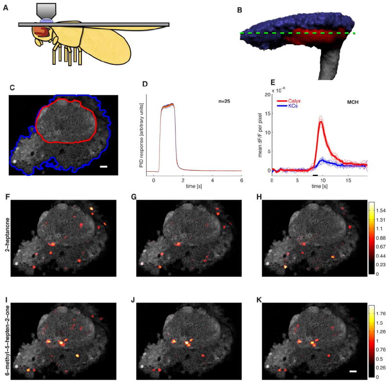
Odors evoke consistent patterns of calcium activity in the mushroom body. A. Schematic of a fly in the recording platform. Mushroom body is shown in dark gray behind the fly’s eye. B. Three dimensional reconstruction of the mushroom body (MB) obtained using the OK107-Gal4 driver. The Kenyon cell (KC) somatic region is shown in blue, the input neuropil region (calyx) in red, and axonal outputs in gray. The green dashed line indicates a typical imaging plane. C. Optical section through the MB showing the clearly distinguishable KC somatic region (blue) and dendrites in the calyx (red). Image is obtained by averaging 12 frames of basal GCaMP3 fluorescence. D. Timecourses of 25 pulses of isoamyl acetate measured using a photo-ionization detector (PID; arbitrary units) showing the high reliability of odor delivery. Odor delivery valve opens at t = 0 s and closes at t = 1 s. PID data are smoothed with a 0.1s boxcar filter. E. Mean change in fluorescence per pixel following presentation of 4-methylcyclohexanol (black bar) in the calyx (red) and KC region (blue) from the optical section shown in C. Thin lines show 5 individual odor presentation trials and thicker lines the means. The dF/F values are low because most pixels do not change in intensity. F-K. Basal fluorescence (gray) and mean evoked dF/F (heat map) from the experiment shown in C. Mean dF/F is calculated over 0.5 to 4.5 s following stimulus onset. Each row shows responses to three different presentations of the same odor. Responses are evident both in the dendritic region in the calyx (red outline in C) and the cell body area (blue outline in C). The pattern of responding neurons is similar within an odor and different across odors. Scale bars indicate 10 μm.

The bath surrounding the head capsule was continuously perfused with oxygenated saline (Wilson et al., 2004) and the cuticle at the back of the head was dissected away using sharpened forceps. We sometimes found it necessary to minimize brain motion by removing the pulsatile organ at the neck (care was taken to avoid damaging the gut) and the proboscis retractor muscles, which pass over the caudal aspect of the optic lobes. Air sacs and fat deposits occluding the MB were cleared from the brain’s surface. We did not purposefully attempt to remove the peri-neural sheath, as is needed for electrophysiological experiments. Flies remained healthy and active throughout the experiment, as evidenced by abundant voluntary leg movements. Many preparations were discarded due to excessive brain motion that prevented us from tracking individual neurons throughout the imaging session.

Odor Stimuli

The following chemicals were used as stimuli: 2-heptanone (CAS No. 110-43-0), 3- octanol (589-98-0), 6-methyl-5-hepten-2-one (110-93-0), α-humulene (6753-98-6), benzaldehyde (100-52-7), ethyl lactate (97-64-3), ethyl octanoate (106-32-1), hexanal (66-25-1), isoamyl acetate (123-92-2), 4-methylcyclohexanol (589-91-3), methyl octanoate (111-11-5), diethyl succinate (123-25-1), pentanal (110-62-3), and pentyl acetate (628-63-7). In addition to these monomolecular odorants, apple cider vinegar (Richfoods), and reconstituted dry baker’s yeast (Saf-Instant, Lesaffre Yeast Corporation) were used. Fresh fruits (banana, mango, and orange) were obtained from a local grocer.

Odor Delivery

We built a 12-channel odor delivery system capable of air-diluting pure odorants up to 1×10^-4. Odor stimuli were kept in 40 mL sample vials each containing 3-4 mL of odorant and a strip of filter paper to aid evaporation and maintain a saturated headspace concentration. Using a smaller volume of odorant tended to produce inconsistent stimulus delivery, as measured with a photo-ionization detector (PID, Aurora Scientific). The delivery system required accurate airflow, which was achieved using fast mass flow controllers and meters (Alicat Scientific). In most experiments, saturated vapor from pure odorant was serially diluted in air to achieve a dilution ratio of 1:100. For the odor mixture experiments (Figure 7), headspace from separate vials containing monomolecular odors was combined, so the concentration of each component in the mixture was the same as the components presented individually. Headspace from vials containing orange, mango, yeast, and apple cider vinegar was presented at 1:2 dilution.

Figure 7.

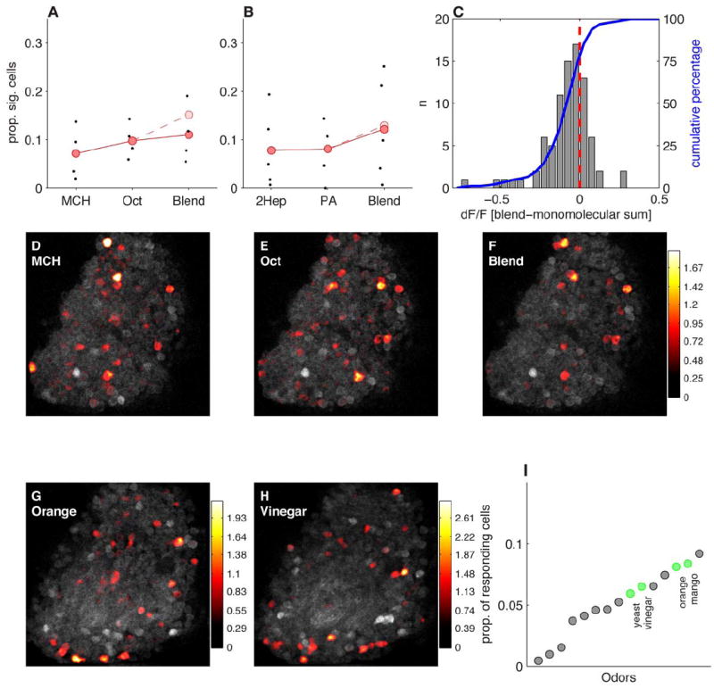
MB responds sparsely to complex and natural odorants. A. Proportion of KCs responding to 4-methylcyclohexanol (MCH), 3-octanol (Oct), and a 50:50 blend of the two odorants. Points show sparseness values from individual optical sections (n=4). Grand means shown in red. The sparseness of responses to the blend is very similar to that of the monomolecular components. The pale red point indicates expected proportion of responsive cells if the monomolecular odorants were to sum additively. B. Similar data as A, but from a different experiment using 2-heptanone, pentyl-acetate, and their 50:50 blend. C. Responses to blends are predominantly sub-additive. Histogram shows the distribution of deviations from linearity for responses to the Oct+MCH blend compared to the response predicted by linear addition of responses to the individual components. 73% of cells responded less to the blend than expected from the sum of the component responses, indicating that the majority of KC responses to the blend are sub-additive. D-F. Basal fluorescence (gray) and dF/F overlay (heat-map) for responses to 3-octanol, 4-methylcyclohexanol, and the blend of the two odors. Each panel shows data from an individual trial. dF/F values are on the same scale for all panels. G-H. Single-trial responses to two complex natural odors. I. The sparseness values of natural odors (green) compared to a range of different monomolecular odorants (gray). Natural odorants do not evoke responses that are substantially more or less sparse than monomolecular odorants.

Airflow into each vial was regulated by a 2-way inert isolation valve (N-Research #T360K012). Outflow was gated by a zero-dead-volume 4-way inert isolation valve manifold (N-Research #360T082). The manifold consists of a non-gated carrier (clean air) path into which 4 isolation valves connect. Thus, 4 odor vials can be connected to each manifold. Three manifolds were connected in series to allow up to 12 different odors to be used in a single experiment. A separate empty (control) vial was located upstream via two normally-open isolation valves. To present an odor, a small quantity of odorized headspace was injected into the carrier path by closing the control vial valves and simultaneously opening the two valves gating one of the odor vials. We did not use check-valves at any point, as experience showed these to work poorly.

The total airflow coming out of the valve manifolds was always 1 L/min, so the first air dilution was controlled by varying the ratio of airflow between the carrier path and odor vial. This could be optionally diluted further by discarding a known proportion of the flow to vacuum via a needle valve using the principle of choked flow. The remaining odorized stream could then be further diluted by injecting it into a second carrier of up to 5 L/min. The total flow at the fly was regulated using vacuum and a second needle valve. Total airflow over the fly was 1 L/min, except for natural odor experiments, which used a 0.5 L/min flow rate.

A relatively square odor pulse (Figure 1D) was created by switching between clean and odorized air streams using a synchronous 2-way valve (N-Research #648T042SH). This final valve was located about 50 cm from the fly, leading to a delay of about 300 ms between valve switching and odor reaching the fly. Inert tubing (Tygon SE-200) was used for all connections. The flow path was 1/8" internal diameter throughout. This diameter is sufficiently large to allow the system to work near to atmospheric pressure at our flow rates. This virtually eliminated pressure transients caused by valve switching, as measured by an anemometer (Kurz Instruments). The system terminated at a Teflon odor delivery nozzle (1/8" OD, 1/16" ID), beveled so that its tip surrounded the fly’s head. A suction tube was positioned opposite the odor tube to evacuate odorized air.

We monitored odor delivery on every trial using a PID. The flow path was split after the final valve, with half the stream delivered to the fly and half to the PID. The PID response was digitized at 1kHz, and boxcar filtered at 0.1 s.

Calcium Imaging

All 2-photon imaging was done using a Prairie Ultima system (Prairie Technologies) and a Chameleon Ti-Sapphire laser (Chameleon XR, Coherent Inc.) tuned to 920 nm. Beam strength was attenuated with a Pockels cell (Conoptics Inc.) to deliver approximately 8-10 mW at the sample. All images were acquired with Olympus water immersion objectives (LUMPlanFl/IR, 60X, numerical aperture (NA), 0.9 and LUMPlanFl/IR, 40X, NA, 0.8). Emission fluorescence was bandpass filtered using an HQ525/70m-2p filter (Chroma Technologies). Imaging frames varied slightly for each experiment, but were generally around 300×300 pixels, with a pixel dwell time of 1.6 μs, yielding frame rates of roughly 3.8 Hz.

Experimental Protocol

Data were acquired using PrairieView software (Prairie Technologies). Custom MATLAB (The MathWorks) routines were used to control odor presentation and synchronize stimulus delivery with data acquisition. Data were acquired in 25 s sweeps with a 1 s odor pulse triggered 8 s following sweep onset. There was no delay between sweeps so the inter-stimulus interval (ISI) was 25 s. Stimuli were presented in randomized odor blocks. The same odor was never presented twice in succession. The exception to this was the experiment displayed in Figure 6, which was designed to test the effects of presentation order, as discussed in the Results section. Imaging sessions were generally limited to about 20 minutes (i.e. about 48 stimulus presentations with a 25 s ISI) due to gradual changes in brain shape and photobleaching.

Figure 6.

The effects of odor concentration and recent stimulus history on MB population sparseness. A. Stimuli were delivered in blocks of either increasing of decreasing concentration steps, shown here as the average PID traces acquired during each type of experiment (see Results for details). B. Proportion of Kenyon cells responding to ripe banana over a range of different odor concentrations. Mean sparseness increases slightly with concentration, but never exceeds 0.2. Each point is the MB response from an individual fly for each concentration from both types of stimulus blocks (jittered along the x-axis for clarity); dark bars indicate the mean of these points. Light boxes indicate standard deviation around the mean and dark boxes indicate the 95% confidence interval. C. Same as B, but for the monomolecular odor isoamyl acetate. D. Data from B and C showing specifically the results from the high-to-low concentration steps. E. As D, but the low-to-high steps. An effect of concentration is only apparent for the high-to-low condition. F-G. Responses on individual trials over the course of an experiment showing that the order in which stimuli were presented affects the sparseness of MB response. Response to the first trial was typically less sparse than subsequent trials. Additionally, the stimulus block type (high-to-low vs. low-to-high) affected how sparseness changed with concentration. Gray lines show sparseness estimates from individual flies. Points connected by the black line indicate the mean responses on individual trials of different odorant concentrations (filled circles) or clean air (open circles). Trial blocks have been separated in time for clarity, but experiments were run continuously.

Data Analysis

All data analyses were conducted in MATLAB and R (http://www.R-project.org). To correct for motion artifacts, we aligned frames using a sub-pixel translational-based discrete Fourier analysis (Guizar-Sicairos et al., 2008). A region of interest (ROI) was drawn automatically around fluorescent neural tissue. The area outside the ROI was considered to be background fluorescence (auto-fluorescence plus shot noise) and its mean was subtracted from the overall image. To quantify the response of the KCs we applied a small region of interest (ROI), 6 to 8 pixels in diameter, to each cell body. This allows us to average pixels from each cell and treat them as a unit. ROI selection was done manually as somata were packed closely together and of such low contrast that all automated algorithms we tried performed very poorly and required excessive supervision. In each optical section we selected as many KCs as possible. Data were first motion-corrected and aligned using a rigid transform so that all frames across all trials were in register. For each trial we averaged all frames to yield a single mean image. If an experiment consisted of, say, 50 trials then we ended up with 50 of these mean images. KCs were selected by identifying cells from a short looping movie built from the trial-averaged frames. This ensured that each selected cell remained within its ROI over the whole imaging session. Cells which moved excessively, whether responsive or not, were discarded from the dataset.

We used a simple statistical test to determine whether a KC responded significantly on a given trial. We first calculated the standard deviation (SD) of the baseline activity 8 seconds prior to stimulus onset. The response timecourse was then smoothed using a 5-point running average and the peak dF/F in the 0.5 s to 4.5 s window following stimulus onset was determined. The response was judged to be significant if the peak was 2.33 SDs greater than the baseline; this corresponds to a one-tailed significance test where α = 0.01. This is discussed further in the Results. For a KC to be classified as responsive to a given odor, it had to exhibit significant responses to at least half the presentations of that odor. A previous electrophysiological study of KC responses used the same reliability criterion (Turner et al., 2008).

Results

Optical monitoring of MB population activity

To characterize the response of the MB population to a range of different olfactory stimuli, we used two-photon calcium imaging with the genetically encoded calcium indicator GCaMP3 (Tian et al., 2009). We targeted GCaMP3 expression to the MB using the GAL4 driver, OK107, which expresses in all KCs (Lee et al., 1999). We oriented the preparation so that the KC somata are superficial and the imaging axis is perpendicular to the disc-shaped field of cell bodies, maximizing the number of neurons that can be imaged simultaneously (Figure 1A). A typical imaging plane captures roughly 100 of the 2000 total KCs in the MB; the location of the optical section varied across preparations, capturing a different set of KCs in each fly. Slightly deeper optical sections enabled us to image both cell bodies and the dendritic sites in the calyx (Figure 1B-C).

We presented odor stimuli using a custom-built device that could deliver up to 12 different odors in one session. Different odors were delivered in pseudo-randomized order, with a 25 sec inter-stimulus interval (see Methods). Odor delivery was controlled by a series of valves triggered to open for 1 sec, starting 8 sec after trial onset. The actual timecourse and amplitude of odor delivery was directly monitored by splitting the odor flow line so half was delivered to the fly and half to a photo-ionization detector (PID; see Methods). Odor delivery was highly reliable across multiple presentations as measured by PID (Figure 1D), although there was a consistent delay of about 300 ms between valve opening and the onset of the PID signal.

We could detect strong, reliable odor-evoked signals in both the dendritic and somatic region of the MB. Figure 1E shows the proportional change in fluorescence (dF/F) spatially averaged across the calyx (red) and cell body region (blue). The timecourse of the GCaMP3 signal generally lasted for several seconds after odor offset. The amplitude of the calyx signal was much greater than that observed at the cell bodies, which is consistent with calyx signals representing strong synaptic input from PNs, and cell bodies the sparse spiking output.

Responses were generally prolonged (Figure 1E), so we quantified response amplitudes by averaging activity at each pixel from 0.5 to 4.5 seconds following stimulus onset. The bottom two rows in Figure 1(F-K) show the mean evoked odor response (heat-map colors) superimposed on the basal fluorescence (gray scale) from a single fly. The top row shows three responses to 2-heptanone and the bottom row responses to the related compound, 6-methyl-5-hepten-2-one. Presentations of these odors were randomly interleaved with others (data not shown). Activity can be seen in both the cell body region and the calyx (refer to Fig. 1C). Importantly, in the cell body region there are focal, circular, signals visibly attributable to individual KC somata. Note that the same odor activates similar patterns of MB activity across presentations, and response patterns are different between odors.

Determining population responses from somatic calcium signals

The strong baseline fluorescence, together with the high signal-to-noise ratio of the somatic responses made it possible for us to analyze the data at the level of individual cells. This allowed us to evaluate sparseness of representations by directly visualizing the fraction of cells in the imaging plane that respond to a given odor. A cell was deemed to be responsive to an odor based upon two criteria: the presence of a significant dF/F deflection from baseline after odor onset, and the reliability of this deflection across multiple presentations. To be deemed significant, the fluorescence change on a given trial had to exceed 2.33 SD of the dF/F fluctuations observed during the baseline period on that trial. This corresponds to a threshold crossing measure with α = 0.01. To account for trial-by-trial variability we required that this threshold be crossed on more than half of all presentations of an odor. These are similar criteria to those used in previous electrophysiology studies (Turner et al., 2008) and account for the fact that some KCs respond unreliably or weakly, a feature that can accompany sparse representations (Willmore, 2001), and may place a limit on the information carried by the KC population.

These statistical criteria effectively captured the features of the population response that were apparent from visual inspection. Figure 2A shows the timecourse of fluorescence changes for 121 KCs in response to a single presentation of isoamyl acetate. The cells in Figure 2A are sorted by the p-value for the significance of threshold crossing; the 24 cells below the dashed white line exceeded the threshold. Timecourses from cells crossing the threshold are shown in Figure 2B, while those failing to cross are shown in Figure 2C. Panels in Figure 2D-F show dF/F timecourses in response to the control stimulus, an empty vial. Pooling data over the entire experiment makes the distinction between responding and non-responding cells clearer still. We recorded the responses of 121 KCs to 5 odors presented 5 times each, which yielded a total of 3,025 KC-stimulus pairs. The distribution of threshold crossing p-values for these data are shown in the cumulative histogram in Figure 2G. The plot shows a clear elbow due to the presence of a small number of significant trials against a background of non-significant trials. The threshold of α = 0.01 falls at this elbow, indicating that this threshold partitions the data naturally.

Figure 2.

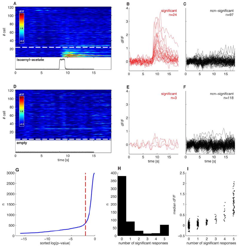
Detecting odor responses with cellular resolution in single trials. A. dF/F timecourses of 121 KCs in response to the presentation of isoamyl acetate (PID trace in gray). KCs are sorted according to the p-value of the threshold crossing (see Results). Cells below the dashed white line show a significant response peak at p < 0.01. B. Timecourses of the 24 significantly responding cells from A. C. Timecourses of the 97 non-responding cells from A. D-F. Responses of the same 121 cells to one presentation of clean air. G. Cumulative histogram of p-values from all cells and all odor presentation trials from a single fly. The α = 0.01 (dashed red line) threshold falls at the elbow of the line indicating that it represents a reasonable distinction between responding and non-responding KCs. H. Histogram showing the number of trials in which each cell exhibited a significant response to an odor; data from 121 KCs presented with 5 different odors (605 KC-odor pairs) for 5 trials each. Data are bimodally distributed, with some cells responding to only one or two of the five total odor presentations. I. Relationship of response amplitude to response reliability from KC-odor pairs shown in H. Cells exhibiting a larger evoked dF/F also showed more reliable responses. Points are jittered along the x-axis for visibility.

To estimate the fraction of KCs that respond to an odor, we also factored in the reliability of those threshold crossings over multiple odor presentations. On any given odor trial, about 20% of KCs may be active (Figure 2A-C). However, only a portion of these cells display significant fluorescence changes on more than two presentations of that odor (Figure 2H). Moreover, we found that cells which respond significantly on more than half of trials are those with the larger median odor-evoked dF/F (Figure 2I), indicating that cells with larger response amplitudes also respond more reliably. Based on these observations, we considered a cell to be responsive to a particular odor if it passed the significance test on more than half of all presentations of that odor. The results obtained from applying our response criteria are shown in Figure 3. Figure 3A-B show the dF/F timecourses and response amplitudes of a cell we classified as responding significantly to 3-octanol but not to clean air. Response amplitudes were calculated as the mean evoked dF/F within the response window (0.5 to 4.5 sec after odor onset). The response amplitudes of 45 cells are shown in Figure 3C, colored according to their classification as responding or non-responding. Responding neurons generally displayed larger dF/F values than non-responding cells, although occasionally their dF/F values were similar. Non-responsive cells were classified as such either because those dF/F changes were not significantly greater than baseline fluctuations, or because they were not reliable across presentations. This is evident in Figure 3D, which shows that the p-values for threshold crossing are invariably smaller over multiple trials for the gray, non-responsive cells.

Figure 3.

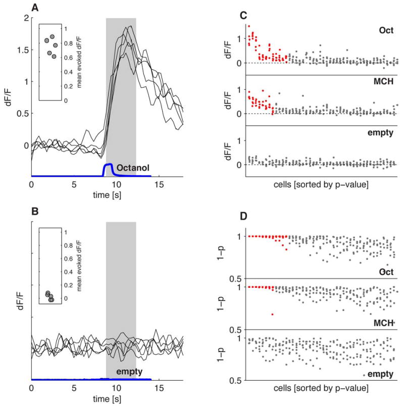
Reliably identifying KC odor responses. A. Responses of a single KC to 5 presentations of 3-octanol (black traces). The blue trace shows the kinetics of the odor pulse measured by PID. Response amplitudes (inset) are calculated by averaging activity between 0.5 and 4.5 seconds following stimulus onset (shaded gray region). B. Responses of the same cell to the clean air control. C. Response amplitudes of the 45 strongest responding neurons from a single optical section to 3-octanol (Oct), 4-methylcyclohexanol (MCH), and clean air. Each data point is the evoked response amplitude from a single cell on a single trial. A cell is deemed responsive to the odor if it responded significantly (p < 0.01) on more than half of trials. Responsive cells are indicated by the red points, non-responsive cells in gray. Cells are sorted independently for each stimulus according to the mean p-value. D. Statistical significance of response peaks from the neurons shown in C. The y-axis shows 1 minus the p-value. Cells are sorted as in C. Note that responsive cells consistently have values close to 1 on almost all trials; this is not the case for cells classified as non-responsive.

To summarize, in order to qualify as responsive to a particular odor, a cell had to exhibit a peak dF/F value that was 2.33 SD (α = 0.01) greater than the baseline mean within a window 0.5 to 4.5 sec after odor onset, on at least half of odor presentations. Both the threshold crossing and reliability criteria were chosen based on features that were evident in the underlying data (Figure 2G-H). The fraction of responding KCs we detect with this method is extremely similar to that observed in previous electrophysiological studies (see below, Turner et al., 2008), suggesting that we detect the vast majority of KC responses. Overall, these results show that we can reliably track activity of individual KCs on a trial-by-trial basis, enabling us to identify consistent KC responses within a large population of cells, and generate an accurate measure of population sparseness.

Random spatial distribution of MB odor responses

We examined whether there was any relationship between the response properties of KCs and their spatial distribution within the cell body layer. Imaging can readily reveal whether there are clusters of cells that represent odors densely, or groups of cells with similar response properties. We tested this by imaging responses to a panel of chemically diverse odors (a total of 18 different odors, 4 to 7 odors per fly). We found that most KCs did not respond to any of the tested stimuli (Figure 4A), as observed previously with electrophysiological recordings (Perez-Orive et al., 2002; Turner et al., 2008). This skewed distribution could reflect a spatial organization consisting of small clusters of densely responding neurons.

Figure 4.

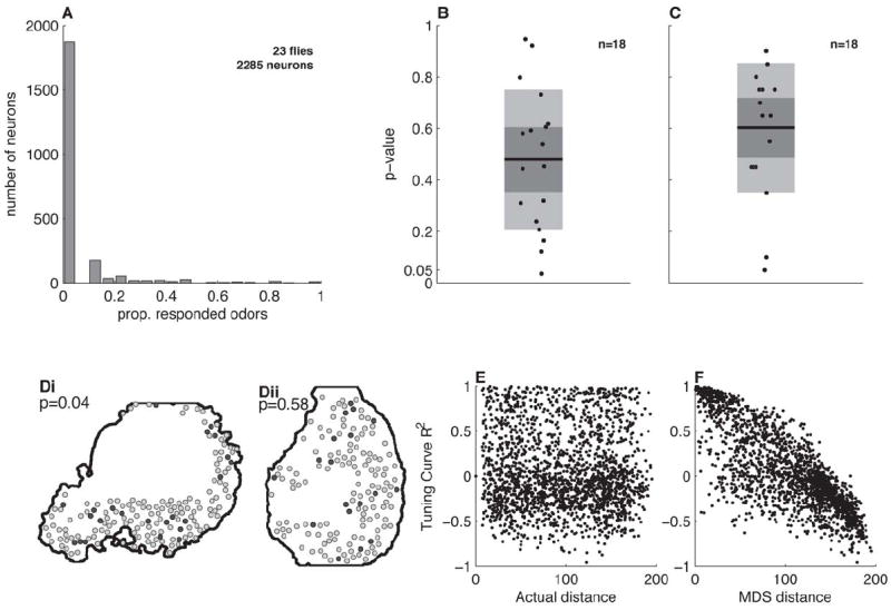
Random spatial distribution of responding MB neurons in the cell body layer. A. The proportion of odors eliciting a response from each cell (lifetime sparseness). The vast majority of cells do not respond to any tested odor (peak at zero). B. Distribution of p-values from a permutation test for clustering of responsive neurons within an optical section. Each data point represents one optical section from an individual fly. Light box indicates standard deviation around the mean and dark box indicates the 95% confidence interval. Only a single imaging plane showed a nominally significant level of clustering (p=0.04). See Results for details. C. Distribution of p-values from a permutation test for clustering of neurons with similar tuning curves. Each data point represents one optical section from an individual fly. We found no evidence for clustering. D. Example imaging planes showing distributions of responsive cells (dark gray). Neither a section with the high clustering value we observed (Di) nor one with a moderate value (Dii) showed a visibly striking clustering of responsive neurons. E. Tuning curve correlation as a function of distance between cells from a single fly. F. Tuning curve correlation as a function of distance in MDS space (see Results) for the fly shown in E. This plot illustrates that obtaining topography is possible with the tuning curves we observe experimentally.

We investigated this possibility by measuring the distances separating responding neurons, and comparing them to the distances expected if these neurons were distributed randomly. Since each experiment involved optical sections from different locations and orientations in the MB, we analyzed each imaging plane individually. We began by identifying cells that responded to at least one odor (preparations with fewer than 10 responding cells were excluded). We then calculated the distance from each responding cell to its nearest responding neighbor. For instance, an imaging field containing 16 responding cells would yield 16 distance values. We calculated the mean of these distances as a measure of clustering; a smaller value indicates tighter clustering. Using nearest-responding-neighbor distances ensured that our analysis would not overlook the possibility of multiple small clusters. We tested the significance of this value using a permutation test where the labels of all identified KCs were randomly reassigned, such that responding cells become located in new, randomly chosen, positions. We recalculated the nearest-responding-neighbor distances and took the mean of these to represent the value expected in the absence of clustering. This procedure was repeated 10,000 times for each fly. If the experimentally observed clustering value was smaller than 95% of the simulated values we considered this to be evidence of significant clustering at α = 0.05 for this particular fly. Figure 4B shows the distribution of p-values from this response clustering test for 18 flies. Overall, these results show no strong evidence for clustering of responsive neurons in the cell body layer, although one fly did have a p-value below the significance level (p = 0.04). The actual distribution of responding neurons in this section is shown in Figure 4Di, where it is apparent that the clustering is not striking. We note that electrophysiological studies have shown that KCs with axonal projections to the α’β’ lobes tend to be more responsive than other KC types (Turner et al., 2008). However our results indicate that this spatial organization is not present in the cell body layer.

It is also possible that KCs are topographically organized according to their odor tuning curves. Here we test the simplest hypothesis: that nearby neurons have tuning curves that are more similar to one another than those of more distant neurons. Tuning curves were calculated as the mean dF/F response evoked by each odor, and tuning curve similarity was measured as the Pearson’s correlation coefficient between each pair of odor tuning curves. We then tested whether there was a relationship between tuning curve similarity and the Euclidean distance between cells using Spearman’s ρ, which evaluates whether there is a monotonic relationship between these two variables. Spearman’s ρ, values were calculated for each imaging plane and, as before, we judged significance using a permutation test. We randomized the identity of the responding cells within the image plane to produce a new Euclidean distance matrix while keeping the tuning curve correlation matrix fixed, and recalculated Spearman’s ρ. This process was repeated 10,000 times to generate a distribution of ρ values expected if tuning curve topography were absent. If the experimentally observed ρ was greater than 95% of the simulated values, we consider there to be significant tuning curve topography in that optical section at the α = 0.05 significance level. Figure 4C shows the distribution of p-values for the test of tuning curve clustering for the 18 flies. All points lie above the significance threshold, indicating that there is no strong tendency for KCs with similar odor tuning to be located near one another.

The odor tuning properties of KCs are extremely diverse, so it may not even be possible to arrange odor tuning curves topographically in 2-D. Therefore, to validate the results above, we confirmed that it was feasible to arrange the tuning curves we measured experimentally in a way that produces a topographic map. To generate an artificial topographic map with the data collected, we arranged KCs in a 2-D space based on the correlations between different tuning curves. Specifically, we projected the correlation matrix into a 2-D space that mimics the imaging plane. We achieved this using multidimensional scaling (MDS), a re-mapping technique which measures the distances between points in a high-dimensional space and projects this onto a low dimensional space (typically 2-D) while attempting to retain the relationship between points (Martinez and Martinez, 2005). We tested whether our regression analysis would reveal topography in the tuning curves arranged in 2-D MDS space. Again, we calculated the corresponding ρ value and compared this to a distribution of 10,000 ρ values generated using randomized Euclidean distance matrices. This analysis showed that the tuning curves we measured could indeed be arranged topographically. In every imaging experiment analyzed (n = 18), the MDS-based topographic map had a greater ρ value than all of the randomized tuning curve maps. Therefore our inability to find topography in the original data was not due to the fact that tuning curve shapes are too varied, or too uncorrelated to be regularly arranged in 2-D.

Together, these results demonstrate that neither do odor representations in the MB cluster spatially, nor do KCs with similar odor tuning properties have apparent spatial localization. This suggests that the relationship between response properties of KCs and their spatial distribution within the cell body layer is random. Such a lack of spatial organization is a shared feature of both the MB and mammalian piriform cortex (Stettler and Axel, 2009), and highlights their likely role as associative areas where anatomical specialization plays a minimal role in information processing.

MB population responses to odors are sparse and correlated with ORN output

Using GCaMP3 we routinely obtained response amplitudes with dF/F values 2 or 3 times greater than the baseline (for example, see Figures 1 and 2). This signal strength is 4 to 6 times higher than that obtained in a previous MB study using GCaMP1.3 (Wang et al., 2004), and suggests that this indicator has the sensitivity to detect most KC activity. Across the range of monomolecular odors shown in Figure 5A, we found that on average an odor evokes responses in about 5% of the KCs in an imaging plane (n = 8 flies and n = 933 neurons); given the lack of spatial clustering of responses, this likely reflects the overall probability of response across the entire MB. This is extremely similar to results obtained using single cell recordings, where on average each odor activates 6% of cells (Turner et al., 2008). The mean proportion of responding cells did not exceed 0.1 for any odor, although the response from individual flies reached values up to 0.17. However, even the largest of these values is well below that observed in PNs, where a given odor often evokes a response in excess of 50% of the population (Wilson et al., 2004). Thus, although we do not exclude the possibility that some KC responses go undetected with GCaMP3, when expressed using the OK107 driver, this indicator clearly enables us to detect KC responses with a level of sensitivity comparable to that of electrophysiology.

Figure 5.

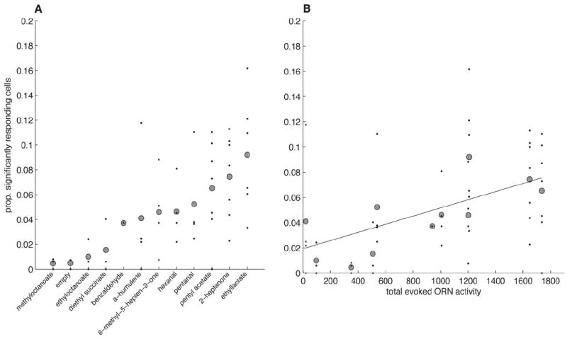
Responses to monomolecular odors are sparse in MB. A. Proportion of KCs responding to a variety of different odors. Black points show sparseness values from individual animals (n=8 flies), gray circles show the grand mean. B. Mean sparseness values as a function of total ORN activity (ORN data from (Hallem and Carlson, 2006)) for each odor. Some KC responses shown in A are not plotted since ORN data do not exist for these odors. The slope of the fit is significantly different from zero (p = 0.0001, see Results).

Is it possible to predict the sparseness of an odor representation in MB? Although there was quite a high level of variability across individual flies, there was still a clear trend for certain odors to evoke a more extensive response in the MB than others. This suggested that sparseness levels could perhaps be predicted by some aspect of the stimulus. One such predictor could be the total activity of olfactory receptor neurons (ORNs) at the sensory periphery. To test this, we examined odorants for which the response properties of 24 adult ORN types are known (Hallem and Carlson, 2006). We used linear regression to predict the proportion of responsive KCs as a function of the total evoked ORN activity (Figure 5B). Since the data included repeated observations from the same fly, we used a mixed-effects linear model (Pinheiro and Bates, 2000) to fit a random intercept for each animal. The slope of the model was significant (p = 0.0001, df = 38) and indicated that, on average, increasing the total ORN activity by 10 spikes/s caused the proportion of responsive KCs to increase by 0.03%. In other words, it would take 16 additional spikes at the ORN level to recruit one additional KC response within the entire MB population. However, the regression explained only about 27% of the variance. There are several possible reasons why this correlation is weak. One is that our prediction is based on the activity of only half the complement of ORNs. A second is that processing by local neurons provides gain control within the antennal lobe, producing similar PN output levels for different intensities of ORN input (Olsen and Wilson, 2008; Root et al., 2008). However, the fact that we find a significant correlation indicates that the gain control mechanisms are not complete.

MB population sparseness is preserved across a range of concentrations

The observation that the sparseness of MB odor representations is correlated with ORN output suggests that sparseness could be modulated by stimulus intensity. We therefore tested whether sparse representations are maintained across different odor concentrations. Individual KCs can exhibit both concentration-specific and concentration-independent responses (Stopfer et al., 2003). However, the effect of odor concentration on population-level activity has not been examined. Since olfactory memories are relatively concentration-invariant (Masek and Heisenberg, 2008; Yarali et al., 2009) one might expect that MB representations have concentration-invariant qualities at the population level.

We tested MB responses to ripe banana odor and to a prominent monomolecular component of banana smell, isoamyl acetate, across a range of concentrations from 0.01x to 0.1x air dilutions of saturated vapor. Since adaptation could influence odor responses when repeatedly presenting the same odor at different concentrations, we used an experimental design where such effects are visible, enabling us to evaluate their contribution. We delivered odors in blocks, where odor concentrations stepped either from high to low or from low to high within each block, as illustrated by the PID traces in Figure 6A; the inter-stimulus interval, likely an important parameter, was 25 sec as in other experiments. We presented each odor as a series of either five high-to-low blocks or five low-to-high blocks, with individual blocks separated by a single presentation of clean air from an empty control vial. Each fly received both banana and isoamyl acetate, but only one direction of the concentration steps. For these experiments, we calculated population sparseness on a trial-by-trial basis, allowing us to examine the effects of stimulus history on MB responses.

Figure 6B-E shows the effect of concentration on population sparseness, broken down to highlight either the odor presented (Figure 6B-C) or the direction of the concentration steps (Figure 6D-E). We used a mixed-effects ANOVA to evaluate the effects of stimulus concentration, stimulus order and odor identity on sparseness. There was no effect of odor identity, so we pooled the data for subsequent analysis. We found there was a significant effect of stimulus concentration (p < 0.0001, F(4,73) = 32.9). However, this was profoundly affected by the order in which the stimuli are presented (Figure 6D-E). In the high-to-low condition, sparseness was significantly modulated by concentration (p < 0.0001, F(3,25) = 22.5) but not in the low-to-high situation (p = 0.71, F(3,32) = 0.47). The zero concentration condition was omitted for calculating these F-values. Thus, whether one sees an effect of odor concentration on sparseness depends critically on the order of the concentration steps.

This effect was consistent, and clearly visible on a trial-by-trial basis in individual flies (Figure 6F-G). This did not reflect any history-dependence of the stimulus delivery itself (Figure 6A). Rather, an adaptive process with a long time-constant likely accounts for these results. For example, the very first odor presentation of the experiment typically evoked the broadest response, regardless of the concentration of odor. In fact, the sparseness of the very first odor response in an experiment was not significantly different between the 0.01x and 0.1x concentrations (p = 0.20, Wilcoxon rank sum). A similar effect has been seen at the single cell level in the locust antennal lobe (Stopfer and Laurent, 1999), and in the MB in honeybee (Szyszka et al., 2008). It is striking that the effect of changing concentration can be entirely occluded by changing the order of stimulus presentation, producing the essentially flat concentration dependence in the low-to-high condition. Our ability to track population-level responses reveals that this experience-dependent process can generate concentration-invariant levels of response in the MB.

Sparse MB responses to natural and artificial multimolecular odors

Our panel of monomolecular odors was chosen to activate a diverse set of ORNs (Hallem and Carlson, 2006). Nevertheless, a surprisingly large fraction of KCs did not respond to any of these stimuli (see above, Figure 4A), even when presented at high concentration. Most natural odors are composed of multiple volatile components, and olfactory systems have presumably evolved to detect and respond to such complex odors. This raises the possibility that some KCs are tuned selectively for multimolecular detection. We therefore presented odor blends and natural odors to examine the effects of stimulus complexity on the sparseness of MB representations.

To assess how robustly the MB maintains sparse representations of multi-component stimuli, we blended together different monomolecular odors that activate largely non-overlapping populations of KCs. We used this strategy to maximize the possibility that mixing the odors increases the proportion of responding cells in the MB. The odors 3-octanol and 4-methylcyclohexanol activate very different populations of KCs (Figure 7D-E). Presented individually, each of these odors activates 9% of KCs on average. When presented simultaneously, however, this proportion increases only slightly (11%) and is smaller than the linear sum of the two activity patterns, 15% (Figure 7A). A different pair of odors, 2-heptanone and pentyl acetate (Figure 7B), also did not show supra-additive responses. Individual cells displayed both suppressive and synergistic interactions, with most cells showing a weaker response to the mixture than predicted from the linear sum of the response to the components (Figure 7C). This sub-additivity is consistent with observations made in the antennal lobe (Silbering and Galizia, 2007; Olsen et al., 2010) and olfactory bulb (Meredith, 1986; Tabor et al., 2004) and is a well-known olfactory phenomenon termed mixture suppression (Moskowitz and Barbe, 1977). The strong effects of mixture suppression in the MB parallel observations in piriform cortex (Stettler and Axel, 2009). Overall, these results indicate that blending odors has only a modest effect on the sparseness of MB representations, due to the sub-additive recruitment of KCs.

The possibility remains, however, that because these odor blends are artificial, they may interact within the olfactory circuit in a non-optimal way that accounts for the sub-additivity of responses. This could result from a failure to synergistically activate KCs with an ethologically relevant set of input channels that the circuit evolved to process. We tested this possibility by examining responses to a variety of natural smells: apple cider vinegar, yeast, mango, and orange. Although these odors are not as chemically defined as monomolecular odorants, we felt it was important to present volatiles from these genuinely natural stimuli. These appetitive odors drive robust behavioral responses and are clearly meaningful to the animal, although it should be noted that artificial compounds can also produce strong behavioral reactions (Stensmyr et al., 2003; Larsson et al., 2004; Fishilevich et al., 2005). To maximize the possibility that these odors would drive strong responses in MB, we presented them at an odor dilution ratio of 1:2, much less diluted than the 1:100 used for monomolecular odors. We found that the sparseness of natural odor responses fell within the range of the monomolecular test compounds (Figure 7G-I). Although they were in the upper half of this range, this was likely because of their higher concentration, because comparable dilutions evoked responses in very similar fractions of KCs (Figure 6). Thus, natural odors do not appear to present special ratios of components that could synergistically activate a large portion of the MB population. The absence of any specialization towards behaviorally relevant complex stimuli suggests that the fundamental processing feature of the MB is to create sparse stimulus representations irrespective of the nature of the stimulus.

MB responses to natural and monomolecular odors are indistinguishable

The sparseness of responses to natural and monomolecular odorants was not noticeably different (Figure 7I). Nonetheless, the perception of natural odors can be compellingly distinct from monomolecular odors. We therefore asked whether we could find any difference at all in the representations of these two odor classes. We compared statistics of responses using four different variables. These are shown in Figure 8A-D, where gray points represent data from monomolecular odorants and black points data from natural smells.

Figure 8.

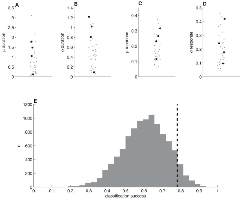
MB population responses to natural and monomolecular odors are indistinguishable. A. Mean response duration (imaging frames) for natural odors (black circles) and monomolecular odors (gray points). B. Standard deviation of response duration. C. Mean evoked response magnitude. D. Standard deviation of evoked response magnitudes. E. LDA-based classification accuracy of natural and monomolecular responses (78%, dashed black bar) compared against chance performance (gray histogram). Observed classification performance was not significantly greater than that of 10,000 chance bootstrap replicates.

We tested whether the magnitude or duration of the odor response could predict whether the stimulus was a natural or monomolecular odorant. To quantify response duration and how consistent this duration is across cells, we calculated the mean and the standard deviation of the number of imaging frames in which the dF/F timecourse of cells were above response threshold (Figure 8A-B). To determine whether natural odors activate the same number of cells but evoke a stronger response at these cells, we calculated the mean evoked response per cell (Figure 8C) and the standard deviation of the mean evoked response (Figure 8D). These parameters did not appear to separate natural and monomolecular odors. Nevertheless, to maximize our chances of finding a difference, we conducted a linear discriminant analysis (LDA) on all four variables simultaneously. LDA is a classification technique which takes into account multiple variables and their interactions in order to best classify two or more groups of data; in this case statistics of responses to monomolecular or natural odorants. We ran the classifier using a leave-one-out cross-validation in order to avoid over-fitting. The resulting classification success was 78% (Figure 8E). We assessed the significance of this low classification accuracy by re-running the classifier 10,000 times with randomized odor labels, so there was no longer any relationship between the response parameters and the identity of the odors. The resulting distribution of classification success is shown in Figure 8E. The observed classification success is well within the range of the randomized values, indicating that natural and monomolecular odors do not evoke fundamentally different responses in KCs.

Discussion

We measured odor-evoked neural activity in the Drosophila MB using two-photon calcium imaging. Monomolecular odorants evoked sparse responses across the KC population. Activity remained sparse in response to multimolecular odor blends, complex natural odors, and even changes in odor concentration. Thus, sparseness was relatively unaltered despite large changes in stimulus complexity and intensity. This robustness is significant because sparse representations are thought to be important for information storage (Marr, 1969; Kanerva, 1988) and the MB plays a critical role in olfactory learning and memory (Erber et al., 1980; Heisenberg et al., 1985). Interestingly, unlike other sensory systems, we found that the MB encodes natural and artificial odors in a similar format. Furthermore, we found that KCs were not spatially organized according to responsiveness or odor tuning and that responsive KCs appeared to be distributed randomly within the cell body layer. We find no evidence of either functional or structural specialization within the MB, rather the main processing feature is to generate sparse stimulus representations.

Spatial organization and tuning curve topography of sparse responses

There is prominent spatial organization to the first two layers of the insect olfactory system. ORNs and PNs project to specific glomeruli that can be uniquely identified across different flies and have predictable response properties. However, it is unclear what role this spatial order plays in sensory processing, and whether it is preserved in the MB. Functional imaging is ideally suited to addressing this question, however the reporter used must be sufficiently sensitive to detect most or all activity in the cells of interest. This appears to be the case in our preparation since the fraction of odor-responsive cells detected with GCaMP3 was similar to that detected using electrophysiological techniques (Turner et al., 2008). This is likely because, although KCs fire a small number of spikes, typically 5 to 10, evoked spike rates are high and spontaneous firing is extremely rare (Turner et al., 2008). Thus, our study provides a far more complete picture of the MB than previous work using the early generation calcium indicator, GCaMP1.3 (Wang et al., 2004), which found that only a tiny fraction of KCs responded to odors. Imaging of PN and KC responses in the honeybee using a synthetic calcium indicator corroborates our imaging results from Drosophila, and highlights the dramatic sparsening that occurs in MB (Szyszka et al., 2005). However, previous studies did not analyze simultaneously recorded neurons to address the topography of odor representations or examine the robustness of sparseness across different stimulus features.

Previous electrophysiological studies showed that most MB neurons did not respond to any odor tested, while some KCs responded to multiple odors (Perez-Orive et al., 2002; Turner et al., 2008). This skewed distribution of response probabilities was also evident in our imaging results. However, electrophysiological recordings are unable to rule out the possibility that responsive neurons form spatially localized clusters. Using a bootstrapping approach, we showed that responsive neurons are in fact arranged randomly within the imaging fields we examined. PNs send axons to distinct but rather large zones within the KC dendritic field in the calyx (Tanaka et al., 2004; Jefferis et al., 2007; Lin et al., 2007). Although the spatial precision is certainly not to the level of individual KCs (Murthy et al., 2008), it is nevertheless conceivable that nearby KCs will have similar tuning curves. Even so, we again found that the relationship between the spatial arrangement of KCs and their response properties was random. Although we cannot rule out the possibility that KC responses are organized along a spatial axis we do not sample with imaging, our results suggest that neither overall responsiveness nor tuning curve shape are spatially organized at the level of the MB.

The vertebrate piriform cortex also displays this absence of functional topography (Stettler and Axel, 2009). In contrast, there is clear anatomical evidence for spatial segregation in other areas at this depth in the olfactory pathway. Mitral cell projections are segregated to distinct zones in amygdala (Sosulski et al.) and anterior olfactory nucleus pars externa (AON) (Ghosh et al.). Similarly, in Drosophila, PN projections within the lateral horn appear more stereotyped than those in the MB (Tanaka et al., 2004; Jefferis et al., 2007; Lin et al., 2007). There is also clear functional segregation between projection patterns of food- and pheromone-responding PNs in the lateral horn (Jefferis et al., 2007). These lines of evidence suggest that the olfactory system may strive to construct odor representations that are heavily experience-based in piriform cortex and MB, while in parallel forming innate representations of odor quality in amygdala, AON and lateral horn.

Robustness of sparse representations to stimulus intensity and complexity

Although sparse coding is useful for learning and memory, an important underlying assumption is that sparseness is robust to naturally varying features of the stimuli, including stimulus intensity and complexity. We tested this by examining sparseness of MB responses to a wide variety of odors, including complex odors composed of multiple components at a range of different concentrations. By examining a broad array of odors, our goal was to uncover whether the MB is in some way tuned to particular stimuli that drive fundamentally different, potentially dense, patterns of activity.

The degree of MB sparseness was weakly correlated with the total population activity in the ORNs. Although there are clearly gain control mechanisms in the antennal lobe that act to normalize different levels of ORN input (Olsen and Wilson, 2008; Root et al., 2008), our results indicate that this process is not complete since net input to the system influences the extent of activity in the MB. Consequently, we examined how robust MB responses were to changes in stimulus intensity. We found that response sparseness was relatively concentration invariant. Within the concentration range that we tested, the proportion of responding KCs remained below 0.2, much lower than the levels observed in the antennal lobe PNs (Wilson et al., 2004). Interestingly, this upper limit is similar to that observed in piriform cortex (Stettler and Axel, 2009).

Using a population imaging approach yielded an unexpected observation: stimulus history had a significant effect on sparseness. It appears that an adaptive process influences sparseness levels, whereby adaptation to strong sensory drive affects subsequent responses to weaker stimuli. When stimuli are presented in a series of increasing concentration steps, sparseness levels in the MB are essentially concentration-invariant. This could be a useful feature for a brain area involved in learning and memory, enabling accurate memory retrieval across a range of concentrations (Masek and Heisenberg, 2008; Yarali et al., 2009). Alternatively, this process may play a role in odor localization; when closing in on an odor source, plume hits of increasing concentration would give a constant level of MB activation, but decreasing concentrations would cause a detectable drop in MB responses. This drop could be a signal to begin casting behavior to search again for the plume (Budick and Dickinson, 2006; Duistermars et al., 2009).

Many sensory systems appear to be optimized for processing natural stimuli. There are examples in the auditory and visual systems where neurons transmit more information about stimuli with natural statistics than artificial stimuli (Rieke et al., 1995; Machens et al., 2001; Yu et al., 2005; Garcia-Lazaro et al., 2006). The olfactory system has clearly evolved to process naturally occurring smells composed of many compounds. We therefore examined how the complexity of an odor affected the sparseness of MB responses. Using monomolecular odors to study a deeper brain area such as the MB may yield an impoverished view of the cellular response properties, just as our understanding of inferotemporal cortex would be limited if the test stimuli were only spots and bars of light, rather than meaningful visual objects. Additionally, anatomical evidence suggests that multimolecular blends could be particularly effective stimuli for KCs. PN projections are widely overlapping in the calyx, suggesting that individual KCs receive convergent input from multiple different PN types. Thus, KCs could be tuned to detect coincident input from particular combinations of active PNs.

We examined MB responses to a variety of different natural odors, including smells of ripe fruits. At the ORN layer, it is possible to distinguish fruit odors from monomolecular odors when viewed at the population level (Hallem and Carlson, 2006). We tested whether this distinction was detectable in the MB population. Interestingly, we found that no aspect of the response to natural smells enabled us to differentiate them from monomolecular odors. Moreover, the sparseness of natural odor representations was indistinguishable from that of monomolecular smells. This likely arises because the responses to individual components in a multi-component blend are strongly sub-additive. Overall, these results indicate that MB representations are not specialized for naturally occurring odors, even though these stimuli drive strong behavioral responses (Stensmyr et al., 2003; Fishilevich et al., 2005; Budick and Dickinson, 2006). The indistinguishability of natural and artificial odors reinforces the view that the MB is a purely associative brain center.

Both the functional and anatomical similarities between the antennal lobe and olfactory bulb in mammals are well established and striking. A recent report suggests that the invertebrate MB is phylogenetically homologous to neocortex, based on expression patterns of important developmental genes (Tomer et al., 2010). Using detailed functional imaging, we have shown a striking functional similarity between the mushroom body and earlier reports of piriform cortex (Stettler and Axel, 2009). These results suggest that the fundamental feature of olfactory processing at this layer of the system is to create sparse representations in a way that is robust to variation in the features of the olfactory stimulus.

References

- Aso Y, Grubel K, Busch S, Friedrich AB, Siwanowicz I, Tanimoto H. The mushroom body of adult Drosophila characterized by GAL4 drivers. J Neurogenet. 2009;23:156–172. doi: 10.1080/01677060802471718. [DOI] [PubMed] [Google Scholar]
- Bhandawat V, Olsen SR, Gouwens NW, Schlief ML, Wilson RI. Sensory processing in the Drosophila antennal lobe increases reliability and separability of ensemble odor representations. Nat Neurosci. 2007;10:1474–1482. doi: 10.1038/nn1976. [DOI] [PMC free article] [PubMed] [Google Scholar]
- Broome BM, Jayaraman V, Laurent G. Encoding and decoding of overlapping odor sequences. Neuron. 2006;51:467–482. doi: 10.1016/j.neuron.2006.07.018. [DOI] [PubMed] [Google Scholar]
- Budick SA, Dickinson MH. Free-flight responses of Drosophila melanogaster to attractive odors. J Exp Biol. 2006;209:3001–3017. doi: 10.1242/jeb.02305. [DOI] [PubMed] [Google Scholar]
- Connolly JB, Roberts IJ, Armstrong JD, Kaiser K, Forte M, Tully T, O’Kane CJ. Associative learning disrupted by impaired Gs signaling in Drosophila mushroom bodies. Science. 1996;274:2104–2107. doi: 10.1126/science.274.5295.2104. [DOI] [PubMed] [Google Scholar]
- Duistermars BJ, Chow DM, Frye MA. Flies require bilateral sensory input to track odor gradients in flight. Curr Biol. 2009;19:1301–1307. doi: 10.1016/j.cub.2009.06.022. [DOI] [PMC free article] [PubMed] [Google Scholar]
- Erber J, Masuhr T, Menzel R. Localization of Short-Term-Memory in the Brain of the Bee, Apis-Mellifera. Physiological Entomology. 1980;5:343–358. [Google Scholar]
- Fishilevich E, Domingos AI, Asahina K, Naef F, Vosshall LB, Louis M. Chemotaxis behavior mediated by single larval olfactory neurons in Drosophila. Curr Biol. 2005;15:2086–2096. doi: 10.1016/j.cub.2005.11.016. [DOI] [PubMed] [Google Scholar]
- Garcia-Lazaro JA, Ahmed B, Schnupp JW. Tuning to natural stimulus dynamics in primary auditory cortex. Curr Biol. 2006;16:264–271. doi: 10.1016/j.cub.2005.12.013. [DOI] [PubMed] [Google Scholar]
- Ghosh S, Larson SD, Hefzi H, Marnoy Z, Cutforth T, Dokka K, Baldwin KK. Sensory maps in the olfactory cortex defined by long-range viral tracing of single neurons. Nature. 472:217–220. doi: 10.1038/nature09945. [DOI] [PubMed] [Google Scholar]
- Guizar-Sicairos M, Thurman ST, Fienup JR. Efficient subpixel image registration algorithms. Opt Lett. 2008;33:156–158. doi: 10.1364/ol.33.000156. [DOI] [PubMed] [Google Scholar]
- Hallem EA, Carlson JR. Coding of odors by a receptor repertoire. Cell. 2006;125:143–160. doi: 10.1016/j.cell.2006.01.050. [DOI] [PubMed] [Google Scholar]
- Heisenberg M, Borst A, Wagner S, Byers D. Drosophila mushroom body mutants are deficient in olfactory learning. J Neurogenet. 1985;2:1–30. doi: 10.3109/01677068509100140. [DOI] [PubMed] [Google Scholar]
- Jayaraman V, Laurent G. Evaluating a genetically encoded optical sensor of neural activity using electrophysiology in intact adult fruit flies. Front Neural Circuits. 2007;1:3. doi: 10.3389/neuro.04.003.2007. [DOI] [PMC free article] [PubMed] [Google Scholar]
- Jefferis GS, Potter CJ, Chan AM, Marin EC, Rohlfing T, Maurer CR, Jr, Luo L. Comprehensive maps of Drosophila higher olfactory centers: spatially segregated fruit and pheromone representation. Cell. 2007;128:1187–1203. doi: 10.1016/j.cell.2007.01.040. [DOI] [PMC free article] [PubMed] [Google Scholar]
- Kanerva P. Sparse Distributed Memory. Cambridge, MA: MIT Press; 1988. [Google Scholar]
- Larsson MC, Domingos AI, Jones WD, Chiappe ME, Amrein H, Vosshall LB. Or83b encodes a broadly expressed odorant receptor essential for Drosophila olfaction. Neuron. 2004;43:703–714. doi: 10.1016/j.neuron.2004.08.019. [DOI] [PubMed] [Google Scholar]
- Lee T, Lee A, Luo L. Development of the Drosophila mushroom bodies: sequential generation of three distinct types of neurons from a neuroblast. Development. 1999;126:4065–4076. doi: 10.1242/dev.126.18.4065. [DOI] [PubMed] [Google Scholar]
- Lin HH, Lai JS, Chin AL, Chen YC, Chiang AS. A map of olfactory representation in the Drosophila mushroom body. Cell. 2007;128:1205–1217. doi: 10.1016/j.cell.2007.03.006. [DOI] [PubMed] [Google Scholar]
- Machens CK, Stemmler MB, Prinz P, Krahe R, Ronacher B, Herz AV. Representation of acoustic communication signals by insect auditory receptor neurons. J Neurosci. 2001;21:3215–3227. doi: 10.1523/JNEUROSCI.21-09-03215.2001. [DOI] [PMC free article] [PubMed] [Google Scholar]
- Marr D. A theory of cerebellar cortex. J Physiol. 1969;202:437–470. doi: 10.1113/jphysiol.1969.sp008820. [DOI] [PMC free article] [PubMed] [Google Scholar]
- Martinez WL, Martinez AL. Exploratory Data Analysis with Matlab. London: Chapman and Hall; 2005. [Google Scholar]
- Masek P, Heisenberg M. Distinct memories of odor intensity and quality in Drosophila. Proc Natl Acad Sci U S A. 2008;105:15985–15990. doi: 10.1073/pnas.0804086105. [DOI] [PMC free article] [PubMed] [Google Scholar]
- Meredith M. Patterned response to odor in mammalian olfactory bulb: the influence of intensity. J Neurophysiol. 1986;56 doi: 10.1152/jn.1986.56.3.572. [DOI] [PubMed] [Google Scholar]
- Moskowitz HR, Barbe CD. Profiling of odor components and their mixtures. Sens Processes. 1977;1:212–226. [PubMed] [Google Scholar]
- Murthy M, Turner GC. In vivo whole-cell recordings in the Drosophila brain. In: Zhang BZ, Waddell S, Freeman M, editors. Drosophila neurobiology methods: a laboratory manual. Cold Spring Harbor, NY: Cold Spring Harbor Laboratory Press; 2010. [Google Scholar]
- Murthy M, Fiete I, Laurent G. Testing odor response stereotypy in the Drosophila mushroom body. Neuron. 2008;59:1009–1023. doi: 10.1016/j.neuron.2008.07.040. [DOI] [PMC free article] [PubMed] [Google Scholar]
- Olsen SR, Wilson RI. Lateral presynaptic inhibition mediates gain control in an olfactory circuit. Nature. 2008;452:956–960. doi: 10.1038/nature06864. [DOI] [PMC free article] [PubMed] [Google Scholar]
- Olsen SR, Bhandawat V, Wilson RI. Divisive normalization in olfactory population codes. Neuron. 2010;66:287–299. doi: 10.1016/j.neuron.2010.04.009. [DOI] [PMC free article] [PubMed] [Google Scholar]
- Olshausen BA, Field DJ. Sparse coding of sensory inputs. Curr Opin Neurobiol. 2004;14:481–487. doi: 10.1016/j.conb.2004.07.007. [DOI] [PubMed] [Google Scholar]
- Perez-Orive J, Mazor O, Turner GC, Cassenaer S, Wilson RI, Laurent G. Oscillations and sparsening of odor representations in the mushroom body. Science. 2002;297:359–365. doi: 10.1126/science.1070502. [DOI] [PubMed] [Google Scholar]
- Pinheiro JC, Bates DM. Mixed-effects models in S and S-plus. Springer; 2000. [Google Scholar]
- Rieke F, Bodnar DA, Bialek W. Naturalistic stimuli increase the rate and efficiency of information transmission by primary auditory afferents. Proc Biol Sci. 1995;262:259–265. doi: 10.1098/rspb.1995.0204. [DOI] [PubMed] [Google Scholar]
- Root CM, Masuyama K, Green DS, Enell LE, Nassel DR, Lee CH, Wang JW. A presynaptic gain control mechanism fine-tunes olfactory behavior. Neuron. 2008;59:311–321. doi: 10.1016/j.neuron.2008.07.003. [DOI] [PMC free article] [PubMed] [Google Scholar]
- Silbering AF, Galizia CG. Processing of odor mixtures in the Drosophila antennal lobe reveals both global inhibition and glomerulus-specific interactions. J Neurosci. 2007;27:11966–11977. doi: 10.1523/JNEUROSCI.3099-07.2007. [DOI] [PMC free article] [PubMed] [Google Scholar]
- Sosulski DL, Lissitsyna Bloom M, Cutforth T, Axel R, Datta SR. Distinct representations of olfactory information in different cortical centres. Nature. 472:213–216. doi: 10.1038/nature09868. [DOI] [PMC free article] [PubMed] [Google Scholar]
- Stensmyr MC, Giordano E, Balloi A, Angioy AM, Hansson BS. Novel natural ligands for Drosophila olfactory receptor neurones. J Exp Biol. 2003;206:715–724. doi: 10.1242/jeb.00143. [DOI] [PubMed] [Google Scholar]
- Stettler DD, Axel R. Representations of odor in the piriform cortex. Neuron. 2009;63:854–864. doi: 10.1016/j.neuron.2009.09.005. [DOI] [PubMed] [Google Scholar]
- Stopfer M, Laurent G. Short-term memory in olfactory network dynamics. Nature. 1999;402:664–668. doi: 10.1038/45244. [DOI] [PubMed] [Google Scholar]
- Stopfer M, Jayaraman V, Laurent G. Intensity versus identity coding in an olfactory system. Neuron. 2003;39:991–1004. doi: 10.1016/j.neuron.2003.08.011. [DOI] [PubMed] [Google Scholar]
- Szyszka P, Galkin A, Menzel R. Associative and non-associative plasticity in kenyon cells of the honeybee mushroom body. Front Syst Neurosci. 2008;2:3. doi: 10.3389/neuro.06.003.2008. [DOI] [PMC free article] [PubMed] [Google Scholar]
- Szyszka P, Ditzen M, Galkin A, Galizia CG, Menzel R. Sparsening and temporal sharpening of olfactory representations in the honeybee mushroom bodies. J Neurophysiol. 2005;94:3303–3313. doi: 10.1152/jn.00397.2005. [DOI] [PubMed] [Google Scholar]
- Tabor R, Yaksi E, Weislogel JM, Friedrich RW. Processing of odor mixtures in the zebrafish olfactory bulb. J Neurosci. 2004;24:6611–6620. doi: 10.1523/JNEUROSCI.1834-04.2004. [DOI] [PMC free article] [PubMed] [Google Scholar]
- Tanaka NK, Awasaki T, Shimada T, Ito K. Integration of chemosensory pathways in the Drosophila second-order olfactory centers. Curr Biol. 2004;14:449–457. doi: 10.1016/j.cub.2004.03.006. [DOI] [PubMed] [Google Scholar]
- Tian L, Hires SA, Mao T, Huber D, Chiappe ME, Chalasani SH, Petreanu L, Akerboom J, McKinney SA, Schreiter ER, Bargmann CI, Jayaraman V, Svoboda K, Looger LL. Imaging neural activity in worms, flies and mice with improved GCaMP calcium indicators. Nat Methods. 2009;6:875–881. doi: 10.1038/nmeth.1398. [DOI] [PMC free article] [PubMed] [Google Scholar]
- Tomer R, Denes AS, Tessmar-Raible K, Arendt D. Profiling by image registration reveals common origin of annelid mushroom bodies and vertebrate pallium. Cell. 2010;142:800–809. doi: 10.1016/j.cell.2010.07.043. [DOI] [PubMed] [Google Scholar]
- Turner GC, Bazhenov M, Laurent G. Olfactory representations by Drosophila mushroom body neurons. J Neurophysiol. 2008;99:734–746. doi: 10.1152/jn.01283.2007. [DOI] [PubMed] [Google Scholar]
- Wang Y, Guo HF, Pologruto TA, Hannan F, Hakker I, Svoboda K, Zhong Y. Stereotyped odor-evoked activity in the mushroom body of Drosophila revealed by green fluorescent protein-based Ca2+ imaging. J Neurosci. 2004;24:6507–6514. doi: 10.1523/JNEUROSCI.3727-03.2004. [DOI] [PMC free article] [PubMed] [Google Scholar]
- Willmore B, T D. Characterizing the sparseness of neural codes. Network: Comput Neural Syst. 2001;12:255–270. [PubMed] [Google Scholar]
- Wilson RI, Turner GC, Laurent G. Transformation of olfactory representations in the Drosophila antennal lobe. Science. 2004;303:366–370. doi: 10.1126/science.1090782. [DOI] [PubMed] [Google Scholar]
- Yarali A, Ehser S, Hapil FZ, Huang J, Gerber B. Odour intensity learning in fruit flies. Proc Biol Sci. 2009;276:3413–3420. doi: 10.1098/rspb.2009.0705. [DOI] [PMC free article] [PubMed] [Google Scholar]
- Yu Y, Romero R, Lee TS. Preference of sensory neural coding for 1/f signals. Phys Rev Lett. 2005;94:108103. doi: 10.1103/PhysRevLett.94.108103. [DOI] [PubMed] [Google Scholar]