

Abstract
A study of Biphasic contact of soft tissues is fundamental to understanding the biomechanical behavior of human diarthrodial joints. To date, biphasic-biphasic contact has been developed for idealized geometries and not been accessible for more general geometries. In this paper, a finite element formulation is developed for contact of biphasic tissues. The Augmented Lagrangian method is used to enforce the continuity of contact traction and fluid pressure across the contact interface, and the resulting method is implemented in the commercial software COMSOL Multiphysics. The accuracy of the implementation is verified using 2D axisymmetric problems, including indentation with a flat-ended indenter, indentation with spherical-ended indenter, and contact of glenohumeral cartilage layers. The biphasic finite element contact formulation and its implementation are shown to be robust and able to handle physiologically relevant problems.
Keywords: Biphasic Contact, Soft tissue, Cartilage, Augmented Lagrangian Method
1 Introduction
Understanding the biomechanical behavior of human diarthrodial joints is essential to better diagnostic techniques, improved surgical interventions, and engineering of tissue replacements. The study of contact of soft tissue layers is fundamental to this understanding. Analytical solutions for the biphasic contact mechanics in axisymmetric joints have been developed [1–4], but these solutions apply, understandably, to fairly idealized problems. In order to analyze the contact mechanics in physiological joints, where geometry is far more complex, it is necessary to use numerical approximation methods, such as the finite element method. However, only a limited number of studies have addressed these types of problems, and numerical computation of the soft tissue contact mechanics remains challenging.
Three classes of methods have been used to enforce the contact conditions in single-phase contact problems: the penalty method, Lagrange multiplier method, and augmented Lagrangian method. The augmented Lagrangian method incorporates strong features from the penalty and Lagrange multiplier methods, and is more robust than either individual method [5]. Beside the equality conditions for displacement and traction that a single-phase contact problem consists of, there are two additional equality conditions on relative fluid flow and pressure in the biphasic contact problem [6]. Therefore, it is not viable to directly adopt one of the three methods for the biphasic contact problem. Spilker and coworkers [7–9] developed a Lagrange multiplier method to investigate the contact mechanics of biphasic cartilage layers in 2D and 3D under small deformations. Chen et al. and Ateshian et al. investigated contact mechanics of biphasic cartilage layers under large deformations and sliding using a Lagrange multiplier method [10] and an augmented Lagrangian method [11], respectively.
ABAQUS is a program widely used to study soft tissue contact [12–16]. Though the program provides many powerful features, its biphasic contact implementation exhibits significant limitations. First, the ‘drainage-only-flow’ boundary condition (i.e. the fluid only flows from the interior to the exterior of the cartilage layer) is inconsistent with the equation of conservation of mass across the contact interface [6]. Second, the software is unable to automatically enforce the free-draining condition outside of the contact area. This limitation needs to be addressed by a user-defined routine [13].
To date, there have been no successful developments of biphasic finite element contact analysis for 3D geometries of physiological joints. Our long-term goal is to create experimentally validated, 3D computational models of the knee and other joint, including proper modeling of the biphasic contact problem. The objective of this paper is to develop a finite element contact formulation for soft tissue, using an augmented Lagrangian method to enforce the continuity of contact traction and fluid pressure across the contact interface. The finite element contact formulation is implemented in COMSOL Multiphysics, which can be later extended for the necessary 3D geometries. Several example problems are provided to verify the accuracy of the implementation.
2 Methods
Consider two deformable bodies, labeled A and B, with boundaries ΓA and ΓB, under the assumption of infinitesimal deformation. The two bodies are in frictionless contact over portions of ΓA and ΓB denoted by γA and γB, respectively. A standard continuum mechanics nomenclature is adopted, and the indicial notation is used.
2.1 Biphasic Continuum Equations for Soft Tissues
The mixed velocity-pressure (v-p) formulation of linear biphasic theory [17] is adopted in this study. The governing equations most amenable to this formulation are
| (1) |
| (2) |
where superscripts s and f refer to the solid and fluid phases, respectively; is the solid phase velocity, which is the time derivative of the solid phase displacements ; k is the permeability; p is the fluid pressure; (),i denotes the partial derivative; and are the solid and fluid phase stress tensors; is the solid phase strain tensor (the superscript s is omitted); is the material property tensor of the solid phase; and δij is the Kronecker delta. In addition, there are constitutive relations for each phase
| (3) |
| (4) |
where φs and φf are the solid and fluid volume fractions, respectively, for the saturated (φs + φf = 1) mixture.
The initial and boundary conditions on the non-contacting boundaries of bodies A and B (we drop the superscripts A and B for these equations) are
| (5) |
| (6) |
| (7) |
| (8) |
| (9) |
where an over-bar signifies a prescribed value of the quality; the subscript ()0 denotes an initial value; total stress is defined as the sum of the fluid and solid stress, ; and the relative fluid flow is defined as or Q = −κ p,i n,i. The boundaries Γβ, β=u, v, p, t, and Q, correspond to portions on which displacement, velocity, pressure, total traction, and relative flow, respectively, are prescribed. Note that these boundary portions apply to either body A or body B, and that they do not apply to the contact boundaries γA and γB.
2.2 Biphasic Contact Modeling
Contact boundary conditions are taken from the theoretical work of Hou et al. (1989). Contact boundary conditions defined on the boundaries γA and γB are
| (10) |
| (11) |
| (12) |
| (13) |
These equations correspond to kinematic conditions on the continuity of location of points in contact, Eq. (10); continuity of the relative flow across the contact boundary, Eq. (11); kinetic continuity conditions on the fluid pressure, Eq. (12); and the normal component of solid phase elastic stress, Eq. (13), on the contact boundary.
To enforce the contact constraint based on augmented Lagrangian method, let the normal component of the contact pressure be given by
| (14) |
where g is the gap distance from the destination boundary γB to the source boundary γA in the direction normal to the destination surface, and ηn is the normal penalty factor with units of force per volume. As the boundaries approach one another, the source point XA converges to the closest destination point XB. The augmented Lagrangian method ensures that the contact boundaries overlap by an acceptably negligible amount g as the penalty factor goes to infinity.
The augmented Lagrangian framework for single-phase contact problem [5] was adapted to the current biphasic contact framework (Table 1). An augmentation component is introduced for the contact pressure tn, and an additional iteration level is added where the usual displacement and fluid pressure variables are solved separately from the contact pressure. The algorithm repeats this procedure until it fulfills a convergence criterion.
Table 1.
Augmented Lagrangian algorithm for biphasic contact of soft tissues
|
GTOL is the tolerance for gap distance
The biphasic contact equations were implemented in commercial finite element software (COMSOL Multiphysics 4.1®, COMSOL, Inc., Burlington, MA). As with earlier biphasic implementations in COMSOL [18], solid mechanics in the Structural Mechanics Module and Darcy’s Law in the Earth Science Module were used and coupled to obtain the linear biphasic equations. The Contact Pair feature was used to enforce contact constraint for the solid phase and the Identity Pair feature was used to enforce fluid continuity constraint for the fluid phase. The penalty factor was set as E/hm*c, where E is the elastic modulus of the materials, hm is the mesh size, and c is a user-defined constant with typical range of 0.1 to 10.
3 Example Problems
3.1 Indentation Test with Flat-Ended Indenter
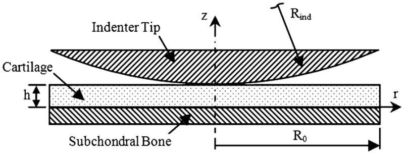
Figure 1 illustrates the indentation with a flat-ended indenter which is modeled as 2D axisymmetric problem. A layer of soft tissue of uniform thickness, h=0.75 mm, is attached to subchondral bone at its lower surface, and indented normal to the tissue surface by a flat-ended cylindrical indenter of radius and height, Rind =0.75mm. The radius of soft tissue is R0=4Rind mm since a previous study has demonstrated that the tissue response is negligible for R0>4Rind [19]. The subchondral bone is modeled as an impermeable, fixed boundary. The top of the indenter is subjected to a displacement of −0.075mm applied in a ramp time of 500s and then held. A free-draining boundary condition is applied on the top of the indenter and on the cartilage surface outside of the contact area. Material properties of the cartilage are Young’s modulus EA = 0.5417MPa, Poisson’s ratio νA = 0.0833, permeability κA = 4.0 × 10⁻¹⁵ m4/N/s, and solid content φsA = 0.2. Material properties of the indenter are EB = 541.7MPa, νB = 0.125, κB =4.0 × 10⁻¹²m4/N/s, and φsB = 0.95. The model was discretized with a total of 2387 triangular element. The bottom boundary of the indenter was set as source boundary, and the top boundary of the cartilage was set as destination boundary.
Fig. 1.

A schematic diagram of the biphasic indentation test with a flat-ended cylindrical indenter.
Results on axial stress σz, axial strain εz, shear stress σrz, and fluid pressure p, at several depths are compared to Spilker et al. (1992), and they are in good agreement (Fig. 2). For axial stress and strain at top level of the tissue, smooth distribution is found under the loaded surface; minimum values are found at the edge of the indenter; the stress and strain increase rapidly to zero where r>Rind. Shear stress at top level of the tissue has a similar distribution except that it increases rapidly to a maximum value at the indenter edge and then decreases rapidly to zero for r>Rind. Axial stress, axial strain and shear stress at the mid-thickness and bottom surface of the tissue vary smoothly with no boundary layers. In contrast to the stress and strain components, the fluid pressure increases with increasing depth, and varies smoothly.
Fig. 2.

The (A) axial stress σz, (B) axial strain εz, (C) shear stress σrz, and (D) fluid pressure, p at several depths predicted by the biphasic contact finite element model and the model of Spilker et al. (1992).
Distributions of fluid pressure, p, (Fig. 3A) and axial stress, σz, (Fig. 3C) are in good agreement with results of 3D contact finite element solution of this axisymmetric problem published by Yang and Spilker (2007). Large fluid pressure is found at the mid-thickness and bottom surface of the tissue under loaded area, and fluid pressure is negligible at the indenter and the tissue where r>2Rind. Very large negative axial stress is found at the edge of the indenter. Negligible axial stress is found in the tissue for r>Rind. For the primary parameters, displacement (result not shown, since the uniform displacement is essentially prescribed through the rigid indenter) and fluid pressure (Fig. 3B), the continuity conditions are accurately satisfied. For the derived quantity, axial stress (Fig. 3D), good agreement is also observed.
Fig. 3.

(A and C) distribution of fluid pressure p and axial stress σz (in kPa) at 250s on the deformed geometry, red arrows indicate fluid velocity. (B and D) continuity of fluid pressure and axial stress between the two bodies along the contact boundary at 250s.
3.2 Indentation Test with Spherical-ended Indenter
Figure 4 illustrates the indentation test with a spherical-ended cylindrical indenter and it is modeled as 2D axisymmetric problem. The indenter radius is Rind=100mm, radius of the cartilage is R0=20mm, and thickness of the cartilage is h=1mm. The subchondral bone is modeled as an impermeable, fixed boundary. The top of indenter is subjected to a displacement of −0.04mm applied in a ramp time of 100s and then held, and a no-flow boundary condition is set for the top of the indenter. A free draining boundary condition is applied on the cartilage surface outside of the contact area. The material properties of the cartilage are Young’s modulus EA = 0.5MPa, Poisson’s ratio νA = 0, permeability κA = 2.0 × −15m4/N/s, and solid content φsA = 0.25. Material properties of the rigid impermeable indenter are EB = 500MPa, νB = 0.125, κB = 2.0 × −18m4/N/s, and φsB = 0.99. The model was discretized with a total of 2978 triangular elements. The curved boundary of the indenter tip was set as source boundary, and the top boundary of the cartilage was set as destination boundary.
Fig. 4.
A schematic diagram of the biphasic indentation test with a spherical-ended cylindrical indenter.
Results of axial displacement and fluid pressure (Fig. 5) show good agreement with that of 2D axisymmetric and 3D model of this axisymmetric problem based on Lagrange multiplier method [7, 9]. Tensile displacement is found on cartilage surface beside the contact area. This region also experiences an efflux of fluid as depicted by the fluid velocity (Fig. 5B). Fluid pressure is fairly uniform through the depth. Maximum fluid pressure is found at the center and decreases toward the edge of contact. The continuity condition for fluid pressure is satisfied along the contact surface.
Fig. 5.

Distribution of axial displacement (A, in mm) and fluid pressure (B, in kPa) at 100s on deformed geometry, red arrows indicate fluid velocity (B).
The normal traction along the contact surface at t=100s is compared to results published by Donzelli and Spilker (1998), and they are in good agreement (Fig. 6). Fluid traction is nearly twice the solid traction, indicating that the fluid phase carries twice the load of the solid phase on the contact surface. As the fluid flow diminishes with time, the fluid pressure will decrease, and the total load is increasingly carried by the solid phase.
Fig. 6.

Normal traction distributions along the top boundary of cartilage at 100s in the biphasic indentation test with a spherical-ended indenter. Lines are the results of finite element contact solution using augmented Lagrangian method, and symbols are results of finite element solution based on Lagrange multiplier method [7].
3.3 Glenohumeral Joint Contact
A physiologically relevant problem, the glenohumeral joint contact of the human shoulder (Fig. 7), is modeled as a 2D axisymmetric problem. The idealized glenoid and humeral head cartilage layers are modeled based on the average values of stereophotogrammetric data [20]. The thickness of the two cartilage layers at center are h1=h2=1.5mm, and the width of the glenoid and the humeral head are w1=11.5mm and w2=19.1mm, respectively. Radiuses of the glenoid cartilage are R1=34.5mm and R2=26mm. The humeral head cartilage is uniformly thick and its radius is R3=23.5mm. Impermeable boundary conditions are applied to the cartilage-bone interface instead of explicit modeling of the subchondral bones. The humerus-bone interface is subjected to a compressive axial displacement of 0.2mm applied in a ramp time of 10s and then held. The glenoid-bone interface is held fixed. A free draining boundary condition is applied on the right boundary of the cartilage layers and on the cartilage surface outside of the contact area. The material properties of the glenoid cartilage are Young’s modulus EA = 0.559MPa, Poisson’s ratio νA = 0.02, permeability κA =1.16−15m4/N/s, and solid content φsA = 0.2. The material properties of the humeral head cartilage are Young’s modulus EB = 0.5565MPa, Poisson’s ratio νB = 0.05, permeability κB =1.7 × −15m4/N/s, and solid content φsB = 0.2. The model was discretized with total of 3494 triangular elements. The bottom boundary of the humeral head cartilage layer was set as source boundary, and the top boundary of the glenoid cartilage layer was set as destination boundary.
Fig. 7.

A schematic diagram of axisymmetric glenohumeral joint in contact. Regions with dots represent cartilage layers, and open regions are bone.
Axial displacement on deformed geometry (Fig. 8) shows good agreement with the results of 3D finite element solution based on the Lagrange multiplier method [9]. The contact surface evolves with time as the compressive axial displacement increases. The tissue surface undergoes a tensile deformation in the outer portion of the contact surface.
Fig. 8.

Axial displacement (in mm) of the shoulder cartilage on deformed geometry at 5s (A) and 10s (B). Boundary lines are initial position.
Fluid pressure distribution (Fig. 9A) agrees with the results of 3D finite element solution published by Yang and Spilker (2007). Maximum fluid pressure is found at the center of the cartilage layers and decreases toward the edge of contact. Continuity condition for fluid pressure across contact interface is accurately satisfied. As 0.2mm compressive axial displacement applied on the glenohumeral joint, approximately 87% of the glenoid surface is in contact with the humeral head, and a majority of the load is supported by the fluid phase in the contact surface (Fig. 9B).
Fig. 9.

(A) Fluid pressure (in kPa) distribution of the shoulder cartilage on deformed geometry at 10s. (B) Normal traction distribution along top boundary of glenoid cartilage at 10s.
Peak maximum and minimum principal elastic stress occur at the cartilage-bone interface, away from the center (Fig. 10). These peak values have the shape of a circular band and are smaller than the contact radius. The glenoid cartilage has a wider area of peak stresses than the humerus cartilage. These findings agree with the results of the 2D axisymmetric and 3D finite element solution based on the Lagrange multiplier method [8, 9, 21].
Fig. 10.

Distributions of maximum (A) and minimum (B) principal elastic stress (in kPa) on deformed geometry at 10s.
4 Concluding remarks
A biphasic finite element formulation has been developed for the frictionless contact of soft tissues. The mixed v-p formulation of linear biphasic theory was adopted to model soft tissue as a mixture of solid and fluid phases. An augmented Lagrangian method was used to enforce the continuity of contact traction and fluid pressure across the contact interface. The biphasic finite element contact formulation was implemented in COMSOL Multiphysics. The implementation has been verified via several example problems, including indentation with a flat-ended indenter, indentation with a spherical-ended indenter, and contact of idealized glenohumeral cartilage layers. The biphasic finite element contact formulation and its implementation have proven to be robust, and able to handle physiologically relevant problems.
Before the biphasic finite element contact formulation developed in this paper can be used in the analysis of realistic physiological problems of joint contact, it needs to be verified in 3D contact problems. Linear biphasic theory adopted in this study is under the assumption of small deformation, so for studies of soft tissue with large deformation and sliding, geometric nonlinearity should be added in the formulation.
Acknowledgments
This study was supported by a grant from the National Institute of Health (NIH 1R01 AR057343-01A2).
References
- 1.Ateshian GA, Lai WM, Zhu WB, Mow VC. An asymptotic solution for the contact of two biphasic cartilage layers. Journal of Biomechanics. 1994;27:1347–1360. doi: 10.1016/0021-9290(94)90044-2. [DOI] [PubMed] [Google Scholar]
- 2.Ateshian GA, Wang H. A theoretical solution for the frictionless rolling contact of cylindrical biphasic articular cartilage layers. Journal of Biomechanics. 1995;28:1341–1355. doi: 10.1016/0021-9290(95)00008-6. [DOI] [PubMed] [Google Scholar]
- 3.Wu JZ, Herzog W, Epstein M. An improved solution for the contact of two biphasic cartilage layers. Journal of Biomechanics. 1997;30:371–375. doi: 10.1016/s0021-9290(96)00148-0. [DOI] [PubMed] [Google Scholar]
- 4.Wu JZ, Herzog W, Epstein M. Articular joint mechanics with biphasic cartilage layers under dynamic loading. Journal of Biomechanical Engineering. 1998;120:77–84. doi: 10.1115/1.2834310. [DOI] [PubMed] [Google Scholar]
- 5.Simo JC, Laursen TA. An augmented Lagrangian treatment of contact problems involving friction. Computers and Structures. 1992;42:97–116. [Google Scholar]
- 6.Hou JS, Holmes MH, Lai WM, Mow VC. Boundary conditions at the cartilage-synovial fluid interface for joint lubrication and theoretical verifications. Journal of Biomechanical Engineering. 1989;111:78–87. doi: 10.1115/1.3168343. [DOI] [PubMed] [Google Scholar]
- 7.Donzelli PS, Spilker RL. A contact finite element formulation for biological soft hydrated tissues. Computer Methods in Applied Mechanics and Engineering. 1998;153:63–79. [Google Scholar]
- 8.Donzelli PS, Spilker RL, Ateshian GA, Mow VC. Contact analysis of biphasic transversely isotropic cartilage layers and correlations with tissue failure. Journal of Biomechanics. 1999;32:1037–1047. doi: 10.1016/s0021-9290(99)00106-2. [DOI] [PubMed] [Google Scholar]
- 9.Yang T, Spilker RL. A lagrange multiplier mixed finite element formulation for three-dimensional contact of biphasic tissues. Journal of Biomechanical Engineering. 2007;129:457–471. doi: 10.1115/1.2737056. [DOI] [PubMed] [Google Scholar]
- 10.Chen X, Chen Y, Hisada T. Development of a finite element procedure of contact analysis for articular cartilage with large deformation based on the biphasic theory. JSME International Journal Series C: Mechanical Systems, Machine Elements and Manufacturing. 2005;48:537–546. [Google Scholar]
- 11.Ateshian GA, Maas S, Weiss JA. Finite element algorithm for frictionless contact of porous permeable media under finite deformation and sliding. Journal of Biomechanical Engineering. 2010;132:061006. doi: 10.1115/1.4001034. [DOI] [PMC free article] [PubMed] [Google Scholar]
- 12.Federico S, Rosa GL, Herzog W, Wu JZ. Effect of fluid boundary conditions on joint contact mechanics and applications to the modeling of osteoarthritic joints. Journal of Biomechanical Engineering. 2004;126:220–225. doi: 10.1115/1.1691445. (Erratum in: 2005, Journal of Biomedical Engineering 2127, 2205–2209) [DOI] [PubMed] [Google Scholar]
- 13.Pawaskar SS, Fisher J, Jin Z. Robust and general method for determining surface fluid flow boundary conditions in articular cartilage contact mechanics modeling. Journal of Biomechanical Engineering. 2010;132:031001. doi: 10.1115/1.4000869. [DOI] [PubMed] [Google Scholar]
- 14.Pawaskar SS, Ingham E, Fisher J, Jin Z. Fluid load support and contact mechanics of hemiarthroplasty in the natural hip joint. Medical Engineering and Physics. 2011;33:96–105. doi: 10.1016/j.medengphy.2010.09.009. [DOI] [PubMed] [Google Scholar]
- 15.Warner MD, Taylor WR, Clift SE. Finite element biphasic indentation of cartilage: a comparison of experimental indenter and physiological contact geometries. Proceedings of the Institution of Mechanical Engineers. 2001;215:487–496. doi: 10.1243/0954411011536082. [DOI] [PubMed] [Google Scholar]
- 16.Wu JZ, Herzog W, Epstein M. Evaluation of the finite element software ABAQUS for biomechanical modelling of biphasic tissues. Journal of Biomechanics. 1998;31:165–169. doi: 10.1016/s0021-9290(97)00117-6. [DOI] [PubMed] [Google Scholar]
- 17.Almeida ES, Spilker RL. Mixed and penalty finite element models for the nonlinear behavior of biphasic soft tissues in finite deformation: Part I--Alternate formulations. Computer Methods in Biomechanics and Biomedical Engineering. 1997;1:25–46. doi: 10.1080/01495739708936693. [DOI] [PubMed] [Google Scholar]
- 18.Spilker RL, Nickel JC, Iwasaki LR. A biphasic finite element model of in vitro plowing tests of the temporomandibular joint disc. Annals of Biomedical Engineering. 2009;37:1152–1164. doi: 10.1007/s10439-009-9685-2. [DOI] [PubMed] [Google Scholar]
- 19.Spilker RL, Suh JK, Mow VC. A finite element analysis of the indentation stress-relaxation response of linear biphasic articular cartilage. Journal of Biomechanical Engineering. 1992;114:191–201. doi: 10.1115/1.2891371. [DOI] [PubMed] [Google Scholar]
- 20.Soslowsky IJ, Ateshian GA, Mow VC. Stereophotogrammetric determination of joint anatomy and contact areas. In: Mow VC, Ratcliffe TA, Woo SL, editors. Biomechanics of Diarthrodial Joints. Springer-Verlag; Berlin: 1990. pp. 243–268. [Google Scholar]
- 21.Donzelli PS. PhD thesis. Rensselaer Polytechnic Institute; Troy, NY: 1995. A mixed-penalty contact finite element formulation for biphasic soft tissue. [Google Scholar]