Deterministic and Stochastic Neuronal Contributions to Distinct Synchronous CA3 Network Bursts

Abstract

Computational studies have suggested that stochastic, deterministic, and mixed processes all could be possible determinants of spontaneous, synchronous network bursts. In the present study, utilizing multicellular calcium imaging coupled with fast confocal microscopy, we describe neuronal behavior underlying spontaneous network bursts in developing rat and mouse hippocampal area CA3 networks. Two primary burst types were studied: giant depolarizing potentials (GDPs) and spontaneous interictal bursts recorded in bicuculline, a GABA_A receptor antagonist. Analysis of the simultaneous behavior of multiple CA3 neurons during synchronous GDPs revealed a repeatable activation order from burst to burst. This was validated using several statistical methods, including high Kendall’s W values for firing order during GDPs, high Pearson’s correlations of cellular activation times between burst pairs, and latent class analysis, which revealed a population of 5-6% of CA3 neurons reliably firing very early during GDPs. In contrast, neuronal firing order during interictal bursts appeared homogenous, with no particular cells repeatedly leading or lagging during these synchronous events. We conclude that GDPs activate via a deterministic mechanism, with distinct, repeatable roles for subsets of neurons during burst generation, while interictal bursts appear to be stochastic events with cells assuming interchangeable roles in the generation of these events.

Introduction

Characterization of the simultaneous spatiotemporal firing patterns of multiple neurons is fundamentally important in the understanding of both normal and pathological processes within circuits. Synchronous or near-synchronous firing of populations of neurons contributes to coding of activation strength as an input mechanism. Similarly, precise, ordered temporal firing patterns of multiple neurons is important as a delayed input activation mechanism (Szatmary and Izhikevich, 2010), encoding input strength and possibly contributing to induction of long-term potentiation. The temporal firing pattern itself could be an additional method of information representation within a neuronal circuit, contributing to rapid temporal coding (VanRullen et al., 2005). Using multi-cellular calcium imaging, activation patterns of multiple cells (>100 neurons) can be studied and analyzed (Mammano et al., 1999; Garaschuk et al., 2000; Stosiek et al., 2003; Hirase et al., 2004; Ikegaya et al., 2004; Cossart et al., 2005b). This provides information on functional connectivity and insights into circuit dynamics (Takahashi et al., 2007; Bonifazi et al., 2009; Sasaki et al., 2009; Rothschild et al., 2010; Hofer et al., 2011). Most calcium imaging studies reported in the literature have focused on relatively random, dispersed firing networks as this technique provides a unique source of information on functional connectivity within neuronal microcircuits.

Less attention has been paid to spontaneous or evoked synchronous bursts within networks. In these studies, because of the near total activation of the neuronal circuit, all cells appear ‘connected’ and little insight can be provided in the elucidation of functional connectivity patterns and input/output mechanisms. However, scrutinizing the cellular activation patterns within synchronous network bursts is critical in understanding burst generation mechanisms and network dynamics (Fellin et al., 2004; Crepel et al., 2007; Allene et al., 2008). Spontaneous synchronous network bursts occur in immature brain during development, and in adult brain as a component of sensory responses. They also are prevalent in pathological conditions such as in epilepsy. In an epileptic context, there has been a significant focus on the concept of pathological plasticity inducing the development of ‘burster’ neurons, which drive epileptic activity in focal regions in a deterministic manner (Jensen and Yaari, 1997; Sanabria et al., 2001; Becker et al., 2008; Chen et al., 2011). If epileptic network bursts are initiated by bursters, identifying those cells is critical in understanding mechanisms of pathologic burst generation. Network bursts could also be generated in a homogeneous population through a stochastic process (Miles and Wong, 1983). Network modeling studies have demonstrated that randomly connected populations of homogeneous neurons can generate synchronous network bursts (Izhikevich, 2003; Bogaard et al., 2009).

In the present study, we investigated cellular firing patterns underlying spontaneous synchronous network bursts in the developing hippocampus by using multi-cellular calcium imaging and fast confocal microscopy (up to 350 Hz recording speed).

Two types of synchronous network activity, giant depolarizing potentials (GDPs) and interictal bursts, were investigated. We found that GDPs exhibited a non-random, deterministic burst structure, with about 5 percent of cells being characterized as an ‘early responder’ population with high confidence. In contrast, we found that spontaneous interictal bursts occurring in the presence of bicuculline did not exhibit strong deterministic structure, with no ‘early responder’ population evident. Bicuculline-induced interictal bursts appeared to be generated in a homogeneous population through a stochastic process.

Materials and Methods

Slice Preparation and Staining

Brain slices were prepared as described elsewhere (Carlson and Coulter, 2008). Briefly, the brain of male and female rats or mice (postnatal day (p) 4-9) were removed, glued to an agar block, and sectioned (350–400 μm thickness) in ice-cold artificial cerebrospinal fluid (ACSF) containing (in mM: 130 sucrose, 3 KCl, 1.25 NaHPO₄, 1 MgCl₂, 2 CaCl₂, 26 NaHCO₃, and 10 glucose). A dye solution of 10 μl of 0.1% Oregon Green BAPTA-1 AM (Invitrogen) in DMSO, 2 μL of 5% Cremophor EL (Invitrogen) in DMSO, and 2 μl of 10% pluronic acid (Invitrogen) in DMSO in 2 ml of ACSF (in mM: 130 NaCl, 3 KCl, 1.25 NaHPO₄, 1 MgCl₂, 2 CaCl₂, 26 NaHCO₃, and 10 glucose) was prepared as described in the literature (Takahashi et al., 2007). The slices were submerged in a dish containing 2 ml of a dye solution for 45 min at 37°C in a chamber under humidified 95% oxygen/5% carbon dioxide. Slices were washed and incubated in oxygenated ACSF at room temperature for at least 30 min prior to imaging.

Imaging

Slices were transferred to an imaging chamber and perfused with modified ACSF containing an elevated level of potassium (6 mM) during imaging. A Live Scan Swept Field Confocal Microscopy (Nikon Instruments Inc, Melville, NY) equipped with an Ar/Kr ion laser (Innova 70C) (Coherent, Santa Clara, CA) was operated from NIS-Elements software (Nikon). Images were captured with water immersion 40x (N.A.=0.8) or 16x lenses (N.A.=0.80) and one of two EM-CCD cameras (Cascade 512B or Cascade128+; Photometrics, Tucson, AZ). We focused on a region of area CA3 (area CA3b) that generates more spontaneous synchronized events than other areas within the slice (e.g. the dentate gyrus or CA1). The Cascade 512B camera provided acquisition rates of up to 14 Hz with a full frame (512×512 pixels), and 89 Hz with 4×4 binning (128×128 pixels). The Cascade128+ camera provided an acquisition rate of 350 Hz with full frame (128×128 pixels) resolution when combined with sweptfield microscopy.

Image Analysis

All time-series movies (ND2 file, Nikon Instruments) were converted into TIF format by an ImageJ plugin (ND2 reader, Nikon Instruments) and regions of interest (ROIs) corresponding to cell somata were selected manually from a maximum response image using ImageJ software. The average intensity of ROIs was calculated and exported as a text file. Since Oregon Green calcium transients are reflected by an increase in fluorescence intensity, we chose to determine ROIs on a maximum response image so as to ensure that the majority of active neurons were included in our analysis. Custom written Matlab (MathWorks) codes were used to calculate background subtracted normalized fluorescence change (ΔF/F₀). Raster plots were then generated using ImageJ software. Onset time detection was performed in Matlab as described below. Color coded onset time mapping was generated by assigning colored circles in the center of ROIs by Matlab and ImageJ.

Onset Time Estimation

The rising phase of synchronous ΔF/F₀ traces was sigmoidal in shape. In order to estimate onset time, this was fitted to a 4-parameter sigmoidal equation (Zwietering et al., 1990), where A is the plateau, B is maximum slope, C is a lag time, D is an offset, e is Euler’s constant.

$$\mathrm{f}(\mathrm{t})=\mathrm{A}\ast \exp (­\exp (\mathrm{e}\ast \mathrm{B}/\mathrm{A}\ast (\mathrm{C}­\mathrm{t})+1))+\mathrm{D}$$ (1)

We estimated ‘onset time’ as the time when f(t) reached to 5% of the plateau. In order to evaluate the estimation error in this curve fitting approach, we conducted a simulation by adding normally distributed noise with various noise levels. When the noise level (standard deviation of baseline before the response) was 20% of the response signal amplitude, the standard deviation of onset time estimation was 13 ms at a sampling rate of 10 ms (n=500). The standard deviation of onset time estimation reduced to 8.8 and 5.4 ms as the noise level was reduced to 15% and 10%, respectively. Note that the average noise levels of our data from GDP experiments was ~10%, ranging from 5% to 20%. In a subset of experiments in which we combined whole cell patch clamp recordings with imaging of calcium transients at our usual temporal resolution, we found that calcium transients occurred within 1 ms of action potential firing on average, with a standard deviation of 7 ms. For the data obtained at 350 Hz, we used the time frame when ΔF/F₀ exceeded the 5% threshold.

Statistical Analysis

Statistical analyses were carried out using R2.13 (R foundation for Statistical Computing, Vienna, Austria, http://www.R-project.org) and GraphPad Prism 4 (La Jolla, CA). Initial observations suggested that activation time was a function of image pixel location (i.e. bursts exhibited directional propagation) To characterize this propagation, the data were processed by fitting a regression spline with up to five degrees of freedom using library (spline) in R. To characterize the degree of correlation among onset time for repeated bursts (waves), we estimated Pearson’s correlation coefficient in a pairwise fashion using onset time and/or onset time residuals from the spline fit. We also examined the non-parametric ranking order statistic, Kendall’s W, to compare consistency of activation order among multiple bursts for cells that are in close spatial proximity. Kendall’s W value is an indicator of rank consistency in cellular activation time among the bursts, and varies from 0 to 1, where W =1 signifies totally consistent activation order among repeated bursts, and W=0 is completely inconsistent activation ranks.

To explore the clustering of neuronal response times, or to determine and characterize a group of neurons that represent a cluster of ‘early responders’ or ‘followers’, we conducted latent class (LC) model analysis. LC analysis, is a parametric statistical method for clustering data into a number of unobserved, or latent classes (McLachlan et al., 2002). We know of no formal hypothesis testing procedure in the statistical sciences that can be used to test for the existence of multiple distributions or classes against the null hypothesis of a single underlying distribution (McLachlan and Peel, 2000). However, in the spirit of hypothesis testing, we wished to ensure with high probability that the LC analysis was unlikely to declare more than one class when only one was present. Standard latent class modeling involves choosing the number of classes based on the minimum of an information criteria such as the Bayesian Information Criteria (BIC), or in our case an adjusted version of BIC (adjBIC). To characterize the LC analysis procedure, we conducted a simulation experiment based on data, generated with a similar structure to our data, but from either one or two distributions. Then we determined how frequently we chose models with one, two or three classes. We were specifically interested in documenting how often we chose more than one class when the data had one class. This analysis confirmed that the procedure infrequently (typically no more often than 5% of the time) yielded spurious classes when none existed. The LC model estimates a mean and standard deviation for the observations for each class and assigns a posterior probability of membership in each class to each cell. Cells were assigned to class based on their maximum posterior probability, and we also carried out a sensitivity analysis for these results based on a maximum posterior probability in excess of 0.90. LC analysis differs from many other clustering methods in reporting uncertainty of class-assignment through the posterior probability. The LC analysis was implemented using library (lcmm) in R.

Results

Calcium Imaging and Neuronal Firing

We performed multi-cellular calcium imaging of hippocampal CA3 pyramidal neurons with a 40x objective lens, followed by off-line image analysis. With the 40x lens, the image size was 204 μm by 204 μm, typically containing 50 -100 pyramidal neurons within the focal plane of an image. The increase in fluorescence signal in neuronal cell bodies in multi-cellular calcium imaging is a result of calcium influx accompanying action potential (AP) firing (Stosiek et al., 2003; Ikegaya et al., 2004; Cossart et al., 2005a; Sasaki et al., 2008; Vogelstein et al., 2009). In order to ensure the correlation between fluorescence signal change and neuronal firing, a patch pipette electrode was positioned in close proximity to a cell and loose-patch recording was performed during calcium imaging. Figure 1A shows a trace of fluorescence change measured from a cell that exhibited spontaneous activity. Figure 1B shows a simultaneously recorded trace of loose patch recording measured in the same cell as Fig. 1A. By comparing Fig. 1A and 1B, it is evident that the fluorescence and current changes were concurrent, suggesting that fluorescence changes were directly related to AP firing. In additional combined whole cell patch clamp recording and cellular imaging experiments at 100 Hz temporal resolution, and estimating calcium signal onset using the curve fitting approach described in the methods, above, we found that the onset of the calcium signal relative to the occurrence of the AP was nearly simultaneous under our imaging conditions (mean difference=1 ms, SD=7.4 ms, Fig. 1C). In addition, loose patch recording reported the number of APs elicited during a burst firing event. Figure 1D plots the correlation between peak fluorescence response (ΔF/F₀) and number of APs observed in the loose patch recording. The peak fluorescence amplitude was proportional to the number of APs that were counted simultaneously from a loose patch recording (Fig. 1D). This analysis further demonstrated that even a single AP could be detected, as ~5% fluorescence signal change, well above the background noise of the imaging recording. Because the calcium indicator used in this study has a low dissociation constant (Kd ~300 nM), calcium ions bound to the indicator molecules took a long time to dissociate, thus calcium traces did not code multiple APs as multiple sigmoidal responses. Instead, calcium signals showed an integrated, smooth increase in peak value as the number of APs increased. Note that in the following experiments, since we exclusively focus on onset time of the fluorescence change, only the timing of the first spike is taken into account even if there are multiple APs within a burst.

Fig.1. Calcium Imaging and simultaneous extracellular recording.

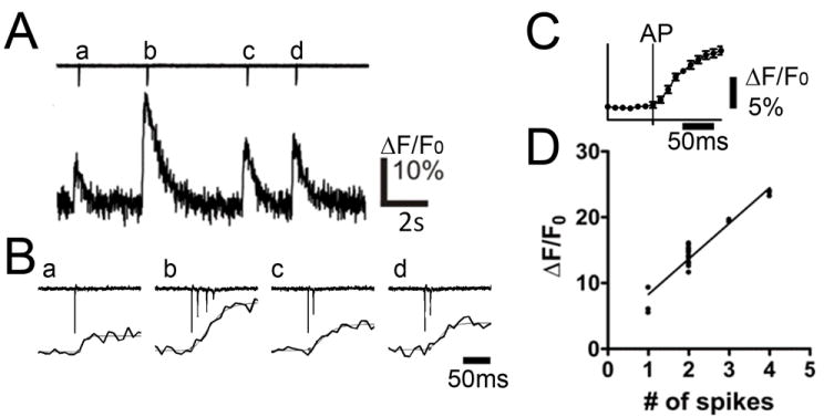
(A) Simultaneous loose patch recording (top) and change in fluorescence intensity (ΔF/F₀; bottom recorded from a spontaneously firing neuron. (B) Loose patch and calcium indicator fluorescence traces at higher temporal resolution. Note the close linkage between action potential firing (downward deflections in loose patch recording) and onset of calcium indicator response. (C) Plot of calcium indicator response relative to action potential firing (vertical line) derived from simultaneous whole cell patch and calcium indictor imaging. Note the tight relationship between the indicator response and cell firing. (D) Correlation between peak ΔF/F₀ value and number of action potentials in neuronal activity recorded from multiple neurons. (n = 3, Pearson r=0.956, p < 0.0001)

Spontaneous Synchronous Network Bursts

In most slices prepared from animals aged P4 to P6 (15 slices from 11 animals), we observed spontaneous synchronous activity in area CA3. A representative recording from a slice prepared from a P5 rat is shown in Fig. 2. Fig. 2B shows normalized fluorescence traces (ΔF/F₀) for 10 cells, along with a raster plot for 64 cells (out of 87) that participated in synchronous network activity. Based on the response of these bursts to application of GABA receptor antagonist (described in a later section), the frequency of events, and the animal age dependence of occurrence of these events, these network bursts fit the experimental definition of giant depolarizing potential (GDPs)(Khazipov et al., 1997; Sipila et al., 2005; Ben-Ari et al., 2007). As is evident in Fig. 2, the GDP events occurred repeatedly, i.e., four times in one minute. There was also occasional, intermittent non-synchronous activity independent from the synchronous events in a proportion of neurons. In this particular data set, 58 of 76 cells (76%) had no activity between synchronous events, and 16 of 76 cells (21%) exhibited isolated firing between synchronous events. The amplitude, or peak fluorescence value, of these non-synchronous events was often smaller than that seen during the synchronous events. Taken together with the fact that the ΔF/F₀ peak values of most cells during the synchronous events were ~40% (ΔF/F₀), and the fact that the 40% fluorescence response corresponds to multiple number of spikes in Fig. 1D, this suggests that neurons fired a burst of APs, i.e., multiple spikes, during synchronous spontaneous network events (also evident in Fig. 1).

Fig. 2. Spontaneous network bursts and onset time analysis.

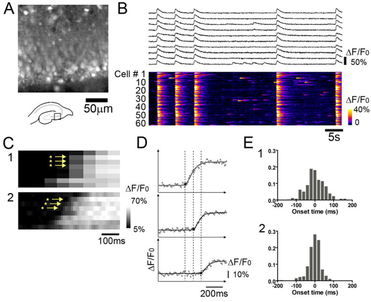
(A) An area CA3 steady state fluorescence (F₀) image obtained by fast confocal microscopy of an immature hippocampal slice stained with the calcium indicator OGB-1 AM. (B) Synchronous network activity recorded from area CA3. Normalized fluorescence changes (ΔF/F₀) traces for 10 cells (top) and raster plot of color-coded fluorescence vs. time (bottom) for 64 cells that exhibited synchronous network activity. The synchronous spontaneous network events occurred repeatedly. Note that there is non-synchronous isolated activity between the synchronous events. (C) Comparison of the utility of various image acquisition speeds in capturing neuronal activation onset times during spontaneous network bursts. ΔF/F₀ raster plots of grayscale-coded fluorescence change vs. time for 8 neurons that exhibited spontaneous synchronous activity. Images were captured at (1) 70 ms per frame, a typical speed with full frame (512×512 pixel) resolution, and (2) 11.2 ms per frame, the maximum speed that can be achieved by 4×4 binning with our EM-CCD camera. The faster acquisition speed was required to resolve differences in onset times among cells. (D) ΔF/F₀ traces (dots) for 3 different cells within a synchronous network event, together with an onset time estimation by sigmoid curve fitting (line). Dotted vertical lines depict differences in calculated cell onset times for the 3 neurons. (E) (1) Cellular onset latency distribution of spontaneous network bursts (4 bursts). Median onset time within a network burst was defined as zero. If a cell activated earlier than median value, negative values were assigned to the cell, while positive onset value was assigned to the cells that activated later than median timing. The majority of cells distributed within ~200 ms, with a standard deviation of 54 ms. (2) Cellular onset latency distribution of evoked synchronous events for the same cells shown in E1. The distribution became narrower, with the majority of cells responding within ~150 ms, with a standard deviation of 35 ms.

Sufficiently fast acquisition speeds were necessary to measure biologically relevant differences in individual cellular burst onset times during GDP events. In order to determine the minimal required temporal resolution to capture salient differences in cellular burst onset times, we imaged spontaneous GDPs at two different acquisition speeds; 70 ms per frame, a typical scanning speed for calcium imaging with high spatial resolution (Sasaki et al., 2006; Allene et al., 2008; Sasaki et al., 2008; Allene and Cossart, 2010) and 11 ms per frame, the maximum speed that could be obtained through 4×4 binning of the 512×512 pixel EM-CCD camera. Figure 2C shows temporal raster plots of several ROIs from two movies of spontaneous bursts recorded from a slice. The raster plot was zoomed and focused on the rising phase of signal change for a single network burst at both temporal resolutions. Although the two bursts may not be identical, the raster plot in Fig. 2C2 resolves differences in cellular burst onset timing to a much greater extent than the recording in Fig. 2C1. This demonstrated the requirement for higher temporal resolution recordings to resolve differences in cellular burst latencies underlying spontaneous GDPs.

Onset Time Distribution

For a series of images taken from the slice, the onset time of synchronous activity was estimated for each ROI (i.e., cell body) by fitting a sigmoidal curve to the rising phase of fluorescence change (see method section). Fig. 2D shows an example of onset time estimation for 3 different cells during a synchronous network event. The sigmoid curves fit the data well. Among 87 cells marked on the image, 15 cells had no synchronous responses and were excluded from the analysis. In addition, several cells had very small responses (less than 5% ΔF/F₀) and the rising phase of these responses was poorly fit (R² of less than 0.6). These cells were also excluded from further analysis. After determining the onset time for cells that resulted in a good fit (typically 63-65 cells), as a temporal reference point, the median onset time for the cell population was defined as zero. Cells activating earlier than the median were assigned negative onset time values, while cells which activated later than the median were assigned positive onset times.

Figure 2E1 shows the distribution of onset times for four spontaneous network events recorded from the same slice. As a control experiment, using the same slice, a stimulating electrode was placed in the Schaffer collateral pathway, away from the imaged area, and a burst stimulus (4 pulses, 10 μs, 100Hz, 500 μA) was applied. The electrical stimulus evoked a synchronous network event, and Figure 2E2 shows the onset time distribution of this response. For the spontaneous bursts, onset times ranged from -190 to +286 ms, with a standard deviation of 54 ms. In contrast, for the evoked bursts, the onset time ranged from -207 to +85 ms, with a standard deviation of 35 ms. This suggests that electrical stimulation triggered a different type of network activity, distinct from spontaneous events.

Burst Propagation

Since the CA3 layer was tilted slightly to the CCD camera field of view, we rotated the image during analysis to visually align the hippocampal axis, and new image axes were defined as x’ and y’ as shown in Fig 3. Figure 3A shows onset latency as a color-coded 2-dimensional map of cell location and cellular burst onset time for a spontaneous network burst. Warmer colors (red) indicate that cells activated earlier than the population median, and cooler colors (blue) indicate that cells activated later. In Fig. 3A, red circles (corresponding to cellular ROIs) predominate on the right side of the field, while blue ROIs are located mainly to the left, indicating that cellular activation propagated from right to left, or from CA3b to CA3c, as illustrated in the inset. This can be more clearly visualized by plotting the onset time relative to the cellular x’ location in a scatter graph (Fig. 2, bottom plots). Regression analysis of the cell location versus onset time plot facilitated determination of the direction of burst propagation within the network. In the example in Fig. 3A, the fitted latency curve had a minimum on the right side of the image, and the burst took ~140 ms to travel across the image, thus the propagation speed was estimated to be ~1.4 mm/s. Note that the burst propagation appeared non-linear, and that the larger slope in the fitted curve indicates slower traveling speed.

Fig. 3. Cellular activation onset analysis of propagation of spontaneous network bursts.

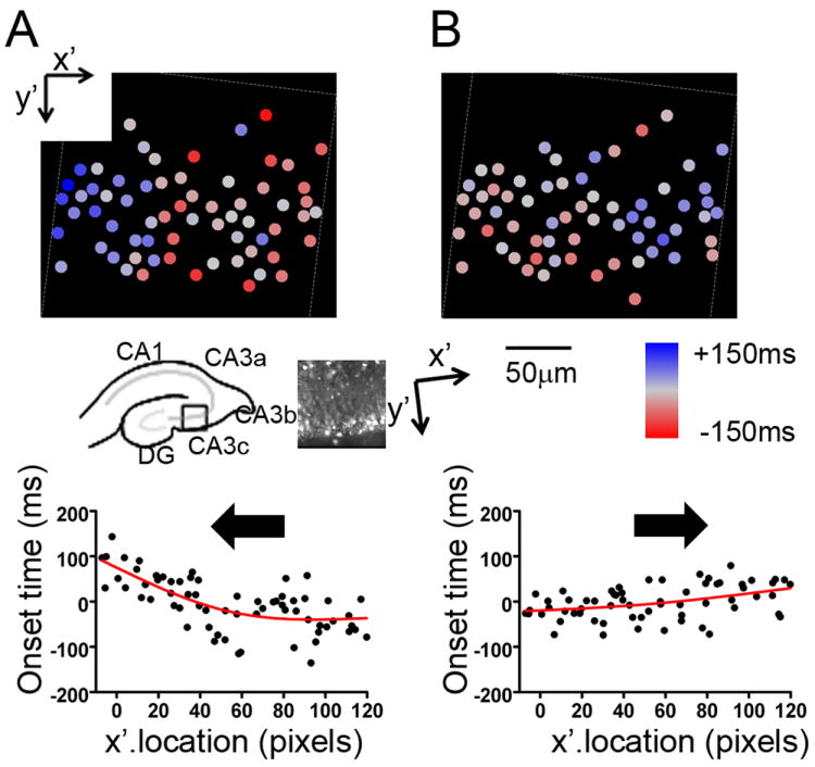
(A) (top) Color-coded cellular onset time mapping for a spontaneous GDP. Red color indicates that cells are activated earlier than the median timing and blue color indicates cells which activated later. Note that, for this burst, red ROIs are located more to the right side while blue ROIs are located mainly to the left, consistent with propagation from right to left (arrow in lower plot), or from CA3b to CA3c as illustrated in the inset. Note that since the CA3 layer was tilted slightly to the CCD camera field of view, the image was rotated to visually align the hippocampal axis, and new image axes were defined as x’ and y’ as shown in the inset. (bottom) Propagation effect can be seen more clearly by plotting x’-pixel location and onset time in a scatter graph, together with a regression line. (B) (top) Onset time plot for a different spontaneous event in the same region. Note that red ROIs are located more to the left side for this burst, consistent with event propagation from left to right (arrow in lower plot). (bottom) x’-pixel location/onset time scatter plot for this second burst. Note the opposite propagation direction. See Table1 for different types of network burst patterns observed in the same slice.

Figure 3B depicts the same analysis method applied to another spontaneous network burst in the same slice. For this burst, red ROIs are concentrated on the left side of the image, while the right side is dominated by blue ROIs, indicating the burst propagated from left to right, the opposite direction of the burst depicted in Fig. 3A. Here the burst travelled in an approximately linear fashion, with a slope of 50 ms per 128 pixels, translating to a speed of ~4 mm per second. Pearson’s correlation analysis between Y’ location and onset time resulted in no significant correlation.

In multiple recordings from the slice, we observed a total of 17 spontaneous and 12 evoked network bursts. Based on their characteristics of propagation, we assigned these events to several categories (Table 1). Spontaneous bursts with a slow propagation from right to left (CA3b to CA3c), as depicted in Fig 3A were seen in the majority of cases (14/17 events), and defined as a type I burst. A spontaneous burst with faster propagation from left to right (CA3c to CA3b), shown in Fig 3B, was seen only once, and was defined as a type II burst. A third burst pattern started in the center of the image and spread laterally in both directions (one event, Type III), and lastly we also observed a disorganized widely distributed onset (one event, Type IV). Evoked bursts propagated too quickly to resolve directionality, and were classified as Type V bursts.

Table 1.

Network Burst Patterns Observed in a Slice.

I	Propagation from Right to left (CA3b → CA3c)	14 out of 17 bursts
II	Propagation from Left to right (CA3c → CA3b)	1 out of 17 bursts
III	Propagation starts from the center	1 out of 17 bursts
IV	Disorganized	1 out of 17 bursts	ranges ~ 900ms
V	Evoked	12 observations	no directionality

Network bursts observed in a slice were categorized into several groups based on their onset time distributions and propagation characteristics.

Temporal Patterns Independent of Propagation

To begin to resolve additional sources of burst latency variation, we minimized contributions of burst propagation to onset times by restricting our examination to 10 closely neighboring neurons, comparing cellular burst latencies within this CA3 microcompartment. Fig. 4A depicts the 10 sampled neurons analyzed, Fig. 4B plots fluorescence traces for two representative network bursts in these cells. Table 2 lists onset time and ranks within these 10 cells for each burst. Based on analysis of burst onset latencies in this anatomically restricted area, cellular activation did not appear to be random. Instead, cells retained a consistent order of activation from burst to burst. Cell 4 repeatedly activated earlier than other cells, while cells 5, 6, and 7 consistently activated later than the majority of cells. To analyze this further, we ranked cells based on relative activation order (shown in Table 2) and the non-parametric ranking order statistic, Kendall’s W value, was calculated. Kendall’s W is an indicator of ranking order consistency. For these 10 cells and 9 network bursts, Kendall’s W was calculated to be 0.63, consistent with a highly repeatable activation order, which was extremely unlikely to occur by chance if activation was based on purely random ordering (p<0.0001). Based on their activation latencies, we termed cell 4 as an early responder and cells 5, 6, and 7 as followers.

Fig. 4. Temporal activation patterns independent of propagation characteristics.

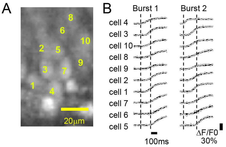
Onset time analysis for 10 closely-localized neurons, for 9 spontaneous GDPs that exhibited similar propagation patterns (Type I in Table 1). (A) Fluorescence image with cell i.d. number. (B) Fluorescence traces (ΔF/F₀) for 10 specified cells for two Type I bursts. The traces were ordered, earliest to latest, by the average latency of firing onset during the 9 bursts.

Table 2.

Onset Time (and Rank) for 10 closely located cells during GDPs.

Cell i.d.	Burst 1	Burst 2	Burst 3	Burst 4	Burst 5	Burst 6	Burst 7	Burst 8	Burst 9	Rank
1	18.5(7)	-13.3(6)	11.2(7)	-11.2(4)	-10.0(6)	-10.1(5)	13.4(7)	-0.6(5)	5.6(7)	6
2	44.0(8)	0.0(7)	-15.7(6)	-3.4(6)	10.3(8)	-7.8(7)	7.8(6)	0.6(6)	-51.5(2)	7
3	-14.1(5)	-18.1(4)	-19.0(5)	-31.4(2)	-42.9(2)	-28.0(4)	-21.3(3)	-26.3(1)	-50.4(3)	2
4	-56.9(3)	-87.0(1)	-105.3(1)	-53.8(1)	-101.5(1)	-100.8(1)	-35.8(1)	1.7(7)	-93.0(1)	1
5	65.3(10)	45.7(9)	84.0(10)	77.3(10)	76.2(10)	66.1(9)	49.3(9)	45.4(9)	54.9(9)	10
6	15.1(6)	63.8(10)	29.1(9)	29.1(8)	4.7(7)	86.2(10)	97.4(10)	86.8(10)	38.1(8)	9
7	47.6(9)	20.2(8)	25.8(8)	71.7(9)	23.4(9)	62.7(8)	17.9(8)	30.8(8)	57.1(10)	8
8	-56.8(4)	-22.5(3)	-39.2(2)	-11.2(5)	-26.4(3)	-9.0(6)	-29.1(2)	-25.2(2)	-32.5(6)	4
9	-87.9(1)	-15.9(5)	-31.4(3)	2.2(7)	-18.1(4)	-30.2(3)	-10.1(4)	-3.9(3)	-50.4(4)	5
10	-73.7(2)	-39.4(2)	-26.9(4)	-22.4(3)	-11.8(5)	-34.7(2)	-10.1(5)	-2.8(4)	-41.4(5)	3

Onset time in milliseconds for 10 cells for 9 GDP bursts shown in Fig 4. Ranks were defined as the earliest being 1^st and the latest 10^th. Overall ranks were calculated by sum of ranks across 9 bursts and smallest being defined as the 1^st. Note that cell 4 is repeatedly ranked 1^st and cell 5, 6, and 7 were always among the bottom 3.

Based on the above microcompartment analysis, we hypothesized that burst firing order was nonrandom irrespective of cellular location (i.e., burst propagation effects), and that individual neurons played distinct roles in defining burst structure (e.g. early responders and followers). To test this hypothesis further, we reexamined our data derived from larger fields, and minimized contributions of burst propagation to assess whether deterministic burst structures were evident in this larger area of the CA3 circuit. We first reanalyzed scatter plots (e.g. Fig. 3) for multiple bursts and determined if individual cells appeared consistently above or below the best fit regression line. If there was a consistent trend that a particular cell fired earlier or later than the timing expected from the propagating characteristic (regression line), this would support the hypothesis that burst structures are deterministic. We minimized the effect of cell location by examining residuals from the spline fit. We then calculated a correlation matrix of these residuals for 9 bursts. The median of Pearson’s r for all possible 36 pairs was 0.466, and ranged from 0.197 to 0.651 (all but one pair had significant correlation). This suggested that a consistent cellular activation order was retained, even after location factors were minimized.

Further evidence of deterministic burst structure was observed when comparing the waves that propagated in opposite directions as described in Fig. 3A and B. Pearson’s correlation of onset times between two bursts that propagated in opposite directions (i.e., Fig 3A &3B) was not significant. However, the correlation of residuals from the spline curves between the two bursts was 0.328 (p=0.013*). This emergence of a correlation between distinct burst types may be additional evidence of a temporal structure of bursts independent of burst propagation contributions.

Latent Class Analysis

Correlation analysis of residuals from the spline fittings (described in the previous section), provides support for the existence of a deterministic spontaneous network burst structure. However, correlation by itself does not address the question of whether there are individual cells which are ‘early responders’ or ‘followers’, nor does this type of analysis evaluate the existence of such groups. To begin to identify contributions of individual neurons to burst structure, and establish a statistical framework with which to evaluate the existence of classes (groups) of neurons with differing roles in burst firing order, we applied a latent class (LC) model, or finite mixture analysis, to explore the clustering of onset time (or onset time residuals) with the specific goal of determining whether there appeared to be a group (class) of neurons that represent early and/or late responders. Details of the LC analysis are discussed in the method section. Briefly, we fit LC models to the onset times by adjusting the effects of location using a spline. These models allow different numbers of underlying classes (groups) in the data where the membership of each observation to a particular class is unknown and estimated by the procedure. Each model fit to the data differed in the number of classes of cells it assumed. The best fit model or the best number of classes was chosen based on the minimum of an adjBIC.

Figure 5A shows a schematic illustration of the LC model analysis conducted on our data set. Specifically, onset time was fit to a spline curve in a class-specific manner by only shifting the offset, but not changing the spline function among the classes. By varying the number of classes (from 1 to 7) and the degrees of freedom for the spline fit (from 1 to 5), adjBIC were calculated for each scenario and the scenario expressing the minimum adjBIC value was selected as the optimum model. For our data set, this procedure identified 3 classes with a spline of degree of freedom of 5 as the best-fitting latent class model; adjBIC for df=5 (3187.5 (1 class)> 3182.2 (2 classes)> 3178.4 (3 classes) < 3183.4 (4 classes) < 3183.4 (5 classes)). The 3 classes were arbitrarily defined as ‘Early’, “Middle’, and ‘Late’, referring to the offset of the curve fitting. LC model analysis not only determines the number of latent classes but estimates the posterior probability for each cell belonging to each of the classes. Fig. 5B shows the posterior probability of 10 cells as members of three classes shown in bar graphs. For example, cell 1 in Fig. 5B had ~80% chance of being a member of the ‘Early’ class, and ~20% chance of being a member of the ‘Middle’ class. Cell 3 had a high chance of belonging to the ‘Middle’ class. Cell 4, had chances of being a member of the ‘Early’ (60%) or ‘Middle’(40%) classes. Thus, class assignment was made based on maximum posterior probability for a cell, with the magnitude of the probability indicating the confidence with which cells were assigned to a class.

Fig 5. Latent Class model analysis of cell activation latencies during bursts.

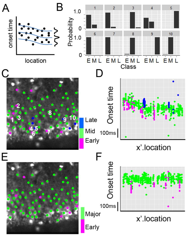
(A) Schematic illustration of LC analysis with class specific linear mixed model. Onset time was fit to class-specific spline curves without changing the shape but shifting intercept in a class specific manner. Vertical bell-shaped distributions at the right end of each line are class specific Gaussian distributions. LC analysis was conducted for different number of classes (from 1 to 6) and adjusted Bayesian Information Criteria (adjBIC) were calculated for each scenario and the scenario expressing the minimum adjBIC was selected as the optimum number of classes. LC analysis found 3 classes as the best-fitting model for GDPs. (B) Bar graphs of posterior probability of class membership for 10 representative cells (location shown in C) for the 3 class model, with E (Early Group), M (Middle Group), and L (Late Group). Cells were then assigned to a particular class based on their maximum posterior probability. (C) Color coded class assignment (Early red; Middle green; Late blue) superimposed on the image with the label for 10 cells show in (B). (D) Scatter plots of onset time vs. x’ location for all cells for 9 Type I burst responses with the class assignment in color (code as in C). (E) LC analysis of evoked bursts. Note that different groups of cells comprise the Early group for evoked bursts compared to spontaneous GDP bursts (C). (F) Scatter plots of onset times vs. x’ location for all cells for 9 evoked bursts with class assignment in color (Early red; Major green).

Table 3 shows a summary of the LC model analysis and class assignments with the mean response time indicating the difference between the classes. Of 76 cells analyzed, 10 cells (13%) were assigned to the ‘Early’ class, of which 5 cells were assigned with high probability (>90%, 6.5% of total cells). Six cells were assigned to the ‘Late’ class, with the majority of the cells (60 cells) assigned to the ‘Middle’ class. Figure 5C depicts a color-coded class assignment superimposed on the fluorescence image, together with the labeling for 10 cells shown in Fig. 5B. Comparing this to Fig. 4, the early responders cell 3 and cell 4 in Fig. 4 belong to the ‘Early’ group (cell 4 and 6 in Fig. 5C), and, similarly, the followers (cells 5, 6, and 7) belong to the ‘Late’ group in LC analysis. Finally, Figure 5D shows scatter plots of onset time for all cells for all 9 bursts, with color indicating class assignment. This plot clearly demonstrates that LC analysis is a powerful method for assigning cell classes, considering location factor. The data presented here and above is a representative data set, containing cells in the early responder group. We have applied a similar LC analysis to spontaneous GDPs from 4 other slices and found a comparable distribution of ‘early responder’ cells to that depicted in Fig 5 and Table 3. In total, 5.5±1% of cells (11/199 cells from 4 animals) were recognized as ‘early responders’ with high posterior probability (>90%) of class membership by LC analysis.

Table 3.

Class assignment by Latent Class (LC) analysis – GDPs and Evoked Bursts

Group	Mean (SE) 1 (ms)	Number of Cells (% of total) Assigned to Class 2	Number (% of Class) Assigned with High Probability 3
GDPs
Early	-45.0(11.1)	10(13%)	5(50%)
Middle	0(11.2)	60(79%)	56(93%)
Late	+116(13.3)	6(8%)	5(83%)
Evoked Bursts
Early	-80.9(28.5)	7(9%)	3(43%)
Majority	0(5.15)	68(91%)	62(91%)

¹offset in Middle class was defined as 0.

²based on maximum posterior probability across all classes

³based on maximum posterior probability of at least 0.90;

LC model analysis found 3 classes as the best fit model for GDPs. Mean values was obtained from the intercept of the class specific spline curve, with the standard deviation indicating the distribution (variability) of each class. We arbitrarily named these three classes as Early, Middle, and Late, based on the mean value. Class assignment was conducted based on maximum posterior probability for membership of each cell to each class (examples of posterior probability presented in Fig.5B). Of 76 cells analyzed, 10 cells were assigned to the ‘Early’ class, of which 5 cells were assigned with high probability. Six cells were assigned to the ‘Late’ class, with the majority of the cells (60 cells) assigned to the ‘Middle’ class. For evoked bursts, LC model analysis found 2 classes as the best fit model. We arbitrarily named the two classes as Early and Majority, based on the mean value. Among 75 cells, 7 cells were assigned to Early class (3 cells with high probability).

Temporal Patterns of Evoked Bursts

We also conducted a LC analysis on the network bursts evoked by electrical stimulation (Fig.2E2 and Type V in Table 1). The onset time distribution of evoked bursts was narrower than that seen for spontaneous events, as shown in Fig. 2E2, and the scatter plots for onset time vs x-pixel location had a best fitting spline (df=1) with a slope that was not different from 0. This suggested that the propagation speed of these evoked bursts was too fast to be captured and/or the propagation effect was swamped by large variance in the onset times. The correlation between repeated evoked burst measurements (9 bursts) on the same cells from different events ranged from 0.306 and 0.789, with a mean Pearson’s r for all pairs of 0.55 (all significant correlations). Thus, the correlation among repeated measurements collected for the same cell was substantial, which suggests that there is a consistent neuronal firing order, i.e, deterministic burst structure, even in the evoked bursts. The LC model analysis for these evoked bursts (N=9) generated two classes as the best fit model. The means and standard deviations of onset times for the two classes are shown in Table 4. We termed the two classes as ‘Early’ and ‘Major’. All but seven of the cells were assigned to the ‘Major’ class. Seven cells were assigned to the ‘Early’ class and, of these, four were assigned with high probability (>90%, Table 4). Figure 5F shows the scatter plot for each cell for 9 evoked bursts with class assignment in color. As with the first data set (spontaneous bursts), the minority class appeared to represent a distinct group based on the difference in the mean values, consistent with the notion of a distinct group of early bursters. Figure 5E depicts a color coded mapping of class assignment. When compared to the assignment in Fig. 5C for spontaneous bursts, it is evident that electrical stimulation triggers network bursts through a different activation pathway, and also that different groups of cells made up the early responder cohort of neurons for these two different bursts, even though they occurred in the same network of cells.

Table 4.

Class assignment by Latent Class (LC) analysis – Interictal Bursts.

Group	Mean (SE) 1(ms)	Number of Cells (% of total) Assigned to Class2	Number (% of Class) Assigned with High Probability3
Minority	-17.3(3.7)	3(7%)	2(67%)
Majority	0(1.4)	40(93%)	40(100%)

¹offset in Majority class was defined as 0.

²based on maximum posterior probability across all classes

³based on maximum posterior probability of at least 0.90

LC model analysis found 2 classes as the best fit model. We arbitrarily named the two classes as Minority and Majority. Class assignment was conducted based on maximum posterior probability of membership for each cell to each class. Among 43 cells, 3 cells were assigned to Minority class.

Effects of blockade of GABAergic Inhibition

GABAergic neurons play a crucial role in generation of network bursts in immature, early postnatal brains. In order to investigate the role of GABAergic neurons in generating and shaping the temporal characteristics of spontaneous synchronous bursts, the GABA_A receptor antagonist, bicuculline, was applied. There were distinct effects of bicuculline on spontaneous bursts recorded in rats and mice. In rats, application of bicuculline (10 μM) blocked the occurrence of spontaneous synchronous network events as shown in the raster scan in Fig. 6A (top, same slice prepared from a p5 rat was recorded in Figs 2-5). Note that the spontaneous isolated non-synchronous activity remained intact. The overall occurrence of non-synchronous activity remained similar before and after applying bicuculline (Fig. 2B vs Fig. 6A, top). Synchronous network bursts could still be evoked by electrical stimulation in the presence of bicuculline, as shown in Fig. 6A (bottom), with Fig. 6B showing a cumulative distribution of onset times in individual neurons. Interestingly, the onset time distribution for evoked events in bicuculline became wider (red) compared to the results obtained for spontaneous GDPs without bicuculline (blue, see also Fig. 2E). This suggests that GABAergic inhibition plays a role not only in the initiation, but also the shaping of synchronous network burst structure. In addition, the number of neurons that were activated by electrical stimulation was reduced in the presence of bicuculline (only ~50% cells responded to all 4 electrical stimuli). However, the phenomenon of deterministic activation order was maintained among the responding cells in bicuculline, as the average Pearson’s r for 4 bursts (6 pairs) was 0.613 (ranged from 0.509 to 0.771, all significant correlations).

Fig. 6. Effect blockade of GABAergic inhibition on burst characteristics – two distinct effects.

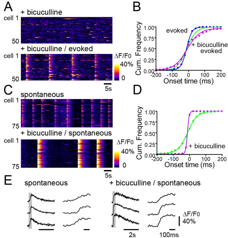
(A) Raster line scan plots of color-coded fluorescence intensity (ΔF/F₀) vs. time for 50 cells, in the presence of bicuculline (top) and during stimulation in the presence of bicuculline (bottom, 15 s intervals). Addition of bicuculline (10 μM) completely blocked GDP bursts; recorded from the same slice as shown in Fig 1-3, prepared from P5 rat. Note that bicuculline did not block non-synchronous activity and that synchronous bursts could still be induced by electrical stimulation. (B) Plot of onset time distribution for GDPs (green), evoked responses in the absence of bicuculline (blue), and evoked responses in the presence of bicuculline (red). Note that evoked responses without bicuculline exhibited a tighter, and bursts evoked in the presence of bicuculline a wider temporal distribution than GDPs. (C) Bicuculline did not block spontanous network bursts in every preparation. (top) Raster line scan plots of color-coded fluorescence intensity (ΔF/F₀) vs. time for 75 cells for spontaneous synchronous network bursts (P5 mouse), and (bottom) 10μM bicuculline did not block spontaneous network bursts but induced extremely synchronous and intense events. These network bursts were termed interictal bursts in the presence of bicuculline. (D) Plot of cellular activity onset time distribution of interictal bursts (purple dots) revealed cellular activation times were much tighter (30-40 ms window) than spontaneous bursts without bicuculline (green; 200-250 ms window). (E) Fluorescence traces(ΔF/F₀) from 3 representative cells in C. Spontaneous bursts (GDPs) on the left and spontaneous bursts under bicuculline (Interictal Bursts) on the right. Note that right traces in each panel are at an enhanced time scale. The intense interictal activity resulted in higher peak ΔF/F₀ values in individual neurons which decayed more slowly than that seen during GDPs. The rising-phase of ΔF/F₀ traces during interictal activity was also faster than that of GDPs.

Interictal Bursts

We observed synchronous network bursts that were completely blocked by bicuculline in many slices, particularly those prepared from rats. However, bicuculline did not always block spontaneous synchronous bursts. In 11 slices prepared from 7 mice, ages between P4 and P6, bicuculline application decreased the frequency of occurrence of spontaneous synchronous events, and increased the amplitude and intensity of these responses. This observation was also described by Le Magueresse and colleagues (Le Magueresse et al., 2006) who attributed this phenomenon to the emergence of epileptiform interictal discharges upon GABA blockade. Figure 6C illustrates this effect of bicuculline, depicting time raster plots of cellular fluorescence responses during spontaneous network bursts before (Fig.6C top) and after (Fig.6C bottom) addition of 10 μM bicuculline to a slice prepared from a P5 mouse. Interestingly, and in contrast to the evoked burst responses in bicuculline depicted in Fig.6A, the onset time distribution of bicuculline-transformed interictal activity was much tighter than that seen for spontaneous events before treatment (Fig. 6D), with all activation latencies falling within a range of three frames (33 ms), compared to >200 ms for control slices. The intense interictal activity resulted in higher peak ΔF/F₀ values in individual neurons (peak ΔF/F₀ up to 0.8) which decayed more slowly (~5 s) than that seen during GDPs (which exhibited a peak ΔF/F₀ up to 0.4 with a decay in ~2 s). The rising-phase of ΔF/F₀ traces during interictal activity was also faster than that of GDPs (Fig.6E).

In order to better resolve differences in cellular activation latency during this very tightly distributed interictal activity, we enhanced our imaging speed through use of a faster CCD camera, which allowed us to increase our image acquisition rate to 350 Hz. The onset time for interictal events varied within a range of 45 ms (16 frames at enhanced resolution) as shown in Fig. 7A. About 1/3 of cells had spontaneous non-synchronous runs of responses (not shown), which on occasion could occur immediately prior to a synchronous interictal burst, skewing the onset time analysis. In this dataset from 6 interictal bursts, 4 responses from 4 cells had responses up to 100 ms earlier than the majority of responses. Because this was not a repeatable occurrence in individual cells, and spontaneous responses could also occur not in association with network bursts, these 4 data points were discarded as outliers. This left responses from a total of 37 cells which had responses during all six waves. Correlations between repeated measures on the same cell from different bursts ranged from -0.26 to 0.55, with a median correlation of 0.06 (p value, not significant). Thus the correlations were substantially weaker than for the first dataset (Fig. 5). This indicates that interictal bursts exhibited a less deterministic burst structure than that seen during GDPs, associated with a more random neuronal activation order in repeated bursts.

Fig. 7. Interictal Bursts.

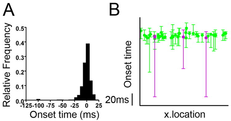
(A) Onset time distribution of interictal network bursts (imaged at 350 Hz). The cell activity latency clustered tightly (within ~40 ms), with 4 outlier values (arrows). (B) Latent class model analysis resulted in two classes as the best fit model. (see Table 4). Median onset time for each cell is plotted together with the range of values for 6 interictal bursts, with class assignment in color. The four most extreme negative outcomes in the dataset were outliers, and are evident in the wide range for one majority (green) and three minority (red) class cells. The median cell latency values for all cells overlapped.

To further examine this issue, we applied the latent class model to interictal burst discharges, using data from all 49 cells with a response to one or more of the six bursts, including the outliers discussed above. The latent class analysis identified 2 classes as the best fit model. Means and standard deviations for the two classes from the best-fitting latent class model are shown in Table 4. We termed the classes as ‘Minor’ and ‘Major’. All but three of the cells were assigned to the ‘Major’ class. Three cells were assigned to the ‘Minor’ class. Of these, 2 cells were assigned to the Minor class with high posterior probability (>90%). In contrast to the data in Fig. 5 derived for GDPs, the three cells in the ‘Minor’ class did not represent a distinct group, as median onset time for these cells were not different from cells in ‘Major’ class (Fig. 7B). Rather, each cell in the ‘Minor’ group had three out of the four most extreme negative outcomes in the multiburst dataset, i.e. outliers. These outliers appear to be highly influential in forcing the latent class model to have two groups. Thus while our analysis found two groups in these data, the results are much less consistent with the notion of a group of early responders. Our conclusion from this analysis is that interictal bursts exhibit little in the way of robust class structure, and therefore are comprised of a population of neurons exhibiting stochastic (non-ordered) firing latencies during synchronous network activation.

Discussion

GDP network bursts in CA3 are deterministic

In the present study, derived from a detailed microcircuit analysis, we found that there is a consistent, deterministic neuronal activation order underlying GDPs, which is distinct from the effects of cellular location or the propagation characteristics of these events. Statistical approaches demonstrating this phenomenon included a high correlation coefficient in neuronal firing latency from burst to burst after minimizing the cellular location factor, and distinct classes representing both early and late firing neuron populations in LC analysis. This contrasted with cell firing orders resolved during spontaneous interictal bursts, which appeared stochastic, with no cells repeatedly leading or lagging in firing latency during these events.

The spontaneous synchronous network bursts shown in Figs. 2-5 fit the characteristics of GDPs reported in the literature: they are observed in early postnatal ages, recur at repeated intervals, are sensitive to GABA_A receptor antagonists (bicuculline), and exhibit a broad temporal spread of neuronal activation timing (Ben-Ari et al., 2007). GABA operates primarily via chloride-permeable GABA_A receptor channels. During early development, neurons have a higher intracellular chloride concentration due to immature expression of transmembrane chloride transporters. Because of this, GABA triggers an efflux of chloride, membrane depolarization, summing in a net excitatory effect promoting AP firing. GDPs are generated by synergetic interactions between recurrent excitatory GABAergic and glutamatergic synapses, combined with intrinsic regenerative conductances of CA3 neurons (Khazipov et al., 1997; Sipila et al., 2005; Ben-Ari et al., 2007). Factors contributing to delayed action potential firing in CA3 neurons during GDPs have been subject to detailed analysis (Valeeva et al., 2010), where it was suggested that neuronal responses during GDPs were initiated by depolarizing IPSPs driven by GABAergic interneurons. These IPSP depolarizations were subthreshold for action potential firing. This required activation of persistent Na channels by the IPSP to further depolarize the neuron, which initiated delayed AP firing.

In our study, we found that neurons fired APs in a distribution spanning 200-300 ms during spontaneous GDP network bursts, even though, in many cases, these cells were close neighbors. Given that interneuron collaterals frequently distribute in intensely local arbors, this appears inconsistent with the contention that GABAergic interneuron activity alone can control the precise temporal activation order of multiple, adjacent pyramidal cells. Rather, we hypothesize that the activity of GABAergic neurons may control the global propagation direction, creating conditions amenable for pyramidal cells to fire APs, but the activation timing is determined by the distinct intrinsic properties, and perhaps anatomy, of the pyramidal cells (Ropireddy et al., 2011). We further hypothesize that the early, middle, or late class membership determined by the LC analysis is directly related to intrinsic, cellular properties such as transmembrane chloride gradients, resting membrane potential, and/or sodium or calcium channel activity. This may allow subsets of cells to respond more strongly (activate more readily) to smaller depolarizing inputs. We also speculate that class membership determined by the LC analysis could also be related to differences in synaptic connectivity or dendritic anatomy of individual pyramidal neurons. Neurons with more widely distributed dendrites may collect synaptic input (activity) from broader areas relative to a lesser neighbor, which could allow this cell to become a watchful early responder in wave propagation. Similarly, if a neuron has a more tightly distributed dendritic tree, it may be able to collect recurrent collaterals only from its own immediate neighbors, relegating this neuron to a follower role.

The fact that waves propagated in different directions within the same microcircuit (Fig. 3) suggests that there are numerous burst initiating locations within a slice. As depicted in Fig.5D, our analysis showed early responders were not necessarily the earliest activating cells within an image field, suggesting these early responders were not burst initiators. Because of their location (cell body layer) and cell body morphology (no larger than other cells) and the fact that we did not observe continuous firing in these early responders (which might be a characteristic of interneurons), we speculate these neurons are subsets of CA3 pyramidal cells. Early responders, once activated, could activate other principal neurons or interneurons through recurrent collaterals. Those secondary neurons could further activate other principal cells. Thus, it is possible that, without those early responders, GDPs may not propagate as effectively, nor recruit the same large proportion of neurons into the burst.

If the role of GDPs is to form functional connectivity by fire together-wire together mechanisms in developing hippocampal networks (Ben-Ari et al., 2007), the deterministic firing order we saw in our experiments (for example, Fig. 4) may have a significant role in forming temporally important wiring patterns. The fact that GDPs are so synchronous and activate such a large proportion of the network makes it unlikely that the GDP itself can carry cognitive information. However, the temporal patterns activated during the GDP may be important in future coding, where any two neurons that express associated temporal delays can carry important information in a temporal coding mechanism (VanRullen et al., 2005). It is also possible that the delayed activation in CA3 may have significant effects on downstream (CA1) signal transmission by delayed co-activation mechanisms. (Izhikevich and Hoppensteadt, 2009).

The importance of deterministic firing order in synchronous network bursts and the possible role of this phenomenon in neuronal coding has been examined previously (Beggs and Plenz, 2004). These investigators studied cultured cortical slices using a multi-electrode array, and analyzed network bursts. They also found several repeatable activation orders, albeit within a time scale of ~10 ms (compared to the 200-300 ms timescale of GDPs, Fig.4). In another multi-electrode array recording study from sensory cortex in vivo, population spikes caused by sensory stimuli as well as spontaneous events were analyzed (Luczak et al., 2009). These investigators also found a repeatable, sequential neuronal activation order that lasted ~100 ms. They argued that the patterns of activation order and frequency response comprised the ‘vocabulary’ of coding for sensory inputs.

Bicuculline-induced Interictal bursts are stochastic

Without the inhibitory synaptic transmission mediated by GABAergic neurons and possibly GABA release from mossy fibers (Safiulina et al., 2010), the CA3 network is mainly composed of glutamatergic excitatory principal cells and their recurrent collaterals. In contrast to GDPs, our experimental analyses could not identify any evidence for ordered burst structure (e.g. early or late responder groups) in interictal bursts occurring in the presence of bicuculline, seen exclusively in slices prepared from mice. Interictal bursts appear to be quite distinct from GDPs, implicating inhibitory synaptic transmission as critical both in the initiation and shaping of GDPs. Several studies have examined network burst generation mechanisms in disinhibited hippocampal networks (Miles and Wong, 1983; de la Prida et al., 2006; Jones et al., 2007). Using electrophysiology, de la Prida and colleagues demonstrated that initiation of spontaneous population bursts in disinhibited CA3 region followed a buildup of synaptic excitation and firing to a threshold level, which could take as long as 50 ms (de la Prida et al., 2006). This group also showed that activation of a single neuron could induce a network burst when the timing matched with the recovery period from the previous bursts (Jones et al., 2007, see also Miles and Wong, 1983), and furthermore, that ~50% of cells they investigated had the capability to induce a network burst, suggesting many cells could initiate buildup of cellular activity that lead to a population burst, supporting a stochastic process underlying burst generation. In our experiments, it is possible that the outliers we saw in Fig. 8B might correspond to a similar ‘buildup’ of activity. Since the cells that fired early did not retain this role repeatedly from burst to burst, we viewed the early firing phenomenon to be a stochastic process. The median onset time of these cells was not different from the remaining population (Fig. 8B), suggesting that the network was composed of a relatively homogenous population. This may be due to the fact that blocking interneuronal contributions to spontaneous network bursts created a much simpler network composed of only glutamatergic recurrent circuits.

Computational modeling studies examining mechanisms of network burst generation in homogeneous networks composed of only one cell type with varied connectivity and excitability parameters have found that a homogenous population could generate network bursts when cells have high connectivity and random wiring (Izhikevich, 2003). Additional modeling of neuronal avalanches showed that synchronous bursts were generated in noisy systems and did not require a self-organized, deterministic network (Benayoun et al., 2010). These modeling studies suggest that network bursts such as interictal activity in our experiments could be generated by stochastic mechanism without having a specific cell type that initiates these events.

In contrast to the above discussion on homogeneity, populations of ‘bursters’ have been found in area CA1 in the high K⁺ model of epilepsy as well as in tissue prepared from animal models of epilepsy (Jensen and Yaari, 1997; Sanabria et al., 2001; Becker et al., 2008; Chen et al., 2011). These investigators hypothesized that CA1 population bursts were generated by excitatory input from CA3 activating a ‘burster’ population in CA1 first, followed by these bursters recruiting regular pyramidal cells by local electrical field or local synaptic interactions. In area CA1 of brain slices prepared from epileptic animals, a significant proportion of cells (up to 47%) were found to be bursters, and activation of an individual burster neuron could trigger interictal events. The computational modeling study by Bogaard and colleagues also explored the role of heterogeneous populations on network bursts generation (Bogaard et al., 2009). When two types of bursting characteristics were mixed, only a small percentage (10%) of a bursting-favorable cell type could have a significant effect on network burst generation and its pattern. This complex burst generating mechanism, where heterogeneous populations (deterministic, defined by intrinsic properties of individual neurons) act on a stochastic process – a hybrid mechanism- may be the realistic model of actual bursting mechanism in epileptic brains.

References

- Allene C, Cossart R. Early NMDA receptor-driven waves of activity in the developing neocortex: physiological or pathological network oscillations? J Physiol-London. 2010;588:83–91. doi: 10.1113/jphysiol.2009.178798. [DOI] [PMC free article] [PubMed] [Google Scholar]
- Allene C, Cattani A, Ackman JB, Bonifazi P, Aniksztejn L, Ben-Ari Y, Cossart R. Sequential Generation of Two Distinct Synapse-Driven Network Patterns in Developing Neocortex. Journal of Neuroscience. 2008;28:12851–12863. doi: 10.1523/JNEUROSCI.3733-08.2008. [DOI] [PMC free article] [PubMed] [Google Scholar]
- Bastone LA, Putt ME, Ten Have TR, Cheung VG, Spielman RS. Genetic heterogeneity and trans regulators of gene expression. BMC Proc. 2007;1(Suppl 1):S80. doi: 10.1186/1753-6561-1-s1-s80. [DOI] [PMC free article] [PubMed] [Google Scholar]
- Becker AJ, Pitsch J, Sochivko D, Opitz T, Staniek M, Chen CC, Campbell KP, Schoch S, Yaari Y, Beck H. Transcriptional upregulation of Cav3.2 mediates epileptogenesis in the pilocarpine model of epilepsy. J Neurosci. 2008;28:13341–13353. doi: 10.1523/JNEUROSCI.1421-08.2008. [DOI] [PMC free article] [PubMed] [Google Scholar]
- Beggs JM, Plenz D. Neuronal avalanches are diverse and precise activity patterns that are stable for many hours in cortical slice cultures. Journal of Neuroscience. 2004;24:5216–5229. doi: 10.1523/JNEUROSCI.0540-04.2004. [DOI] [PMC free article] [PubMed] [Google Scholar]
- Ben-Ari Y, Gaiarsa JL, Tyzio R, Khazipov R. GABA: A pioneer transmitter that excites immature neurons and generates primitive oscillations. Physiological Reviews. 2007;87:1215–1284. doi: 10.1152/physrev.00017.2006. [DOI] [PubMed] [Google Scholar]
- Benayoun M, Cowan JD, van Drongelen W, Wallace E. Avalanches in a stochastic model of spiking neurons. Plos Comput Biol. 2010;6:e1000846. doi: 10.1371/journal.pcbi.1000846. [DOI] [PMC free article] [PubMed] [Google Scholar]
- Bogaard A, Parent J, Zochowski M, Booth V. Interaction of Cellular and Network Mechanisms in Spatiotemporal Pattern Formation in Neuronal Networks. Journal of Neuroscience. 2009;29:1677–1687. doi: 10.1523/JNEUROSCI.5218-08.2009. [DOI] [PMC free article] [PubMed] [Google Scholar]
- Bonifazi P, Goldin M, Picardo MA, Jorquera I, Cattani A, Bianconi G, Represa A, Ben-Ari Y, Cossart R. GABAergic Hub Neurons Orchestrate Synchrony in Developing Hippocampal Networks. Science. 2009;326:1419–1424. doi: 10.1126/science.1175509. [DOI] [PubMed] [Google Scholar]
- Carlson GC, Coulter DA. In vitro functional imaging in brain slices using fast voltage-sensitive dye imaging combined with whole-cell patch recording. Nature Protocols. 2008;3:249–255. doi: 10.1038/nprot.2007.539. [DOI] [PMC free article] [PubMed] [Google Scholar]
- Chen S, Su H, Yue C, Remy S, Royeck M, Sochivko D, Opitz T, Beck H, Yaari Y. An increase in persistent sodium current contributes to intrinsic neuronal bursting after status epilepticus. J Neurophysiol. 2011;105:117–129. doi: 10.1152/jn.00184.2010. [DOI] [PubMed] [Google Scholar]
- Cossart R, Lkegaya Y, Yuste R. Calcium imaging of cortical networks dynamics. Cell Calcium. 2005a;37:451–457. doi: 10.1016/j.ceca.2005.01.013. [DOI] [PubMed] [Google Scholar]
- Crepel V, Aronov D, Jorquera I, Represa A, Ben-Ari Y, Cossart R. A parturition-associated nonsynaptic coherent activity pattern in the developing hippocampus. Neuron. 2007;54:105–120. doi: 10.1016/j.neuron.2007.03.007. [DOI] [PubMed] [Google Scholar]
- de la Prida LM, Huberfeld G, Cohen I, Miles R. Threshold behavior in the initiation of hippocampal population bursts. Neuron. 2006;49:131–142. doi: 10.1016/j.neuron.2005.10.034. [DOI] [PubMed] [Google Scholar]
- Fellin T, Pascual O, Gobbo S, Pozzan T, Haydon PG, Carmignoto G. Neuronal synchrony mediated by astrocytic glutamate through activation of extrasynaptic NMDA receptors. Neuron. 2004;43:729–743. doi: 10.1016/j.neuron.2004.08.011. [DOI] [PubMed] [Google Scholar]
- Garaschuk O, Linn J, Eilers J, Konnerth A. Large-scale oscillatory calcium waves in the immature cortex. Nat Neurosci. 2000;3:452–459. doi: 10.1038/74823. [DOI] [PubMed] [Google Scholar]
- Hirase H, Qian LF, Bartho P, Buzsaki G. Calcium dynamics of cortical astrocytic networks in vivo. Plos Biology. 2004;2:494–499. doi: 10.1371/journal.pbio.0020096. [DOI] [PMC free article] [PubMed] [Google Scholar]
- Hofer SB, Ko H, Pichler B, Vogelstein J, Ros H, Zeng H, Lein E, Lesica NA, Mrsic-Flogel TD. Differential connectivity and response dynamics of excitatory and inhibitory neurons in visual cortex. Nat Neurosci. 2011;14:1045–1052. doi: 10.1038/nn.2876. [DOI] [PMC free article] [PubMed] [Google Scholar]
- Ikegaya Y, Aaron G, Cossart R, Aronov D, Lampl I, Ferster D, Yuste R. Synfire chains and cortical songs: temporal modules of cortical activity. Science. 2004;304:559–564. doi: 10.1126/science.1093173. [DOI] [PubMed] [Google Scholar]
- Izhikevich EM. Simple model of spiking neurons. Ieee T Neural Networ. 2003;14:1569–1572. doi: 10.1109/TNN.2003.820440. [DOI] [PubMed] [Google Scholar]
- Izhikevich EM, Hoppensteadt FC. Polychronous Wavefront Computations. Int J Bifurcat Chaos. 2009;19:1733–1739. [Google Scholar]
- Jensen MS, Yaari Y. Role of intrinsic burst firing, potassium accumulation, and electrical coupling in the elevated potassium model of hippocampal epilepsy. J Neurophysiol. 1997;77:1224–1233. doi: 10.1152/jn.1997.77.3.1224. [DOI] [PubMed] [Google Scholar]
- Jones J, Stubblefield EA, Benke TA, Staley KJ. Desynchronization of glutamate release prolongs synchronous CA3 network activity. J Neurophysiol. 2007;97:3812–3818. doi: 10.1152/jn.01310.2006. [DOI] [PubMed] [Google Scholar]
- Khazipov R, Leinekugel X, Khalilov I, Gaiarsa JL, BenAri Y. Synchronization of GABAergic interneuronal network in CA3 subfield of neonatal rat hippocampal slices. J Physiol-London. 1997;498:763–772. doi: 10.1113/jphysiol.1997.sp021900. [DOI] [PMC free article] [PubMed] [Google Scholar]
- Le Magueresse C, Safiulina V, Changeux JP, Cherubini E. Nicotinic modulation of network and synaptic transmission in the immature hippocampus investigated with genetically modified mice. J Physiol. 2006;576:533–546. doi: 10.1113/jphysiol.2006.117572. [DOI] [PMC free article] [PubMed] [Google Scholar]
- Luczak A, Bartho P, Harris KD. Spontaneous Events Outline the Realm of Possible Sensory Responses in Neocortical Populations. Neuron. 2009;62:413–425. doi: 10.1016/j.neuron.2009.03.014. [DOI] [PMC free article] [PubMed] [Google Scholar]
- Mammano F, Canepari M, Capello G, Ijaduola RB, Cunei A, Ying L, Fratnik F, Colavita A. An optical recording system based an a fast CCD sensor for biological imaging. Cell Calcium. 1999;25:115–123. doi: 10.1054/ceca.1998.0013. [DOI] [PubMed] [Google Scholar]
- McLachlan GJ, Bean RW, Peel D. A mixture model-based approach to the clustering of microarray expression data. Bioinformatics. 2002;18:413–422. doi: 10.1093/bioinformatics/18.3.413. [DOI] [PubMed] [Google Scholar]
- McLachlan G, Peel D. Wiley Series in Probability and Statistics. John Wiley & Sons; New York: 2000. Finite Mixture Models. [Google Scholar]
- Miles R, Wong RK. Single neurones can initiate synchronized population discharge in the hippocampus. Nature. 1983;306:371–373. doi: 10.1038/306371a0. [DOI] [PubMed] [Google Scholar]
- Ropireddy D, Scorcioni R, Lasher B, Buzsaki G, Ascoli GA. Axonal morphometry of hippocampal pyramidal neurons semi-automatically reconstructed after in vivo labeling in different CA3 locations. Brain Struct Funct. 2011;216:1–15. doi: 10.1007/s00429-010-0291-8. [DOI] [PMC free article] [PubMed] [Google Scholar]
- Rothschild G, Nelken I, Mizrahi A. Functional organization and population dynamics in the mouse primary auditory cortex. Nat Neurosci. 2010;13:353–360. doi: 10.1038/nn.2484. [DOI] [PubMed] [Google Scholar]
- Safiulina VF, Caiati MD, Sivakumaran S, Bisson G, Migliore M, Cherubini E. Control of GABA Release at Mossy Fiber-CA3 Connections in the Developing Hippocampus. Front Synaptic Neurosci. 2010;2:1. doi: 10.3389/neuro.19.001.2010. [DOI] [PMC free article] [PubMed] [Google Scholar]
- Sanabria ERC, Su HL, Yaari Y. Initiation of network bursts by Ca2+-dependent intrinsic bursting in the rat pilocarpine model of temporal lobe epilepsy. J Physiol-London. 2001;532:205–216. doi: 10.1111/j.1469-7793.2001.0205g.x. [DOI] [PMC free article] [PubMed] [Google Scholar]
- Sasaki T, Kimura R, Matsuki N, Ikegaya Y. Integrative spike dynamics of rat CA1 neurons: an in situ multineuronal imaging study. Neuroscience Research. 2006;55:S79–S79. doi: 10.1113/jphysiol.2006.108480. [DOI] [PMC free article] [PubMed] [Google Scholar]
- Sasaki T, Takahashi N, Matsuki N, Ikegaya Y. Fast and accurate detection of action potentials from somatic calcium fluctuations. J Neurophysiol. 2008;100:1668–1676. doi: 10.1152/jn.00084.2008. [DOI] [PubMed] [Google Scholar]
- Sasaki T, Minamisawa G, Takahashi N, Matsuki N, Ikegaya Y. Reverse optical trawling for synaptic connections in situ. J Neurophysiol. 2009;102:636–643. doi: 10.1152/jn.00012.2009. [DOI] [PubMed] [Google Scholar]
- Satten GA, Flanders WD, Yang Q. Accounting for unmeasured population substructure in case-control studies of genetic association using a novel latent-class model. Am J Hum Genet. 2001;68:466–477. doi: 10.1086/318195. [DOI] [PMC free article] [PubMed] [Google Scholar]
- Sipila ST, Huttu K, Soltesz I, Voipio J, Kaila K. Depolarizing GABA acts on intrinsically bursting pyramidal neurons to drive giant depolarizing potentials in the immature hippocampus. Journal of Neuroscience. 2005;25:5280–5289. doi: 10.1523/JNEUROSCI.0378-05.2005. [DOI] [PMC free article] [PubMed] [Google Scholar]
- Stosiek C, Garaschuk O, Holthoff K, Konnerth A. In vivo two-photon calcium imaging of neuronal networks. P Natl Acad Sci USA. 2003;100:7319–7324. doi: 10.1073/pnas.1232232100. [DOI] [PMC free article] [PubMed] [Google Scholar]
- Szatmary B, Izhikevich EM. Spike-Timing Theory of Working Memory. Plos Comput Biol. 2010;6 doi: 10.1371/journal.pcbi.1000879. [DOI] [PMC free article] [PubMed] [Google Scholar]
- Takahashi N, Sasaki T, Usami A, Matsuki N, Ikegaya Y. Watching neuronal circuit dynamics through functional multineuron calcium imaging (fMCI) Neuroscience Research. 2007;58:219–225. doi: 10.1016/j.neures.2007.03.001. [DOI] [PubMed] [Google Scholar]
- Valeeva G, Abdullin A, Tyzio R, Skorinkin A, Nikolski E, Ben-Ari Y, Khazipov R. Temporal coding at the immature depolarizing GABAergic synapse. Front Cell Neurosci. 2010;4 doi: 10.3389/fncel.2010.00017. [DOI] [PMC free article] [PubMed] [Google Scholar]
- VanRullen R, Guyonneau R, Thorpe SJ. Spike times make sense. Trends Neurosci. 2005;28:1–4. doi: 10.1016/j.tins.2004.10.010. [DOI] [PubMed] [Google Scholar]
- Vogelstein JT, Watson BO, Packer AM, Yuste R, Jedynak B, Paninski L. Spike Inference from Calcium Imaging Using Sequential Monte Carlo Methods. Biophys J. 2009;97:636–655. doi: 10.1016/j.bpj.2008.08.005. [DOI] [PMC free article] [PubMed] [Google Scholar]
- Yang TY. A tree-based model for homogeneous groupings of multinomials. Stat Med. 2005;24:3513–3522. doi: 10.1002/sim.2182. [DOI] [PubMed] [Google Scholar]
- Zwietering MH, Jongenburger I, Rombouts FM, Vantriet K. Modeling of the Bacterial-Growth Curve. Applied and Environmental Microbiology. 1990;56:1875–1881. doi: 10.1128/aem.56.6.1875-1881.1990. [DOI] [PMC free article] [PubMed] [Google Scholar]