An Integrated Framework for HARDI-based Investigation of Structural Connectivity

Abstract

Structural connectivity models hold great promise for expanding what is known about the ways information travels throughout the brain. The physiologic interpretability of structural connectivity models depends heavily on how the connections between regions are quantified. This paper presents an integrated structural connectivity framework designed around such an interpretation. The framework provides three measures to characterize the structural connectivity of a subject: 1) The structural connectivity matrix describing the proportion of connections between pairs of nodes, 2) The nodal connection distribution characterizing the proportion of connections that terminate in each node and 3) the connection density image which presents the density of connections as they traverse through white matter. Individually each possess different information concerning the structural connectivity of the individual and could potentially be useful for a variety of tasks, ranging from characterizing and localizing group differences, to identifying novel parcellations of the cortex. The efficiency of the proposed framework allows the determination of large structural connectivity networks, consisting of many small nodal regions, providing a more detailed description of a subject’s connectivity. The nodal connection distribution provides a grey matter contrast that can potentially aid in investigating local cytoarchitecture and connectivity. Similarly the connectivity density images offer insight into the white matter pathways, potentially identifying focal differences that affect a number of pathways. The reliability of these measures was established through a test/retest paradigm performed on 9 subjects while the utility of the method was evaluated through its applications to 20 diffusion datasets acquired from typically developing adolescents.

Introduction

The in-vivo mapping of structural brain connectivity is now routinely included in research studies investigating neurologic development (Hagmann, Sporns et al. 2010), as well as specific diseases such as attention deficit hyperactivity disorder (Konrad and Eickhoff 2010) and schizophrenia (Yu, Sui et al. 2011). This new analysis paradigm seeks to utilize fiber tracking algorithms and diffusion weighted MRI (DW-MRI), to elucidate the anatomical connections that exist between various brain regions.

With this goal in mind, there are two traits which could be expected from a structural connectivity framework. First, while DW-MRI possesses information concerning the orientation of the local WM anatomy, it cannot distinguish between afferent and efferent axonal fiber bundles. Thus the functional directionality of the axonal fiber bundles connecting two regions cannot be determined and one should expect a symmetric structural connectivity measure between any pair of regions (the measure from A to B should equal that from B to A). Secondly, the anatomical connections we would like to model, namely axons, originate and terminate from neurons located within the GM. While many of these are commissural or long association tracks, others are short range connections between regions within the same gyrus or neighboring gyri. Thus we would expect that contrast provided by the paths of the connections to be somewhat evenly balanced between the major central WM tracts and the more cortical WM.

The most prominent work on structural connectivity (Hagmann, Kurant et al. 2007; Hagmann, Cammoun et al. 2008; Zalesky, Fornito et al. 2010) rely on whole brain tractography to provide a single set of fiber streamlines that are used to represent the axonal fiber bundles of the brain. Connectivity weights between GM regions are determined by counting the number of streamlines whose endpoints lie within those regions, sometimes normalized by the length of the tracks. These streamlines can also be use to generate fiber or track density images (TDI) (Calamante, Tournier et al. 2010) providing a white matter contrast by counting the number of streamlines passing through each voxel. Thus both the track density images and the connectivity weights between GM nodes are descriptions of the same set of fiber tracks used to represent structural connectivity.

These methodologies, by using fiber streamlines as surrogate fiber bundles achieve the desired symmetry expected from a structural connectivity measure. However the use of every voxel, either white or grey matter, as fiber tracking seeds causes an oversampling of large central fiber bundles that traverse many voxels. In the process shorter U-fibers or association fibers are under sampled, which might be problematic for studies of pathologies such as autism that may require the investigation of short as well as long range connectivity.

Alternative approaches have been proposed that track directly from the GM nodal regions. (Robinson, Hammers et al. 2010) uses a probabilistic Monte-Carlo (MC) based fiber tracking (Behrens, Woolrich et al. 2003) strategy, where the paths of individual particles are tracked, to determine the connecting fibers between regions. (Gong, He et al. 2009; Gong, Rosa-Neto et al. 2009) use MC fiber tracking to compute the connection probability between two nodes. The inherent dependence on the seed region generates a non-symmetric connectivity measure which is also difficult to attribute a physiological meaning to.

Several approaches have been proposed that combine anisotropy measures with fiber tracking methods to produce a connection weight between nodes. In (Iturria-Medina, Canales-Rodríguez et al. 2007; Iturria-Medina, Sotero et al. 2008), the authors determine the most probable path connecting any two nodes. The connection weight is then determined as the lowest anisotropy along that path. Similarly (Robinson, Hammers et al. 2010) integrates anisotropy along MC generated paths yielding a connection weight. An additional confound of the MC based methods is the dependence on the number of particles used in the model. The use of smaller GM nodal regions necessitates an increased number of particles per region placing an additional computational burden on the model.

The goal of this work is to present a structural connectivity framework designed explicitly around the physiological constraints discussed above. This lends our framework a clear physiological interpretation, being proportional to the number of physical connections between regions, which may yield testable hypothesis about the underlying biology of the systems under investigation. The method utilizes a discrete stochastic tractography algorithm, similar to (Iglesias, Thompson et al. 2010), to model the transition of particles through the neuronal WM volume. The efficiency of this approach allows the investigation of large networks of small nodal regions yielding a more detailed description of a subject’s connectivity, while removing the dependence on the number of particles, as required for modeling by the MC techniques. Using the discrete stochastic tractography algorithm, we compute a conditional probability matrix relating the GM regions that serve as nodes in the structural connectivity network. The network nodes are defined along the boundary of the WM volume, avoiding the preferential sampling of larger fiber bundles achieved by seeding in WM voxels.

From the conditional probability matrix, we determine the nodal connection distribution (nCD), defined as the steady state distribution of particles terminating at each nodal region. The nCD is computed by an optimization framework incorporating physiologic constraints, namely the conservation of structural connections, as well as the expected symmetry of the final structural connectivity matrix. This provides an in vivo contrast for GM regions that may prove interesting in investigating pathologies which affect local connectivity and cytoarchitecture. The structural connectivity matrix is then computed by combining the nCD and the conditional probability matrix. This removes the conditional dependence on the seeding regions while imparting the connectivity measure with a physiological interpretation. Finally the nCD can be mapped back into the WM voxels yielding a WM connection density image whose contrast is based on the number of particles traversing each voxel. This image provides a means to investigate spatial differences in WM integrity and, perhaps, focal effects of pathology.

The repeatability of the proposed method is illustrated through a test/retest study, consisting of diffusion datasets acquired at two time points on 9 subjects. All three connectivity measures are characterized by high test-retest reliability as evidenced by high correlations between each time point. Additionally, the method is applied to diffusion datasets acquired on 20 typically developing adolescents between the ages of 10 and 15 years. A 2744 element volumetric parcellation of the GM was used to compute the nCD and connectivity matrix for each subject. The spatial distribution of the population average nCD shows a varying pattern of connection concentration, with a focus in the temporal lobe that is well conserved across the population. Similarly, the connection density images computed using this framework agree with physiological expectations concerning distribution of connection within the corpus callosum (Aboitiz, Scheibel et al. 1992; Highley, Esiri et al. 1999), and demonstrate that large central WM pathways and cortical WM regions are equally well characterized, which is important to the study of pathologies where local connectivity is thought to be affected.

Methods

We compute a probability distribution function at every voxel of a subject’s DW-MRI dataset, describing the orientation of the anatomical fibers. In this work, the normalized fiber orientation distribution (FOD) function (Anderson 2005; Tournier, Calamante et al. 2007) is used for this purpose, although other models could be used. From the FOD field and a parcellation of the brain indentifying the GM nodes and the WM voxels, we seek to determine a measure proportional to the number of physical connections between the GM nodes, culminating in the creation of the structural connectivity matrix. In doing so, two other connectivity features are also computed: the nodal connection distribution and the connection density image. These three elements, seen in Figure 1, possess different information concerning the structural connectivity of the individual and could potentially be useful for a variety of tasks, ranging from characterizing and localizing group differences, to identifying novel structural and functional parcellations of the cortex. The details of procedure are discussed below.

Figure 1.

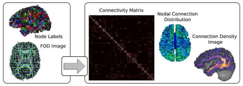
The framework utilizes a set of GM nodal regions and a fiber orientation distribution (FOD) image to determine three features related to the structural connectivity of the subject: 1) a structural connectivity matrix (only left hemisphere is shown) describing the number of connections between each pair of nodes, 2) the nodal connection distribution (nCD), describing the proportion of connections terminating in each node, and 3) a connection density image describing the density of connections as they traverse the WM.

Conditional Probability Matrix Computation

The first part of the framework is the computation of the conditional probability matrix (C). This matrix describes the likelihood that fibers terminate in a specific GM node, given that the other end is known to terminate in another GM node. This is accomplished by modeling the transport of particles assumed to travel along anatomical fiber pathways through the WM. The method determines each element, C_ij, as the proportion of particles injected into the system from the j^th node, that traverse the WM volume and exit into the i^th node. This approach shares the basic assumption of the MC fiber tracking approaches (Behrens, Woolrich et al. 2003; Gong, He et al. 2009), namely, that particles will travel along the underlying anatomical fibers. However, as opposed to modeling the transport of each particle individually, making the accuracy dependent on the total number of particles simulated, a Markov process is used to model the transport of a population of particles through the WM, allowing the conditional probability matrix to be efficiently computed.

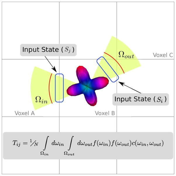
The efficiency of this approach derives from the discretization of the allowed states that particles traversing the WM volume can take. The collection of these states (S) make up the state space of the Markov process. A state is defined as a directed edge of the WM voxels (see Figure 2), and is, therefore, fully described by its base voxel and its target voxel. A state, S_j in Figure 2 for instance, representing particles moving from voxel A into voxel B, would have a base voxel A and target voxel B. In order to aid in determining feasible connections between states, each state is labeled based on the tissues types it connects. The available labels are WM-internal (WM to WM transitions), CSF-boundary (WM to CSF transitions), GM-out (WM to GM transitions) and GM-In (GM to WM transitions).

Figure 2.

States are defined as directed voxel edges. For instance S_j describes particles traveling from voxel A to B, while S_i describes those moving from voxel B to C. The transition probability between these states (T_ij) is defined by integrating the product of the FOD, at the intermediate voxel (voxel B) evaluated at the acceptance angle (ω_in ∈ Ω_out) and the outgoing angle (ω_in ∈ Ω_out) and a directional coupling term (c(ω_in, Ω_out)), which penalizes large turns.

For each voxel in the WM region, 26 states are formed, connecting the WM voxel to its 26 spatial neighbors. Each state is formed by the WM voxel acting as the base voxel and the neighboring voxel acting as the target voxel. These states are labeled as WM-internal, CSF-boundary, or GM-out based on the segmentation label of the target voxel. Once all the WM voxels and neighbors have been visited, we determine the GM-in states by inverting the base and target voxel of each GM-out states. The GM-in and GM-out states are then investigated to identify which GM nodes they are interacting with. This information is used to build two linear operators that map from the state space (S) to the space defined by the GM nodes (N). The first operator, B, describes the mapping from N to the incoming GM boundary states of S while the second operator, L, describes the mapping from the outgoing GM boundary states of S to the GM nodes. For instance, if g is a distribution of particles in the GM nodes (a vector in N), then Lg represents those particles entering into system’s state space. Similarly, if s is a distribution of particles in the state space, then Bs yields the number of particles that are transitioning into each of the GM nodes.

With the state space fully defined, we can describe how a distribution of particles (represented as a state vector) evolves in time. This evolution is governed by the transition matrix (T), where the ij^th element, T_ij, is the probability that particles in the j^th state will be in the i^th state at the next time point. Once T is defined, the dynamics of the system are expressed as s_t = T s_t−1, where s_t and s_{t −1} are state vectors at time step t and t−1, respectively.

The computation of each T_ij is made simpler by considering the tissue types connected by the first state. For instance, if S_j is a GM-out state, then its particles are leaving the WM system and not transitioning to other states, resulting in T_ij =0 for all possible S_i. Alternatively if S_j is either a WM-internal or GM-in state, then T_ij is computed only for situations, like those shown in Figure 2, where the transition from S_j to S_i represents a continuous trajectory, meaning that the base voxel of S_i is the target voxel of S_j. All other states have 0 transition probability.

Figure 2 demonstrates a case where the transition probability is non-zero. In this case, the transition probability is the likelihood that fibers travel from voxel A through voxel B and then into voxel C. The possible incoming particle trajectories connecting B and A are designated by the solid angle, Ω_in. Similarly Ω_out describes the possible exit trajectories into voxel C. Thus a possible trajectory through voxel B consists of a pair of incoming and outgoing directions, ω_in and ω_out. The likelihood that a particle would take that path through the voxel, is the product of the voxel B’s normalized FOD, f, evaluated at those two directions, multiplied by a coupling or inertia term that penalizes large turning angles. By integrating this product over the incoming and outgoing solid angles and normalizing by the integral over all possible directions, we arrive at the final transition probability connecting S_j to S_i

$$T_{ij}=1/N\underset{{\mathrm{\Omega }}_{in}}{\int }d{\omega }_{in}\underset{{\mathrm{\Omega }}_{\mathit{out}}}{\int }d{\omega }_{\mathit{out}}f({\omega }_{in})f({\omega }_{\mathit{out}})c({\omega }_{in},{\omega }_{\mathit{out}})$$ (1.1)

In this work, we choose c(•) to have the form of rejecting turns greater than 60 degrees, which has the desired result of greatly reducing particle deflections greater than 90 degrees. Other cutoffs are possible; however, preliminary results indicated that variations of up to 10 degrees had little effect on the final connectivity result. Finally, because physiologic fibers do not terminate in the CSF, we treat the CSF boundary as a particle sink by zeroing transition probabilities into states connecting WM and CSF voxels and then renormalizing the transition probabilities of those states.

With the dynamics of particle transport defined, the steady state behavior of the system under a constant input can be examined. Let b be a state vector describing a distribution of particles being injected into the system from the GM nodes. The dynamics of the system are captured by s_t+1 = T s_t + b, allowing for the computation of the equilibrium state vector (x) as

$$\begin{array}{l}x=Tx+b\\ x={(I-T)}^{-1}b\end{array}$$ (1.2)

This approach possesses a number of advantages over methods which track the progression of a single bolus of particles (Iglesias, Thompson et al. 2010). First, by utilizing the equilibrium behavior of the system as opposed to tracking an initial impulse of particles, this method is immune to geometries where particles exit the system very slowly, such as circular paths or loops. Secondly, while the matrix (I − T) is not easily invertible, due mainly to its high dimensionality, robust software tools (Balay, Gropp et al. 1997; Heroux, Bartlett et al. 2005) exist for efficiently solving such systems. Finally, this approach allows us to directly express a formula for the conditional connectivity matrix (C) relating the GM nodes as

$$C=L{(I-T)}^{-1}B$$ (1.3)

where B is used to map a distribution in the space of GM nodes into the state space, (I−T)⁻¹ determines the equilibrium behavior and finally, L maps the outgoing particles of the equilibrium state into their destined nodes. In this way, C_ij is the proportion of particles injected into the system from the j^th node that exit the WM volume into the i^th node and is equivalent to a conditional probability.

The algorithm used for computing C, solves for each column of C individually, essentially solving for the conditional connectivity of each GM node individually. The first step of this procedure is to compute an ILU precondtioner for the operator (I−T). Then for each column of B, we use an iterative solver to compute x = (I−T)⁻¹ B:_i. Both the preconditioner and the iterative solver are supplied as part of the Trilinos (Heroux, Bartlett et al. 2005) software package. Once x is determined, the corresponding column of C is filled with Lx. This approach can be fully parallelized, allowing for multiple columns of C to be determined simultaneously.

Nodal Connection Distribution and the Structural Connectivity Matrix

The columns of C describe the proportion of particles traveling from one node to another. For instance, if C_ij =0.25, then one quarter of the particles entering the WM from the j^th node, exit into the i^th node. Under the assumption that particle traffic between nodes is proportional to the number of anatomical connections between those nodes, it implies that ¼ of the connections that terminate at the j^th node have their other endpoint in the i^th node. If the distribution of connections across the GM nodes, the nodal connection distribution, is known, it can be combined with the conditional probability matrix (C) to compute a structural connectivity matrix, M, where each element is proportional to the number of connections between each pair of nodes.

$$\begin{array}{l}{M}_{:,i}=C_{:,i}{d}_i\\ M=CD\end{array}$$ (1.4)

where D is a diagonal matrix with the nodal connection distribution (d) along the diagonal.

The nodal connection density, d, is computed via an optimization problem that stipulates that the number of incoming connections from the other nodes must equal the number of connections outgoing from that node. As this may not lead to a unique solution, we also require that M, computed by equation 1.4, is symmetric. Thus d should obey the following relations

$$\begin{array}{l}d=Cd\\ M=M^t\end{array}$$ (1.5)

These constraints, combined with the non-negativity of d and the requirement that the elements of d sum to 1, form a convex quadratic optimization problem which is solved using the cvxopt (http://abel.ee.ucla.edu/cvxopt/) software package.

White Matter Connection Density Maps

Once the nodal connection distribution has been computed, the Markov model can be used to map those connections from the nodes back into the WM volume, generating an image displaying the concentration of connections as they traverse the WM. This is accomplished by using the steady state model to map the nCD (d) into the state space via

$$s={(I-T)}^{-1}Bd$$ (1.6)

The connection distribution in the state space, s, is then mapped into the image space using the base index of each state as the imaging voxel containing those connections, resulting in an image of the spatial distribution of connections throughout the WM volume called the connection density image (see Figure 1).

Results: Application to in-vivo HARDI datasets

In order to illustrate, characterize and compare the proposed methodology to existing techniques, as well as to test the replicability of the proposed measures, the framework was applied to two diffusion datasets. The first, designed to evaluate sensitivity and repeatability of the proposed method, consists of 9 subjects (2 Female/7 Male) with a mean age of 31.2 ± 4.2 years, imaged at two time points separated by two weeks. The second dataset is a population of 20 adolescent subjects (10 Female/10 Male) with a mean age of 11.9 ± 1.6 years. All participants were carefully screened to ensure that they did not have a history of current or prior neuropsychiatric symptomatology. Datasets acquired from all subjects were processed using the following processing pipeline.

Image Acquisition

For each subject a whole brain HARDI dataset was acquired using a Siemens 3T Verio^™ MRI scanner using a monopolar Stejskal-Tanner diffusion weighted spin-echo, echo-planar imaging sequence (TR/TE=14.7s/110ms, 2mm isotropic voxels, b=3000 s/mm², number of diffusion directions=64, 2 b0 images, scan time 18 minutes). A structural image was acquired, using an MP-RAGE imaging sequence (TR/TE/TI = 19s/2.54ms/.9s, 0.8mm in plane resolution, 0.9mm slice thickness) to facilitate tissue segmentation.

Processing

Prior to computing the FOD image from each subject’s DW-MRI image, a number of preprocessing steps were performed to reduce imaging artifacts and improve signal to noise. The DW-MRI images were first filtered using a joint linear minimum mean squared error filter to remove Rician noise (Tristán-Vega and Aja-Fernández 2010). This was followed by eddy current and motion correction, performed via the affine registration of each DW-MRI volume to the non diffusion-weighted (b0) image (Jezzard, Barnett et al. 1998). The FOD image for each subject was then computed using the constrained spherical deconvolution method (Tournier, Calamante et al. 2007). Nonlinear FOD based spatial normalization (Bloy, Ingalhalikar et al. 2011) was used to register each subject’s FOD to that of a 12 year old male subject which served as a population template. The registered FOD images where then normalized yielding an image of FODs, each with unit integral.

Within the template coordinate system, the template’s structural image was segmented into GM, WM, CSF using Freesurfer (Fischl, Sereno et al. 1999). A set of GM nodes was determined by downsampling the GM tissue segmentation to an isotropic resolution of 8mm. Each of these GM voxels were then given a unique label and then resampled at the native 2mm resolution. This yielded a set of 2744 unique GM nodes comprised of both cortical and sub-cortical regions. Additionally each GM node was assigned an anatomical label from the Desikan atlas (Desikan, Segonne et al. 2006). Using this set of 2744 GM nodes, a structural connectivity matrix, a node connection distribution and a connection density image were computed for each subject (as in Figure 1). In order to aid in visualization as well as comparability to published methods, the connectivity matrices were downsampled to the 86 anatomical nodes defined in the Desikan atlas. Each of the 2744 nodes corresponding to the same anatomical label, had its rows and columns summed to create a connectivity matrix in the coarser GM node space.

Repeatability Results

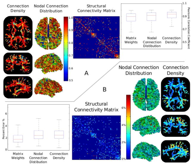
Two measures, Pearson’s correlation coefficient and the average percent error, were used to measure the reliability of each of the three measures of the proposed framework. For each WM voxel the connection densities at time point 1 were correlated to those at time point 2, yielding a correlation coefficient at every voxel. Similarly the values of the nodal connection distribution and of the weights of structural connectivity matrix can be used to generate correlation coefficients for each of these measures. These are shown in Figure 3A, along with a box plot illustrating the spread of these correlation coefficients. Similarly, Figure 3B, displays the percent error of these measures computed at each WM voxel, GM node and connectivity matrix weight. The percent error is computed as the difference between time point 1 and 2 divided by their mean. These results indicate that the majority of measures had correlation coefficients above 0.75 and errors below 5%.

Figure 3.

Results from a test/retest study performed on nine subjects scanned at two time points two weeks apart. Pearson’s correlation coefficients computed from each WM voxel’s connection density value, each GM node’s nodal distribution value, and each non-zero (p<0.025) connection weight, are shown in A. B shows the percent error of each of these measures. The high correlation coefficients, typically above 0.75, and low percent errors are indicative of a highly repeatable measure.

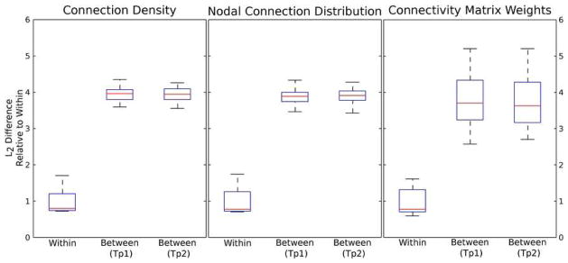
Additionally we were interested in the degree that each of these measures can be used to differentiate between subjects. For each measure, the difference between any two subjects was quantified using the L2 difference of the measures. Thus the difference between two subjects’ connection densities was computed as the square root of the sum squared difference in connection density of every WM voxel. Similarly the differences in nodal connection distribution (nCD) and structural connectivity matrix were computed as the square root of the sum squared difference of the nCD at every node and the difference of each non-zero connection weight respectively. Non-zero connection weights were determined by a student’s t-test thresholded at p < 0.025. Boxplots showing the average inter- and intra-subject differences for each of these measures are shown in Figure 4.

Figure 4.

Boxplots indicating the average L2 difference between connection density images, nodal distributions and connectivity matrices derived from the same subject (‘Within’) and different subjects at each time point (‘Between TP1 and TP2’). The average difference between subjects is roughly 4 times higher than the difference within the same subject, indicating that these measures are able to capture individual anatomy and may be able to reveal group differences.

Adolescent Population Results

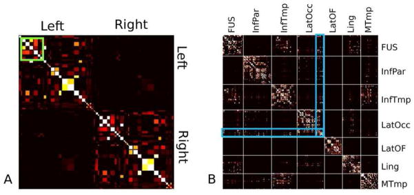
While the utilization of smaller nodal regions provides useful information (Figure 5B), the direct visualization and interpretation of entire structural connectivity network consisting of 2744 GM nodes is difficult. As many of the published works have been on smaller anatomically defined node definitions, we downsampled the connectivity matrices. Figure 5A shows the population average connectivity matrix downsampled to the 86 anatomical nodes chosen from the Desikan atlas. Figure 5B shows a portion of the higher resolution connectivity matrix for 7 anatomically defined nodes, highlighted in green, in Figure 5A.

Figure 5.

The average connectivity matrix (A), computed using the Desikan atlas. A large number of self connections are evident. The average connectivity matrix in the 8mm nodes (B) for a section (green inset) of the larger network consisting of the fusiform (FUS), the inferior parietal (InfPar) and inferior temporal (InfTmp) lobes, the lateral occipital (latOcc), lateral oribital frontal (LatOF) and lingual (Ling) cortices and the middle temporal (Mtmp) lobe. A clear structure of inter-regional connections is evident within these larger anatomical nodes, as well as, in the connections between them. An example of such a network involving the latOcc is highlighted in blue.

Standard topological features (Rubinov and Sporns 2010) were also computed for each subject’s downsampled matrix. The averages and standard deviations of three prominent topological features are as follows, density (0.82 ± 0.02), global efficiency (0.89 ± 0.008) and modularity (0.73 ± 0.01). These features are well preserved throughout the population (indicated by the low standard deviation) and fall within the ranges reported in the literature (Gong, Rosa-Neto et al. 2009; Hagmann, Sporns et al. 2010).

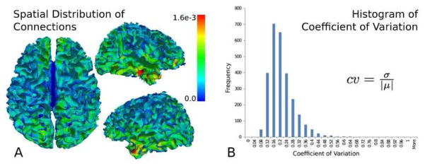
The population average nodal connection distribution, computed from the 2744 GM regions, mapped to the surface separating cortical grey and white matter of the template subject, is shown in Figure 6A. The population histogram (Figure 6B) of the coefficients of variation (the ratio of the standard deviation to the mean) of the nodes, shows all values to be below 0.7 with the majority below 0.5.

Figure 6.

The average nodal connection distribution (A) mapped to the grey/white matter surface. The nodal connections possess a rough bilateral symmetry, with areas of increased connections found in the temporal lobe. A histogram (B) of the nodes’ coefficient of variation (ratio of the standard deviation to the mean) shows values predominantly below 0.5, indicating the relative low variance of the nodal connection distribution in the population.

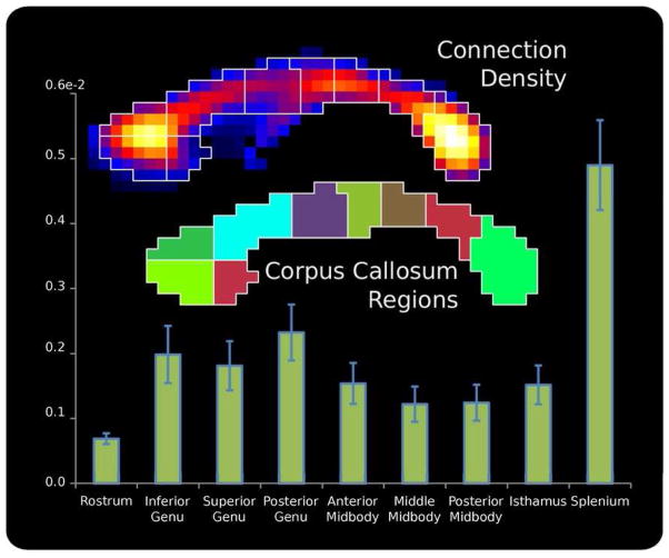
The corpus callosum (CC) is one of the few pieces of neuronal WM anatomy where the spatial distribution of the axons passing through have it has been studied, via histology. In order to facilitate comparisons between the proposed method and the invasive histological fiber counting methods, the spatial distribution of connections passing through the mid-sagital slice of the CC was examined. By summing the connection density images of each subject within each subregion of the CC the distribution of CC connections was determined. The population averaged connection density images of CC can be seen in Figure 7, as can the distribution of connections across 9 sub-regions of the CC.

Figure 7.

The spatial distribution of the connections through the mid-sagittal slice of the corpus callosum is shown. The distribution, with high concentrations in the splenium and genu, shows agreement with existing studies where fiber count was determined from histopathology (Highley, Esiri et al. 1999).

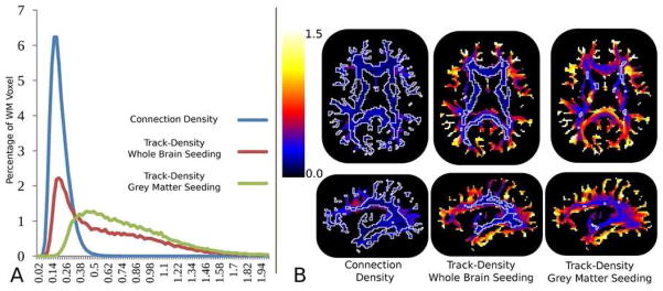
Additionally, we performed a comparison of the connection density images to an existing method, the track density images (TDI) generated using a probabilistic tracking algorithm seeded in all brain voxels (TDI-WholeBrain) as well as when seeded only in the GM (TDI-GM) nodal regions. TDI images were computed using a set of streamlines (N=750,000) determined via probabilistic tractography using the MRtrix (Brain Research Institute, Melbourne, Australia, http://www.brain.org.au/software/) software and the parameters specified in (Calamante, Tournier et al. 2010). The stopping threshold was decreased from 0.1 to 0.05, to provide a contrast similar to the images presented in (Calamante, Tournier et al. 2010). The coefficient of variation (CV), the ratio of the standard deviation to the mean, was computed for each WM voxel yielding a CV image for each of these three images, connection density, TDI-WholeBrain and TDI-GM. Representative slices of the CV images, as well as, a histogram of the CV values can be seen in Figure 8. A contour of CV=0.25 is overlaid on each image indicating areas that have a low population variance to mean ratio. Population average TDI-WholeBrain and Connection Density images can be seen in Figure 9. To provide a meaningful comparable contrast these images were normalized by their average values in the mid-sagital corpus callosum prior to performing the averaging.

Figure 8.

Coefficient of variation (CV) histograms, are shown in A, computed from the WM voxels of the connection density images, whole brain seeded and GM seeded track density images. Representative slices of the CV images are shown in B where the white line delineates the CV thresholded at 0.25 contour indicating areas of low population variance.

Figure 9.

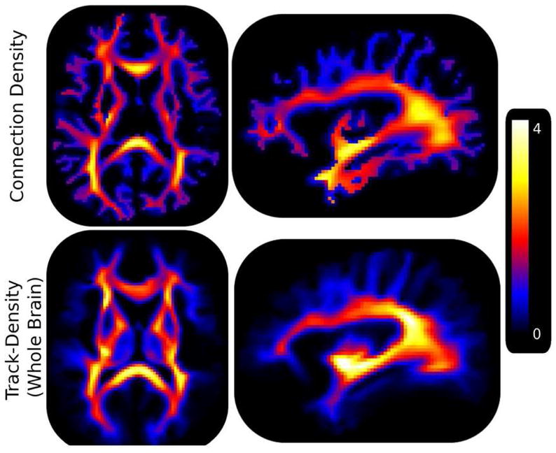
Population averaged track density images generated by seeding in the whole brain and connection density images are shown. Note that for visualization purposes each image was scaled by the number of connections passing through the mid sagittal corpus callosum prior to computing the average. These results indicate the higher contrast of the proposed method in cortical WM pathways, which are critical to the investigation of diseases that affect local connectivity, such as autism.

Discussion

As the use of structural connectivity to investigate population differences becomes more common place, the need for reliable, efficient and interpretable structural connectivity measures and methods will grow. The goal of this work is to present a methodology for investigating the structural connectivity of an individual that meets these standards. The method strives to produce results with a clear physiological underpinning, an interpretation based on the basic assumption equating particle trajectories with underlying anatomical pathways, as well as, the incorporation of physical constraints that reflect both the physiology and the information content of the imaging modality.

Our approach requires the explicit determination of the proportion of connections with an end in each node, a process based in the physiological expectations of connection symmetry as well as conservation of connections. It is important to note that DW-MRI, and thus the structural connectivity methods based upon it, have no means to distinguish between afferent and efferent axonal fiber bundles. Thus the expectations of symmetry are not based on ideas of functional connectivity and directionality of information transfer, but are simple physical constraints. Thus, symmetry of connection strength implies that the number of fibers, both afferent and efferent, connecting nodes A and B, should be the same as that found connecting B to A. Similarly, conservation of connections implies that the number of fibers terminating in node A should be equal to the number modeled exiting it.

For each subject, the method produces three features related to the structural connectivity: 1) The connectivity matrix, describing the proportion of connections between pairs of nodes, 2) The nodal connection distribution, describing the proportion of connections that terminate in each node and 3) the connection density image, which describes density of connections as they traverse through the WM. These features demonstrate a high degree of reproducibility of their respective components, the connectivity weights, GM nodes and WM voxels. This is evident by high (> 0.75) correlation coefficients, Figure 3A, and low (< 5%) percent error, Figure 3B. Additionally, for each of these three measures, the average difference, Figure 4, between the two time points of the same subject (Within) is roughly ¼ of the difference between different subjects (Between) at the same time point, indicating that these measures are specific to the individual. The combination of a repeatable and sensitivity within the proposed measures suggest that the proposed framework holds promise to elucidate population differences within group studies.

The population average structural connectivity matrix, downsampled to the anatomical nodes based on the Desikan atlas (Figure 5), displays the expected bilateral symmetry and is qualitatively similar to those found in the literature (Gong, He et al. 2009; Zalesky, Fornito et al. 2010). It is dominated by the diagonal elements, suggesting a high rate of short range self connections, when nodes are defined anatomically. At the higher resolution node parcellation, clear sub-circuits (Figure 5B) are visible, which are unavailable with the more typical anatomical nodes. For instance, the connections between the lateral occipital cortex (LatOcc) and the fusiform gyrus stem from a clearly defined sub network, highlighted in blue.

The ability to efficiently measure structural connectivity, with a high spatial resolution, offers a number of intriguing avenues of future research. Such high resolution connectivity profiles may prove useful in providing contrasts to cortical registration algorithms that currently utilize geometric features of the WM/GM boundary to drive the registration process. Similarly, they may improve cortical parcellations, providing better understanding of the functional/structural relationships between different regions and yielding more informative cortical atlases. This increase in spatial resolution does come at the expense of increasing the dimensionality of the connectivity matrix, causing statistical challenges when looking for group differences. However sophisticated dimensionality reduction techniques, such as manifold learning or sparse matrix decomposition, may be used to somewhat mitigate the loss of statistical power.

The nodal connection distribution (nCD) describes the proportion of connections that terminate in each node relative to the total number of connections in the connectivity network. Conceptually it is similar to the nodal weighted degree or nodal strength that has been used in other network analysis (Rubinov and Sporns 2010). As opposed to the nodal strength, which is computed from the connectivity matrix and is thus a feature of the network, the nCD is explicitly computed from the conditional probability matrix and plays a key role in imparting the framework as a whole with its physiological interpretation.

The population average nCD, seen in Figure 6A, displays a general bilateral symmetry that would be expected from a measure of anatomy. Variation in the nCD is visible, with bilateral increases in nCD in regions of the superior temporal lobe. While an explicit verification of the spatial pattern is not possible in this work, the population histogram (Figure 6B) of the coefficients of variation of the nodes indicates that it is fairly well preserved throughout the population. Additionally, this spatial contrast in connections lends credence to the idea that there exists topographical variability in the GM cytoarchitecture, such as the density of mini-columns (Casanova, El-Baz et al. 2010), which may affect the connectivity of various regions, suggesting that the nodal connection distribution may prove useful in localizing group differences or to serve as a feature used to improve GM parcellation schemes.

Finally, the connection density images provide a means to investigate and localize structural connectivity differences within WM volume, possibly enabling the identification of focal WM differences that may affect connections between a broad range of nodes. Figure 7 shows the connection densities of the mid-sagittal slice of the corpus callosum. We see that the majority of the connections pass through the splenium and the genu of the CC with a lower number in the mid-body. This spatial pattern has been seen in existing studies of CC which make use of histological fiber counting techniques to quantify the number of connections, as can be seen by comparing this result to Figure 5 of (Highley, Esiri et al. 1999).

When investigating the connection density in the whole of WM, we see that the proposed method has low CV values indicative of low population variance. The CV histograms of the connection density and TDI images, seen in Figure 8A, indicate that the connection density histogram is more concentrated in the lower ranges (CV < 0.5) indicating a tighter spread in the connection density across the population than in either of the TDI approaches. The spatial distribution of CV values, Figure 8B, show a concentration of low CV, less than 0.25 is indicated by the white contour, values in the central WM for the TDI image created using whole brain seeding and relatively few low CV values, when seeding from the GM exclusively. This is in contrast to the even spatial distribution of low CV values in the connection density image.

Images of the population averaged TDI-WholeBrain and connection density images, Figures 9, illustrate that the TDI images yield densities more concentrated in central WM pathways than in the cortical WM, whereas the contrast in the connection density image is much more balanced, emphasizing both the central pathways as well as the association or U fibers located in the cortical WM regions. Sensitivity to cortical WM is critically important to studies of development as well as some diseases such as autism where local connectivity is thought to be affected. It should be noted that the track density images presented here were generated using the tractography algorithm of MRtrix. Other tractography algorithms (Descoteaux, Deriche et al. 2009; Malcolm, Shenton et al. 2009) could be utilized and may give different results.

It is important to note that, without ground truth, it is difficult to quantitatively validate these or any method that attempts to quantify structural connectivity. The repeatability and sensitivity of the proposed measures (Figures 3 and 4) as well as their low population CV values (Figures 6-B and 7) are encouraging and indicate that testable hypothesis could be garnered from the spatial patterns of nodal connections (Figure 6A), as well as from the connection density images (Figures 7 and 9). A major strength of this work is the presentation of an integrated structural connectivity framework, where connection density images and connectivity matrices are products of a single methodology. Thus future corroborating evidence, validating aspects of the methodology, such as the spatial patterns evident in the nCD or the connection density images, would lend support to the framework as a whole, a particularly important fact considering the difficulty in validating whole brain structural connectivity matrices. The results of the validation, replication and application studies on the two datasets indicates the potential of the framework in elucidating group differences and in providing a unique means of identifying structurally homogenous GM regions.

By providing a representation of the physical connections between GM regions, structural connectivity networks provide a scaffold on which other functional (FMRI, MEG, etc) signals and information can be understood. The use of a single cohesive framework improves the ability of researchers to distinguish between different causes of connectivity deficits, such as focal changes in the underlying WM architecture (accessible by the connection density images) or by changes to the nodal connection patterns (obtained via an examination of the nodal connection distribution and connectivity networks). The ability of the framework to efficiently work with large networks, allows for higher spatial sensitivity, enabling finer node parcellations and a more detailed view of connectivity in the human brain.

Acronyms

WM

White Matter

GM

Grey Matter

CSF

Cerebrospinal Fluid

TDI

Track Density Imaging

nCD

Nodal Connection Distribution

DW-MRI

Diffusion Weighted Magnetic Resonance Imaging

HARDI

High Angular Resolution Diffusion Imaging

MC

Monte-Carlo fiber tracking

Mathematical Notations

S

State space of Markov process fiber tracking algorithm

N

Nodal Space for defining particle distributions

B

Linear operator mapping N to the boundary states of S

L

Linear operator mapping boundary states of S in N

T

Transition matrix describing the temporal evolution of the Markov process

C

The Conditional Probability Connectivity Matrix

M

The Structural Connectivity Matrix

References

- Aboitiz F, Scheibel AB, et al. Fiber composition of the human corpus callosum. Brain Res. 1992;598(1–2):143–153. doi: 10.1016/0006-8993(92)90178-c. [DOI] [PubMed] [Google Scholar]
- Anderson AW. Measurement of fiber orientation distributions using high angular resolution diffusion imaging. Magnetic Resonance in Medicine. 2005;54(5):1194–1206. doi: 10.1002/mrm.20667. [DOI] [PubMed] [Google Scholar]
- Balay S, Gropp WD, et al. Modern Software Tools in Scientific Computing. Birkh: 1997. Efficient Management of Parallelism in Object Oriented Numerical Software Libraries. [Google Scholar]
- Behrens TE, Woolrich MW, et al. Characterization and propagation of uncertainty in diffusion-weighted MR imaging. Magn Reson Med. 2003;50(5):1077–1088. doi: 10.1002/mrm.10609. [DOI] [PubMed] [Google Scholar]
- Bloy L, Ingalhalikar M, et al. White matter atlas generation using HARDI based automated parcellation. NeuroImage. 2011 doi: 10.1016/j.neuroimage.2011.08.053. [DOI] [PMC free article] [PubMed] [Google Scholar]
- Calamante F, Tournier JD, et al. Track-density imaging (TDI): super-resolution white matter imaging using whole-brain track-density mapping. NeuroImage. 2010;53(4):1233–1243. doi: 10.1016/j.neuroimage.2010.07.024. [DOI] [PubMed] [Google Scholar]
- Casanova MF, El-Baz A, et al. A topographic study of minicolumnar core width by lamina comparison between autistic subjects and controls: possible minicolumnar disruption due to an anatomical element in-common to multiple laminae. Brain Pathol. 2010;20(2):451–458. doi: 10.1111/j.1750-3639.2009.00319.x. [DOI] [PMC free article] [PubMed] [Google Scholar]
- Descoteaux M, Deriche R, et al. Deterministic and probabilistic tractography based on complex fibre orientation distributions. IEEE Trans Med Imaging. 2009;28(2):269–286. doi: 10.1109/TMI.2008.2004424. [DOI] [PubMed] [Google Scholar]
- Desikan RS, Segonne F, et al. An automated labeling system for subdividing the human cerebral cortex on MRI scans into gyral based regions of interest. NeuroImage. 2006;31(3):968–980. doi: 10.1016/j.neuroimage.2006.01.021. [DOI] [PubMed] [Google Scholar]
- Fischl B, Sereno MI, et al. Cortical surface-based analysis. II: Inflation, flattening, and a surface-based coordinate system. Neuroimage. 1999;9(2):195–207. doi: 10.1006/nimg.1998.0396. [DOI] [PubMed] [Google Scholar]
- Gong G, He Y, et al. Mapping anatomical connectivity patterns of human cerebral cortex using in vivo diffusion tensor imaging tractography. Cereb Cortex. 2009;19(3):524–536. doi: 10.1093/cercor/bhn102. [DOI] [PMC free article] [PubMed] [Google Scholar]
- Gong G, Rosa-Neto P, et al. Age- and gender-related differences in the cortical anatomical network. The Journal of neuroscience : the official journal of the Society for Neuroscience. 2009;29(50):15684–15693. doi: 10.1523/JNEUROSCI.2308-09.2009. [DOI] [PMC free article] [PubMed] [Google Scholar]
- Hagmann P, Cammoun L, et al. Mapping the structural core of human cerebral cortex. PLoS Biol. 2008;6(7):e159. doi: 10.1371/journal.pbio.0060159. [DOI] [PMC free article] [PubMed] [Google Scholar]
- Hagmann P, Kurant M, et al. Mapping human whole-brain structural networks with diffusion MRI. PloS one. 2007;2(7):e597. doi: 10.1371/journal.pone.0000597. [DOI] [PMC free article] [PubMed] [Google Scholar]
- Hagmann P, Sporns O, et al. White matter maturation reshapes structural connectivity in the late developing human brain. Proc Natl Acad Sci U S A. 2010;107(44):19067–19072. doi: 10.1073/pnas.1009073107. [DOI] [PMC free article] [PubMed] [Google Scholar]
- Heroux MA, Bartlett RA, et al. An overview of the Trilinos Project. ACM Transactions on Mathematical Software. 2005;31(3):397–423. [Google Scholar]
- Highley JR, Esiri MM, et al. The size and fibre composition of the corpus callosum with respect to gender and schizophrenia: a post-mortem study. Brain. 1999;122(Pt 1):99–110. doi: 10.1093/brain/122.1.99. [DOI] [PubMed] [Google Scholar]
- Iglesias JE, Thompson P, et al. Discretizing stochastic tractography: A fast implementation. Biomedical Imaging: From Nano to Macro, 2010 IEEE International Symposium on.2010. [Google Scholar]
- Iturria-Medina Y, Canales-Rodríguez EJ, et al. Characterizing brain anatomical connections using diffusion weighted MRI and graph theory. NeuroImage. 2007;36(3):645–660. doi: 10.1016/j.neuroimage.2007.02.012. [DOI] [PubMed] [Google Scholar]
- Iturria-Medina Y, Sotero RC, et al. Studying the human brain anatomical network via diffusion-weighted MRI and Graph Theory. Neuroimage. 2008;40(3):1064–1076. doi: 10.1016/j.neuroimage.2007.10.060. [DOI] [PubMed] [Google Scholar]
- Jezzard P, Barnett AS, et al. Characterization of and correction for eddy current artifacts in echo planar diffusion imaging. Magn Reson Med. 1998;39(5):801–812. doi: 10.1002/mrm.1910390518. [DOI] [PubMed] [Google Scholar]
- Konrad K, Eickhoff SB. Is the ADHD brain wired differently? A review on structural and functional connectivity in attention deficit hyperactivity disorder. Hum Brain Mapp. 2010;31(6):904–916. doi: 10.1002/hbm.21058. [DOI] [PMC free article] [PubMed] [Google Scholar]
- Malcolm JG, Shenton ME, et al. Neural tractography using an unscented Kalman filter. Inf Process Med Imaging. 2009;21:126–138. doi: 10.1007/978-3-642-02498-6_11. [DOI] [PMC free article] [PubMed] [Google Scholar]
- Robinson EC, Hammers A, et al. Identifying population differences in whole-brain structural networks: a machine learning approach. Neuroimage. 2010;50(3):910–919. doi: 10.1016/j.neuroimage.2010.01.019. [DOI] [PubMed] [Google Scholar]
- Rubinov M, Sporns O. Complex network measures of brain connectivity: uses and interpretations. Neuroimage. 2010;52(3):1059–1069. doi: 10.1016/j.neuroimage.2009.10.003. [DOI] [PubMed] [Google Scholar]
- Tournier JD, Calamante F, et al. Robust determination of the fibre orientation distribution in diffusion MRI: Non-negativity constrained super-resolved spherical deconvolution. NeuroImage. 2007;35(4):1459–1472. doi: 10.1016/j.neuroimage.2007.02.016. [DOI] [PubMed] [Google Scholar]
- Tristán-Vega A, Aja-Fernández S. DWI filtering using joint information for DTI and HARDI. Med Image Anal. 2010;14(2):205–218. doi: 10.1016/j.media.2009.11.001. [DOI] [PubMed] [Google Scholar]
- Yu Q, Sui J, et al. Altered Topological Properties of Functional Network Connectivity in Schizophrenia during Resting State: A Small-World Brain Network Study. PloS one. 2011;6(9):e25423. doi: 10.1371/journal.pone.0025423. [DOI] [PMC free article] [PubMed] [Google Scholar]
- Zalesky A, Fornito A, et al. Whole-brain anatomical networks: does the choice of nodes matter? NeuroImage. 2010;50(3):970–983. doi: 10.1016/j.neuroimage.2009.12.027. [DOI] [PubMed] [Google Scholar]