The Diffusion Tensor Imaging Toolbox

Abstract

During the past few years, the Journal of Neuroscience has published over 30 articles that describe investigations that used Diffusion Tensor Imaging (DTI) and related techniques as a primary observation method. This illustrates a growing interest in DTI within the basic and clinical neuroscience communities. This article summarizes DTI methodology in terms that can be immediately understood by the neuroscientist who has little previous exposure to DTI. It describes the fundamentals of water molecular diffusion coefficient measurement in brain tissue and illustrates how these fundamentals can be used to form vivid and useful depictions of white matter macroscopic and microscopic anatomy. It also describes current research applications and the technique’s attributes and limitations. It is hoped that this article will help the readers of this Journal to more effectively evaluate neuroscience studies that use DTI.

Introduction

In the first half of 2011, the Journal of Neuroscience published 14 articles describing studies that used Diffusion Tensor Imaging (DTI) or a related technique as a primarily observational methodology. Similar patterns are apparent in 2009 and 2010. This provides evidence of a growing interest in using DTI within the neuroscience research community. This interest results from DTI’s ability to make heretofore impossible measurements of the spatial organization of white matter (WM) at both macroscopic and microscopic spatial scales in living humans and living animals coupled with the growing enthusiasm for study of the brain ‘connectome’. This Toolbox article will introduce the key principles that underlie DTI methodology and will provide an overview of current DTI research applications together with attributes and current limitations of the technique. The small amount of available space makes the presentation somewhat superficial. It is impossible to fully explain all the nuances of DTI and to give credit to all who contributed to its present state of development in a short article. Readers wanting greater detail may wish to consult recently published books that are devoted entirely to DTI and related techniques (Mori, 2007; Johansen-Berg et al., 2009; Jones, 2010).

Measurement of water molecule diffusion with Magnetic Resonance Imaging

DTI is one of many imaging procedures that rely on magnetic resonance imaging (MRI) signal detection. In DTI, the measured MRI signal intensity is made to depend on the distance and direction the average water molecule in an image volume element (voxel) can move during a time period of approximately 100 msec. The measured signal intensity is processed to produce images in which intensity or color conveys some type of information about the water molecule motion. White matter shows prominent features in DTI and therefore DTI is often referred to as a WM imaging technique.

In the absence of a specific motive force, such as the oscillatory pressures that drive blood and cerebrospinal fluid (CSF) flows within the brain, water molecules move from position to position in a heat-driven random fashion that was initially described by Brown in 1828 (Brown, 1828). All students of the biological sciences become familiar with random ‘Brownian Motion’ at the time they first use of a microscope. Because there is no specific driving force, the direction in which any particular water molecule is moving at a particular point in time and its velocity are random unless the movement is constrained by barriers present within the tissue. Einstein quantitatively described the key features of Brownian Motion in one of the three famous publications he produced in 1905 (Einstein, 1905). An equivalent description was independently published by Smoluchowski in 1906 (Smoluchowski, 1906). Because of the intrinsic randomness of both direction and velocity, the Einstein-Smoluchowski description specifies only the average (mean square) distance that a molecule moves in a particular direction in a time period t as

$$<r^2>=2Dt$$ [1]

where D is known as the diffusion coefficient.

Measurement of water molecular diffusion by MRI is possible because hydrogen atomic nuclei are the primary source of the electromagnetic MRI signal. In brain tissue the detected MRI signal is primarily produced by the hydrogen nuclei within water molecules because of the high density of water relative to other hydrogen containing materials. In addition to density, other molecular factors can also be important in terms of producing MRI signal. For instance, it might be anticipated that in WM, the hydrogen atomic nuclei in the proteins and lipids that make up myelin membranes would be a significant signal source because myelin occupies a significant proportion of the WM volume. However this is not true. When the typical MRI signal acquisition procedures are employed, the hydrogen atoms must be able to freely rotate to be optimally detected. Myelin hydrogen atoms are so tightly constrained by the molecular structure that their signal is not detected with conventional MRI. Similarly water exists within the myelin membrane and can be detected by MRI. However the myelin-bound water has properties that make it hard to detect using DTI signal acquisition conditions. Thus even though DTI is usually described as a WM imaging technique and myelin is an important structural feature of WM, neither myelin nor myelin bound water signal detection is used in DTI.

Each hydrogen atom in each water molecule produces an oscillating electromagnetic signal. Each of these signals has three instantaneous properties: oscillation frequency, phase (i.e. the position in the oscillation cycle) and intensity. The MRI instrument measures the sum of the signals produced by all the hydrogen atoms that lie within each voxel of brain tissue. In order for the voxel signal to be readily detected, all the signals produced by the voxel must have coherent frequencies and phases. When the signals produced by a voxel become incoherent, the measured voxel signal is weakened due to destructive addition of signals having differing frequency and phase.

Signal detection depends on the existence of a rather strong static magnetic field, which is 3 T or larger for current day applications. A direct linear relationship exists between the signal frequency produced by each water molecule and the magnetic field strength at the point in space at which the molecule is located. DTI is similar to the most common types of MRI in using a ‘spin echo’ pulse sequence for signal detection (Figure 1). This pulse sequence initially creates the signals using an ‘excitation’ electromagnetic pulse delivered by a coil of wire located near the subject’s head. This pulse causes all the water molecules within the voxel to begin emitting signals having the same phase. The spin echo pulse sequence then has a waiting time, TE/2, during which this initial phase coherence can be lost. In DTI and related studies, it is specifically desirable to force loss of phase coherence during this TE/2 period. One of the ways of doing this is to activate a spatial magnetic field gradient. This gradient is referred to as a ‘diffusion sensitizing gradient’. Activating the gradient produces a situation in which the magnetic field is not identical at all points in the voxel and the water signals produced by the voxel have differing frequencies, develop different phases over a period of time, and destructively interfere with each other. Next the spin echo pulse sequence produces a second electromagnetic pulse at time TE/2. This pulse is referred to as a ‘refocussing pulse’. It has the effect of reversing the loss of coherence that developed in the prior TE/2 time period. It does this by adding a phase of one half the oscillation cycle to all signals. If the same gradient as was used during the first TE/2 period is again activated, and if there is little molecular movement, a strong coherent signal will be detected at a time TE/2 after the refocusing pulse. On the other hand, if there is significant molecular movement within the voxel between the first and second TE/2 times or during either TE/2 time, a weaker than expected signal will be detected because water molecules are located at different positions during the first and second TE/2 periods. It is possible to measure the amount of movement that occurs during the TE period by measuring signal level with and without activation of the diffusion sensitizing gradient. In DTI and related techniques the relevant motion that causes signal loss is Brownian diffusion motion.

Figure 1.

Key elements of the spin echo pulse sequence used for DTI. The timing of off/on (0/1) events for the three most important MRI scanner subsystems (Radiofrequency transmitter, Diffusion Sensitizing Gradient, and signal detection) is presented.

The principles underlying measurement of molecular diffusion in liquids was first published by Stejskal and Tanner in 1965 (Stejskal and Tanner, 1965). MRI was not known at the time. Stejskal and Tanner used conventional nuclear magnetic resonance spectroscopy detection to measure the diffusion coefficient in samples of liquid material. Their work was based on the (even then) widespread knowledge that spin echo signal intensity could be influenced by molecular diffusion when a static magnetic field gradient was present, as this was discussed in Hahn’s first paper describing the spin echo pulse sequence (Hahn, 1950). An expression for the signal change caused by diffusion can be derived for the pulse sequence shown in figure 1 using Stejskal-Tanner theory. In this pulse sequence, the magnetic field gradient is activated for a time period, δ, during each of the two TE/2 time periods with the separation between the leading edges of the two gradient pulses being Δ. The signal change produced by the diffusion motion in terms of the δ, Δ and the size of the diffusion sensitizing gradient, G, is given by Eqn [2]

$$\frac{S}{S_0}=e^{-{\gamma }^2{G}^2{\delta }^2\left(\mathrm{\Delta }-\frac{\delta }{3}\right)D}$$ [2]

S is the signal intensity that is measured when using the diffusion sensitizing gradient and S₀ is the signal intensity measured in its absence. The constant γ is a basic property of the hydrogen nucleus (the gyromagnetic ratio) that has a value of 2.675 × 10⁸ rad sec⁻¹ T⁻¹.

Le Bihan et al were the first to successfully apply these concepts to the human brain using MRI as a signal detection methodology (Le Bihan et al., 1986). They shortened the eqn [2] expression to

$$\frac{S}{S_0}=e^{-bD}$$ [3]

The term that expresses the effect of the diffusion sensitizing gradient is therefore now most often referred to today as the ‘b-factor’ or ‘b-value’. For the pulse sequence shown in Figure 1, the b-factor is given by

$$b={\gamma }^2{G}^2{\delta }^2\left(\mathrm{\Delta }-\frac{\delta }{3}\right)$$ [4]

In quantitative terms, eqns [2] or [3] show that measurement of the Einstein-Smoluchowski diffusion coefficient can be achieved by making a measurement of S₀ with b = 0 (by making G = 0), and then making a second measurement of S using some finite value of b (by setting the appropriate value of G). Thus S and S₀ are measured, b is known and D can be calculated from the measured data.

It is informative to consider the magnitude of the terms in eqns [3] and [4]. A present day human MRI scanner is capable of making a maximum gradient in each of the three principal directions of 45 mT m⁻¹. For such a scanner, when using a commercially available diffusion-weighted pulse sequence, the typical values of the diffusion sensitizing gradient pulse length and separation (δ and Δ) are (approximately) 35 and 40 msec. Hence Eqn [4] indicates the typical maximum b-factor that can be achieved by a present day human MRI scanner using a commercially available pulse sequence is approximately 1352 sec mm⁻². Normal mature brain tissue has a diffusion coefficient of about 800 μm² sec⁻¹. Eqn [3] indicates the signal change(S/S₀) when b = 1353 sec mm⁻² for normal brain tissue is therefore on the order of 0.45. If it is assumed that b equals 1353 sec mm⁻², that accurate measurement of (S/S₀) is feasible over the range 0.05 – 0.95, and that the effective diffusion time is Δ − δ/3, then Eqn [1] indicates that present day human brain DTI is sensitive to a root mean square water molecule displacement in a particular direction of 2 – 18 μm. From these calculations, it can be concluded that the so-described diffusion measurement is sensitive to water movement on a ‘microscopic scale’. It is important to understand that this conclusion has nothing to do with the spatial resolution used for imaging, which for human brain DTI is typically 2 – 3 mm. The description pertains to the measurement of the average Brownian diffusion behavior of the water molecules in whatever the ‘volume of interest’ happens to be, which in the context of MRI signal detection is usually the imaging voxel. Thus, while the DTI technique measures microscopic motion, it does so by averaging the diffusion properties over a great many cells and axons.

The b-factor limit of 1353 sec mm⁻² given in the preceding paragraph is not a particularly hard limit. Larger b-factors are achievable if δ and Δ are increased when commercially available diffusion weighting pulse sequences are used or by use of custom pulse sequence designs (which are usually not commercially available.) Larger b-factors are desirable because they provide increased sensitivity to the diffusion effect. Moreover increased b-factors make the measurement sensitive to diffusion on a smaller spatial scale. For instance if a b-factor of 3000 sec mm⁻² is used in the calculations given in the preceding paragraph with the same δ and Δ values, the measure becomes sensitive to a root mean square water molecule displacement in a particular direction of 2 – 12 μm. The advantages of increased b-factor are counterbalanced by two negative features. First, larger b-factors produce smaller diffusion-weighted signal and the intrinsic noise associated with MRI signal detection can become an important accuracy limiting factor.

Second, if the b-factor is increased by increasing the δ and Δ values additional signal loss unrelated to diffusion will be present. This additional signal loss is the result of transverse (T2) relaxation that is occurring simultaneously with the diffusion sensitization. Description of this relaxation process is beyond the scope of this article, but the magnitude of signal change it produces is similar to that produced by diffusion. The counterbalancing goals of having strong diffusion weighting (i.e. large b-factor) and enough signal to accurately measure has lead to widespread use of ‘intermediate’ b-factors of approximately 1000 sec mm⁻² in human brain DTI studies.

MRI is intrinsically an imaging technique. Accordingly, the diffusion coefficient measurement is actually made over a 3-dimensional grid of voxels that cover almost the entire brain and the results are (usually) presented as quantitative images. Figure 2 provides an illustration of a diffusion coefficient image in which the gray scale image intensity reports the numerical value of D at each point in the imaged plane. The gray scale level shows that most of brain water has a diffusion coefficient of approximately 800 μm² sec⁻¹. The larger image intensity that is present in the CSF space is a consequence of the fact that water in the CSF space can diffuse more freely than can brain tissue water because of the absence of cells and barriers to diffusion motion.

Figure 2.

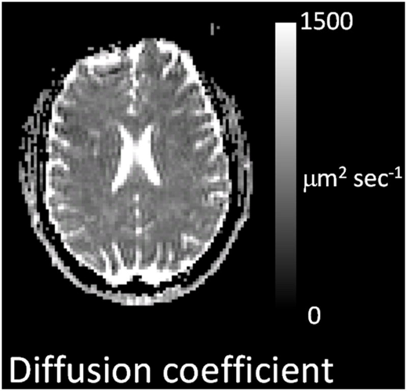
Quantitative image of diffusion coefficient from a normal human subject. The grayscale to right of the image indicates that image intensity represents the quantitative value of the diffusion coefficient (also referred to as diffusivity) of the brain tissue. Specifically this is an image of Mean Diffusivity defined by Eqn [12] (see text).

The current day spatial resolution limit for whole brain human DTI is approximately 2 mm. This statement assumes that 1) whole brain coverage is desired, 2) commercially available pulse sequences (that have been cleared by the relevant regulatory authority) are used, 3) a b-factor of approximately 1000 sec mm⁻² is used, 4) a reasonable degree of directional sampling (described in the next section) is used and 5) the total acquisition time is less than 15 min. These requirements are typical in present day neuroscience DTI studies of humans. Relaxing one or more of these requirements can be helpful if is desired to have improved resolution. In this context, there are a great many details and complex issues related to the design of diffusion weighted pulse sequences and to MRI scanner hardware performance that can not be covered in a short article such as this. DTI studies of rodents or fixed tissue samples can be performed using significantly better spatial resolution because of the smaller physical size of the necessary equipment, which facilitates use of substantially stronger gradients and provides increased signal-to-noise ratio per unit volume. Moreover studies of rodents (which usually involve anesthesia) or fixed tissue samples typically have less stringent acquisition time requirements in comparison with studies of awake humans. Longer acquisition times allow averaging of repeated measurements to enhance image quality.

Directionally specific measurements

The foregoing discussion ignores the possibility that there may be directional constraints on the microscopic diffusion movement of water molecules. DTI specifically takes this possibility into account by measuring how the diffusion coefficient depends on direction in every volume element of the image space. This section introduces concepts that help to explain why DTI is sensitive to the microscopic directional constraints that are present in brain WM and how the directionally sensitive measurements are made.

While in principle, any kind of microscopic structure may be important in imposing directional constraints on the diffusion movement of water molecules, the most significant microscopic feature seems to be organized arrays of myelinated axons in WM. In mature brain, it is only WM that produces a readily measured directional effect. As a result, DTI has become known as a ‘white matter imaging’ technique. This oversimplification results from the fact that, although microscopic diffusion barriers are present in gray matter (GM) and, in fact, create a measurably smaller GM diffusion coefficient compared to the CSF diffusion coefficient, the GM barriers do not have the same easily measured directional impact as the presence of arrays of myelinated axons seems to have in WM. Although WM is the current focus of DTI-related efforts, GM is also important. There have been successful efforts to detect preferential directional diffusion related to neuronal migration in premature GM (Neil et al., 1998) and direction effects in mature GM diffusion have considerable clinical and neurobiological importance although these may be difficult to accurately measure.

A concept diagram illustrating the principles of WM DTI is presented in figure 3. The colored lines in this figure show simulations of random movement over the time of a small group of water molecules that started out at the same point in space. Water molecules that were initially very close to each other move away in a random fashion. In CSF the average distance moved per unit time is larger than in GM or WM due to the absence of internal barriers. In WM the most prominent internal barriers are usually assumed to be the axonal membranes, which are myelinated in mature brain. These membranes are depicted as solid black lines in the figure. Further development of the DTI concept assumes that the WM ‘imaging voxel’ contains an array of densely packed axons that are parallel to each other. From the colored diffusion trajectories, it can be appreciated that the diffusion rate perpendicular to the axon array is smaller than it is in the direction parallel to the array. Because of this, diffusion in this array of axonal structures is said to be directionally anisotropic. Diffusion in the CSF and GM structures is directionally isotropic. Thus if the diffusion sensitizing gradient is oriented perpendicular to the axon array, more signal will be detected with diffusion weighted MRI than would be the case when the diffusion sensitizing gradient is oriented parallel to the axon array. Furthermore when the diffusion sensitizing gradient is oriented parallel to the axon array the diffusion signal attenuation in WM should be approximately the same as in GM and somewhat less than is observed in CSF. Such features can be appreciated in the diffusion weighted images from human brain shown in figure 4. Midline callosal signal attenuation is more pronounced when the diffusion sensitizing gradient is oriented parallel to the midline callosal fibers (i.e. in the left-right direction) compared to when it is oriented in the perpendicular direction (i.e. anterior-posterior direction). Figure 4 also shows similar gradient direction dependent signal intensity differences in WM fiber structures that are primarily oriented in the anterior-posterior direction and in fiber structures oriented in the superior-inferior direction in this particular brain section. Furthermore GM signal does not change when the diffusion sensitizing gradient direction is changed because of the absence of directional diffusion restrictions in GM.

Figure 3.

DTI concept diagram. The middle panel illustrates water molecule diffusion trajectories in CSF, white matter and gray matter. The top and bottom panel illustrate the effect of gradient sensitizing direction on MRI signal intensity from these tissue regions. See text for further details.

Figure 4.

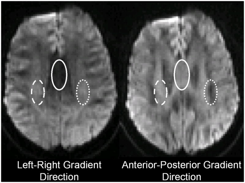
Diffusion weighted images from a normal human subject obtained with two different diffusion sensitizing gradient directions. These are 4 mm thick sections acquired with diffusion-weighted spin echo echo planar imaging using a b-vector magnitude of 1000 sec mm⁻² with the b-vector directed along the left/right axis (left panel) and the anterior/posterior axis (right panel). Ovals identify differing signal characteristics in three major white matter pathways (left-right oriented corpus callosum spenium (solid oval), anterior-posterior oriented temporofrontal pathway (dotted oval) and rising/descending pyramidal tracts (dashed oval)).

Figure 3 assumes the WM diffusion coefficient parallel to the axonal array is equal to the GM diffusion coefficient measured in any direction. This assumption was used to simplify the comparisons made in the illustration. It may not be generally true for all WM structures. In fact WM often shows a diffusion coefficient measured in the direction parallel to the axonal array that is much greater than the typically measured (in any direction) GM value (~ 800 μm² sec⁻¹). The purpose of figure 3 is not so much to report absolute values of the normal GM and WM diffusion coefficients, but to illustrate why diffusion coefficients measured in WM are directionally anisotropic.

Readers should be aware that the concepts presented in figure 3 are also superficial in the sense that there is not wide agreement that the myelinated axonal membrane is the actual diffusion barrier. Here the primary contradictory evidence is that immature unmyelinated axon arrays show measurable anisotropic diffusion characteristics (see for example (Baratti et al., 1999) (Larvaron et al., 2007; Gao et al., 2009)). However on the other hand, sequential measurements done during brain development show that the diffusion coefficient measured in the direction perpendicular to axon array decreases substantially during myelination in rodents and humans(Larvaron et al., 2007; Gao et al., 2009).

The DTI measurement was initially described by Basser et al (Basser et al., 1994) in 1994. This was the first effort to systematically measure the directional characteristics of diffusion with MRI. This followed about a decade of world-wide effort to substantiate clinical and experimental use of diffusion weighted imaging in which directional constraints on brain water diffusion were not specifically taken into account. During this period the anisotropic nature of water diffusion in WM was known to exist (see for example (Moseley et al., 1990a)), but it was viewed as more of a problem than an opportunity. Efforts were focused on developing diffusion weighted image acquisition schemes and image analysis techniques that suppressed or averaged out the anisotropic nature of WM diffusion. The most well established of these rotationally-independent measures was the apparent diffusion coefficient (ADC), which was defined by Moseley as the average of the diffusion coefficients measured in the MRI scanner’s x, y and z directions.

DTI takes advantage of the fact that virtually all MRI scanners have three hardware systems that are designed to create linear magnetic field gradients in the three principal directions of the scanner’s coordinate system. The ‘x-gradient’ system may be used to measure the diffusion coefficient along the ‘x-direction’, which is usually assumed to be the left-right axis of the scanner. The y- and z-gradients systems can be used to make the corresponding measurements along the y and z directions, which are usually assumed to be the scanner’s floor-ceiling and center axes. The diffusion coefficient along any arbitrary direction may be measured by using combinations of the three gradient systems to form a magnetic field gradient having an arbitrary orientation in space

$$\mathit{G}=G_x\left[\begin{array}{c}\mathbf{1}\\ \mathbf{0}\\ \mathbf{0}\end{array}\right]+G_y\left[\begin{array}{c}\mathbf{0}\\ \mathbf{1}\\ \mathbf{0}\end{array}\right]+G_z\left[\begin{array}{c}\mathbf{0}\\ \mathbf{0}\\ \mathbf{1}\end{array}\right]$$ [5]

In eqn [5] and the remainder of the article, boldface typescript is used to represent vector or tensor quantities. In eqn [5], G_x, G_y and G_z represent the gradient created by the three gradient hardware systems. The directional properties of the gradient are expressed in eqn [5] by multiplying vectors of unit length ([1, 0, 0], [0, 1, 0], [0, 0, 1]) by the gradient amplitudes produced by each of the three hardware systems and summing. From eqn [5] it can be seen that it is possible to create a gradient in any arbitrary spatial direction by choosing the appropriate values of G_x, G_y and G_z, between 0 and the maximum that the three gradient hardware systems can produce. This makes it possible to measure diffusion in any arbitrary spatial direction as will be shown below.

Substitution of eqn [4] into eqn [5] demonstrates that for DTI studies, the b-factor is a vector quantity.

$$\left[\begin{array}{c}{\mathit{b}}_{\mathit{x}}\\ {\mathit{b}}_{\mathit{y}}\\ {\mathit{b}}_{\mathit{z}}\end{array}\right]={\gamma }^2{\delta }^2\left(\mathrm{\Delta }-\frac{\delta }{3}\right)\left(G_x^2\left[\begin{array}{c}\mathbf{1}\\ \mathbf{0}\\ \mathbf{0}\end{array}\right]+G_y^2\left[\begin{array}{c}\mathbf{0}\\ \mathbf{1}\\ \mathbf{0}\end{array}\right]+G_z^2\left[\begin{array}{c}\mathbf{0}\\ \mathbf{0}\\ \mathbf{1}\end{array}\right]\right)$$ [6]

The corresponding analog of the Einstein-Smoluchowski diffusion coefficient used in DTI studies is the diffusion tensor, D,

$$\mathit{D}=\left[\begin{array}{ccc}{D}_{xx}& D_{xy}& D_{xz}\\ D_{yx}& D_{yy}& D_{yz}\\ D_{zx}& D_{zy}& D_{zz}\end{array}\right]$$ [7]

D is usually assumed to be a diagonally symmetric matrix and therefore only 6 of the 9 elements are unique.

$$\mathit{D}=\left[\begin{array}{ccc}{D}_{xx}& D_{xy}& D_{xz}\\ D_{xy}& D_{yy}& D_{yz}\\ D_{xz}& D_{yz}& D_{zz}\end{array}\right]$$ [8]

This is a mathematical expression of the assumption that the diffusion is symmetric in any particular direction. In other words forward diffusion along a particular direction has equal probability as backward diffusion along the same direction. The diffusion tensor serves as a convenient mathematical tool to express the directional dependence of Einstein-Smoluchowski diffusion. If the values of the 6 tensor terms are known, it is possible to calculate the value of the diffusion coefficient in any arbitrary direction in space. For instance if it was desired to know the value of the diffusion coefficient along a direction r = [r_x, r_y, r_z], one would perform the calculation shown in equation [9] using the rules of matrix multiplication. (Readers who are unfamiliar mathematical operations on vectors and matrices are urged to consult a text book or website on linear algebra.)

$$D_r=[r_x{r}_y{r}_z]\left[\begin{array}{ccc}{D}_{xx}& D_{xy}& D_{xz}\\ D_{xy}& D_{yy}& D_{yz}\\ D_{xz}& D_{yz}& D_{zz}\end{array}\right]\left[\begin{array}{c}{r}_x\\ r_y\\ r_z\end{array}\right]$$ [9]

In eqn [9], the vector r is assumed to have unit length but to point in the direction of interest.

The corresponding DTI ‘signal equation’ (ie the DTI analog of eqn [3]) is

$$\frac{S}{S_0}=e^{-Tr(\mathit{bD})}$$ [10a]

In eqn [10], D is the diffusion tensor, b is a matrix defined in eqn [11] and ‘Tr’ designates the mathematical ‘trace’ operation (i.e., to sum the diagonal elements of the matrix being operated on).

$$\mathit{b}={\gamma }^2{\delta }^2\left(\mathrm{\Delta }-\frac{\delta }{3}\right)\left[\begin{array}{ccc}{G}_x{G}_x& G_x{G}_y& G_x{G}_z\\ G_y{G}_x& G_y{G}_y& G_y{G}_z\\ G_z{G}_x& G_z{G}_y& G_z{G}_z\end{array}\right]$$ [11]

Eqn [10] indicates how the measured signal intensity will depend on the orientation and the magnitude of the b-matrix (which is defined by choice of gradient strengths G_x, G_y, G_z) and the orientation of the diffusion tensor. Therefore the general strategy of a DTI measurement is to perform a series of image acquisitions using a unique b-matrix for each acquisition. The signal intensities measured in this series of images will depend on the values of the diffusion tensor elements. If enough image acquisitions are performed using unique appropriately chosen b-matrices, it is possible to determine the values of the diffusion tensor elements.

At this point it is important to emphasize that the expressions given in eqns [5] – [10] represent an ‘ideal’ situation that only approximates the true situation encountered in a real measurement of diffusion in the brain. These expressions are presented to help ground reader in past development work and also to provide a basis on which a real measurement can be understood. Two major deviations from these ideals may exist. 1) The actual values of the b-matrix elements depend on the detailed structure of the entire pulse sequence. Gradient pulses are used as part of the imaging process and these imaging gradient pulses may alter the directional diffusion sensitivity. Furthermore even if imaging gradient pulses are ignored, eqn [6] is absolutely correct only when the diffusion sensitizing gradient pulses are rectangular as shown in figure 1. Alteration of the shape of gradient pulses provides some advantages, such as increased b-factor or reduced TE, and pulse sequences that are used in real studies do not necessarily use such rectangular gradient pulses. In general, it is possible to calculate the values of the b-matrix elements if the exact structure of the pulse sequence is known (Mattiello et al., 1997). However further empirical calibration is sometimes also necessary because the three gradient systems may not perform ideally. 2) Einstein-Smoluchowski diffusion may not model the true diffusion characteristics in all WM areas of the brain. For instance brain regions lying at the interface between WM and CSF may be better modeled using a mixture of two diffusion tensors, one that describes the isotropic nature of CSF diffusion and the other that describes the anisotropic nature of WM diffusion. Similarly regions in which there is within-voxel curvature of the WM fiber array or in which different WM fiber bundles intersect each other may require more complex expressions than a single diffusion tensor to characterize them.

Making directionally-specific diffusion coefficient measurements in an anatomically complex organ like the brain requires somewhat a more complicated measurement strategy than had been used in preceding DWI studies. The scanner makes gradients, and therefore measures diffusion coefficients, in its own fixed reference frame but the axonal structures of interest at any spatial location in the brain will not necessarily be aligned with the scanner coordinate system. This mandates measurement of the diffusion using an array of directionally sensitized submeasurements. This is done by sampling the diffusion characteristics in a multiplicity of directions (i.e. by performing a series of measurements with varying b-matrices and then assembling the acquired data in a logical way). Usually the directional sampling is uniform over 3-dimensional space. There are 7 unknown parameters (S₀ and the six unique elements of the diffusion tensor). A minimum of 6 unique directionally-sensitized intensity measurements and at least one non-diffusion-sensitized measurement are therefore necessary to estimate all unknown parameters. Accordingly in the most simplistic DTI measurement, one imaging study is performed with b = 0 (no diffusion sensitizing gradients) and at least 6 additional image acquisitions are performed with the b-matrix having finite magnitude and variable orientation. The collection of additional data (image acquisition with more than one b = 0, more than 6 directions of sampling, and use of more than one high b factor) can considerably improve the estimate of the diffusion tensor elements. However each of the additional image acquisitions takes time and thereby has an associated cost and potential for artifact introduction and there tends to a practical limit. Typical current day DTI studies used in routine human neuroscience studies sample 20 – 64 b-matrix directions using two b-factor amplitudes, one of which is approximately zero, with the other of has an amplitude of approximately 1000 sec mm⁻². Advanced studies have used as many more unique directionally sensitized acquisitions. Such measurements are frequently referred to as High Angular Resolution Diffusion Imaging (HARDI) or (HARD), a term that appears to have first been coined by Frank (Frank, 2001). In addition to high angular resolution directional sampling, the initial HARDI studies used b-factors much larger than 1000 sec mm⁻², because doing so is reported to provide an enhanced ability to identify the true direction in which an array of whiter matter fibers are aligned. However in recent years, some authors who use b-factors in the 1000 – 1500 sec mm⁻² range have been referring to their studies as HARDI studies, just because they use a high degree of directional sampling. Some more sophisticated studies also use multiple b-factor weighting in addition to multiple directionally sensitized acquisitions. These go by various names. One of these is ‘Q-Ball’ or ‘Q-space’ imaging (Tuch, 2004) because the Fourier Transform of the signal versus b-factor is known as Q-space. Another advanced procedure that uses a combination of multiple b-factor weightings and many directionally sensitized acquisitions is known as Diffusion Spectrum Imaging (DSI) (Wedeen et al., 2005). Here it is important to state that the present author takes the point of view that these various sampling methodologies and their associated postprocessing techniques are subparts of a ‘general DTI’ methodology while other investigators sometimes argue that DTI should be used only as a term for the methodology originally proposed by Basser (Basser et al., 1994) (i.e. 7 acquisitions and data reduction involving 3 × 3 tensor analysis).

In the originally proposed DTI approach the diffusion tensor’s six unique elements are determined by solving a system of signal equations using the measured signal values made with the directionally-specific b-factors. For studies involving WM it is usually then desired to determine the directional orientation of the (assumed) axonal fiber array for each voxel in the imaged space. To do so, it is assumed that the direction that has the largest diffusion coefficient is parallel to the fiber structure. Determining this ‘principal’ direction that shows the largest diffusion coefficient from the measured diffusion tensor can be performed in a variety of ways. The most commonly used computational technique decomposes the diffusion tensor (measured at each voxel) into a set of three characteristic perpendicular vectors, one of which is aligned in the direction that has the largest diffusion coefficient. In mathematics this is known as eigenvector decomposition. However it is sometimes significant to know that use of the eigenvector decomposition formalism is possible in this instance only because of the (assumed) symmetry of the diffusion tensor. Because the eigenvector decomposition approach is used so frequently, the direction of the WM fiber array alignment within each voxel is often referred to as the ‘principal eigenvector’. Two other ‘eigenvectors’ that define directions perpendicular to the principal eigenvector are also derived. Each of the eigenvectors has a corresponding ‘eigenvalue’ that are also produced by the decomposition procedure. The eigenvalues are just the directionally specific Einstein-Smoluchowski diffusion coefficient in the direction specified by their corresponding eigenvector. The eigenvalues are usually given the symbol λ and are usually referred to as λ₁, λ₂, λ₃, with λ₁ being the principal eigenvalue which is larger than λ₂ and λ₃. For WM it is sometimes assumed that λ₂ equals λ₃ and the diffusion is said to display ‘axial symmetry’. Images that convey the value of the diffusion coefficients (equivalent to the eigenvalues) are sometimes presented in DTI studies. These may be images of λ₁, λ₂ and λ₃ or images of Mean Diffusivity (MD)

$$MD=\frac{1}{3}({\lambda }_1+{\lambda }_2+{\lambda }_3)$$ [12]

the Axial Diffusivity (AD)

$$AD={\lambda }_1$$ [13]

or the Radial Diffusivity (RD)

$$RD=\frac{1}{2}({\lambda }_2+{\lambda }_3)$$ [14]

Examples are shown in Figure 5. Of these, the RD is believed to be most useful for evaluation of a diseases involving myelin, because the radial diffusivity is believed to be primarily dependent on myelin barriers. In some cases Tr(D) is used instead of MD because the trace of the diffusion tensor is equivalent to the sum of the eigenvalues,

Figure 5.

DTI results images (FA, CM, AD, RD, MD) from a normal human subject. A T1-weighted image (T1wMRI) that depicts the traditional MRI view of brain anatomy has been aligned and resliced to match the DTI images. These images illustrate that DTI provides directional information about white matter fiber array orientation that is not present in traditional T1-weighted MRI and that DTI provides quantitative images of water diffusivity parallel to an perpendicular to the fiber array orientation. The color system used for the CM is displayed to the lower right of the CM. The CM allows the reader to immediately visualize the directional orientation of the primary eigenvector in the left-right, anterior-posterior, superior-inferior co-ordinate system.

In addition to λ₁, λ₂, λ₃, MD and RD, a simple summary image can be formed of the ‘Fractional Anisotropy’ (FA) (Basser and Pierpaoli, 1996).

$$FA=\sqrt{\frac{{({\lambda }_1-{\lambda }_2)}^2+{({\lambda }_1-{\lambda }_3)}^2+{({\lambda }_2-{\lambda }_3)}^2}{2({\lambda }_1^2+{\lambda }_2^2+{\lambda }_3^2)}}$$ [15]

FA provides an easy to calculate index that conveys how much larger λ₁ is compared with λ₂ and λ₃. The FA index approaches 1 when the principal eigenvalue is much larger than the other two eigenvalues. Brain regions showing high FA are thereby assumed to contain well organized parallel axon arrays. The FA index approaches zero when the three eigenvalues are equal and regions showing this FA characteristic are assumed to be gray matter or to be some other tissue type that does not have a great deal of internal directional organization such as CSF. It is also possible to form a colorized image that helps to convey the direction of the principal eigenvector (Pajevic and Pierpaoli, 2000). Figure 6 provides an example of a DTI ‘ColorMap (CM)’ in which Red-Blue-Green color system shows the principal eigenvector’s direction. Usually the intensity of color in such images is also weighted by FA to reduce the influence of non-WM tissues.

Figure 6.

Three-dimensional volume renderings of DTI CM. Left lateral, frontal and cranial views are provided. These images are presented to illustrate that DTI results are 3-dimensional image volumes. The color system is the same as that used in figure 5

The example images shown in the figures provide only one 2 mm thick image slice for clarity of presentation. In fact, the typical DTI study collects image data as multiple parallel slices from which entire brain volumes can be constructed. This is illustrated in Figure 6, which shows 3-dimensional renderings of DTI CMs.

The majority of current day DTI studies limit analysis and results evaluation to the diffusivity measures (MD, AD, RD, FA) and CMs. The diffusivity and FA images have convenient properties that make them useful for analyses involving groups of individuals. The values of diffusivity parameters are ‘rotationally invariant’, meaning that the results should not have a dependence on exactly which set of diffusion sensitizing gradients were used or how a particular individual’s head was positioned in the scanner. This is generally not true for CMs unless the color direction system has been specifically aligned to the anatomy. While reformatting the data to form rotationally-invariant diffusivity images provides the opportunity for further evaluation using the same computational brain mapping techniques that are used for analysis of multi-subject morophometric or functional neuroimaging data, some caution must be exercised (Jones and Cercignani, 2011).

Advanced DTI measurements and analyses

DTI technology is presently in active evolution. New, better and different approaches to DTI acquisition and data analysis appear each year. Several general themes of this evolution process are described in the following paragraphs of this section.

The eigenvector information may be used to perform a tractography analysis (Basser et al., 2000). The product of the tractography analysis is an image of a 3-dimensional model that uses curved 3-dimensional lines or tubes to represent the 3-dimensional directional organization of WM over the entire brain or to represent specific WM tracts. In principle tractography provides a means for study of the anatomic WM connections between specific GM areas in cortex or deep nuclei. A simple example is provided in figure 7. Generally speaking, two primary forms of tractography (deterministic and probabilistic tractography) now exist (for a review of tractography approaches see (Jones, 2008)).

Figure 7.

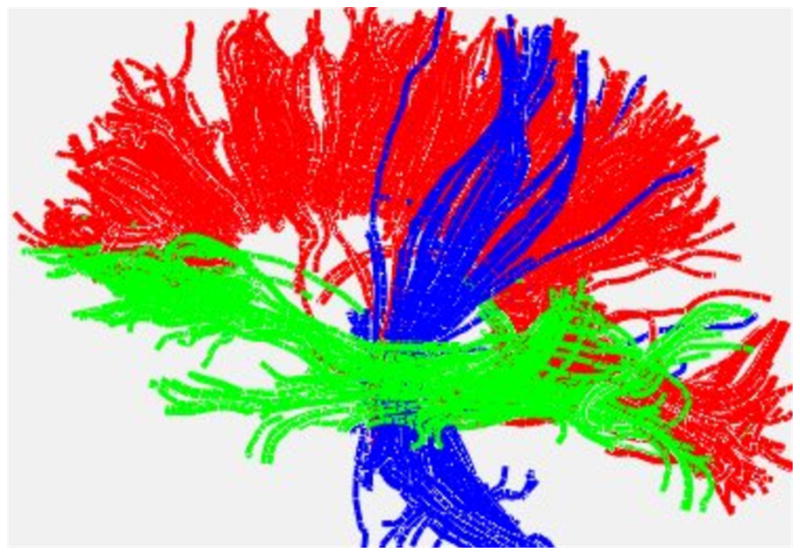
Fiber tractography of major white matter systems in a normal human subject: A left lateral view showing white matter structures passing through the corpus callosum (red), rising-descending pyramidal pathways (blue) and fronto-temporo-occipital pathways (green) are presented. Tractography was performed with DTIStudio/MRIStudio (www.mristudio.org).

The most common form of deterministic tractography is uses a ‘streamline’ approach to follow the principal eigenvector direction from voxel to voxel over long distances. In this approach the principal eigenvector direction (of each voxel) is used to create a 3-dimensional field of vectors. Computational techniques similar to those developed for aerodynamic simulations and weather forecasting can then be used to construct a set of streamlines that follow the vector field. The streamlines are typically edited by the user to show only the streamlines that connect regions of interest. Tractography software implementations usually allow the user to specify anatomic regions-of-interest that define where the streamlines begin or end or define some midpoint along lines. The user is frequently also permitted to specify a minimal FA level for streamline termination. Streamlines that encounter a voxel having FA below the specified minimum level are terminated. Similarly, the user is frequently also able to specify a maximum turn angle. Streamline that are bent through an angle that is greater than the specified maximum angle are terminated or allowed to follow a weaker vector field that does not turn so abruptly. User specified minimal FA values and maximal turn angles help to filter out streamlines that are anatomically unrealistic due to inaccuracy in the diffusion tensor measures, which is often related to noise present in the raw diffusion-weighted images.

Probabilistic tractography is an enhancement of deterministic methodology which takes into account that there is uncertainty (i.e experimental error) associated with the determination of the principal eigenvector’s orientation at each point in the imaged space (Behrens et al., 2003). Typically a ‘cone of uncertainty’ which specifies the distribution of probable orientations of the principal eigenvector for each voxel is estimated. Deterministic tractography is then performed a large number of times with the principal eigenvector orientation being chosen at random within constraints determined at random from the cones of uncertainty. The results from the large number of streamline studies are then assembled to produce statistical estimates of the anatomic connections between a seed point and a termination point. Such probabilistic methods provide a quantitative statistical inference of the anatomic connections that exist between seed point and a termination points.

Once a tract has been identified (by either general method), certain characteristics of the tract, such as the FA or the diffusivities within the tract, can be measured. Results of these measurements can then be assembled across the study population to form ‘tract-based spatial statistics’ (TBSS) (Smith et al., 2006) which are sometimes presented in image format.

Another advanced analytic procedure involves calculation of detailed geometric models of the directional dependence diffusion for each voxel. The tensor modeling approach that has been described above amounts to a relatively ‘low resolution’ approach for encapsulating the magnitude and the directional dependencies of water diffusion. Advanced techniques use a variety of analytic and modeling approaches to derive higher angular resolution geometric models and to thereby to produce a more accurate estimation of the true orientational distribution function (ODF). Such methods generally require the collection of HARDI data. These efforts grew from earlier procedures that presented the diffusion coefficient information as prolate or oblate ellipsoids or spheres that conveyed the orientation of the diffusion tensor in 3-dimensional space (Figure 8). As HARDI acquisitions became more feasible, it became possible to create more geometrically sophisticated spatial models (Tuch, 2004; Anderson, 2005; Wedeen et al., 2005) of the voxel diffusion information. Many authors argue that such complex spatial modeling is helpful in terms of identifying diffusion constraints that exist within the voxel (i.e. at a spatial scale that is well below the image acquisition resolution). The underlying rationale has been that one can use the highly detailed angular diffusion information to interpolate the internal structure of the WM within a voxel. This is particularly attractive in terms of resolving fine scale features, such as fiber bundles that intersect each other within a voxel or to more accurately follow curvature, convergence and divergence of fiber bundles within a voxel (Alexander, 2005; Wedeen et al., 2005). Perhaps more importantly, such highly refined views of sub-voxel WM structure might provide clues about cellular pathophysiological processes that occur in WM disease or to clarify how other subject characteristics of interest such as genetic profile or intellectual aptitude might relate to WM microscopic structure.

Figure 8.

The left panel is a depiction of the diffusion ellipsoid derived from the diffusion tensors measured in each image voxel in a single 2 mm axial slice. Each ellipsoid is represented as a color coded 3-dimensional object. Color coding reflects the direction of the principal eigenvalue using the color system defined in figure 5. The right panel shows a magnified view of the region around the genu of the corpus callosum.

Attributes

DTI encapsulates many significant innovations and attributes that have led to its profound growth over past few years. Several of the more important of these are described in this section.

While many current DTI studies are targeted at understanding the large and small scale structure of WM, this evolved from earlier work on quantitative imaging of the water diffusion coefficient. Studies done in the early 1990’s demonstrated the profound sensitivity of the brain’s water diffusion coefficient to ischemia (Moseley et al., 1990b). Easily measured changes in the diffusion coefficient occur in GM and WM within minutes of the complete interruption cerebral blood flow and these abnormal features can be reversed if prompt reperfusion occurs (Pierpaoli et al., 1996). Straightforward DWI/ADC imaging grew into a clinically useful approach for examining and conclusively diagnosing acute ischemic stroke in human patients, and this amounts to one of the most remarkable developments in practical clinical imaging that has occurred in the past 20 years. DWI and ADC imaging are now used thousands of times per day worldwide to evaluate patients who are suspected to have stroke. Other brain disorders produce somewhat more subtle changes in the diffusion coefficient, but even these smaller changes can also be diagnostic, and the development of DWI and ADC imaging as diagnostic or prognostic clinical tools for many disorders in ongoing.

Current research activity related to WM imaging with DTI results from the fact that there are few alternative non-invasive ways of studying the macroscopic directional organization of WM or its microscopic substructure in the living human brain. DTI has already produced new knowledge about connectivity within the human brain. For instance, tractography studies have provided new information about specific WM pathways (see Catani et al (Catani et al., 2005) for example) that help to explain clinical observations about aphasia.

Recent studies published by this journal provide examples of breadth of DTI applications. These may be broadly categorized as WM connectivity studies or WM microstructure studies.

Recent WM connectivity studies published by this journal include reports on parietal cortex connectivity (Koch et al.) (Mars et al., 2011) (Schulte et al., 2011), amygdalar WM projections (Bach et al., 2011), phantom limb syndrome mechanisms (Zeller et al., 2011), frontotemporal connections in schizophrenia (van den Heuvel et al., 2011) and cingulothalamic connectivity (Seifert et al., 2011). On a broader scale, recent worldwide interest in large scale study of the human brain ‘connectome’ has recognized DTI as an important technique for inferring anatomical connections and significant resources are being devoted to using, and further developing, DTI and related techniques for this purpose. In this regard the anatomic specificity of DTI naturally augments studies of functional connectivity done by a variety of magnetic resonance imaging and radionuclide imaging techniques.

White matter microstructure studies try to find correlations between a DTI measured parameter, which is usually FA, and disease, performance or subject characteristics (such as genetics). The finding of a significant correlation suggests that changes in the cellular WM substructure are involved in disease or convey enhanced/decreased performance. Examples of such WM microstructure studies published recently by this journal include studies on WM-genetics relationships in Alzheimer’s Disease (Braskie et al., 2011), substance abuse (Sowell et al., 2011), age dependence of WM microstructure (Penke et al.) (Lebel and Beaulieu) (Lindberg et al., 2011), the relationship of WM microstructure to working memory performance (Takeuchi et al., 2011), visual-motor system integration (Schulte et al., 2011), and cognitive control (Roberts et al., 2011). These studies illustrate that DTI has passed from being a rather esoteric curiosity to being a solid neuroscience research tool.

Although this article has focused primarily on human neuroscience research applications of DTI, it is important to emphasize that DTI utility is not limited to humans. DTI may also be fruitfully applied in the study living animals in support of more basic neuroscience investigation. DTI studies of fixed tissues from rodent and primate brains are feasible when the necessary equipment is available (Guilfoyle et al., 2003; Sun et al., 2003; D’Arceuil et al., 2007). Furthermore, DTI studies of living subjects are often limited by the practical amount of time that the subject (human or animal) can remain motionless. Much higher spatial detail is achievable when scan times can be significantly lengthened. Thus several investigators have recognized that DTI study of fixed brain tissue specimens can provide extraordinary detail about anatomic brain organization.

While of somewhat less interest to neuroscientists, some biological tissues other than the brain (e.g. muscle) have considerable directional organization and DTI approaches for studying these systems are under development (Koltzenburg and Yousry, 2007). During the past few years techniques for imaging water diffusion in other parts of the body have become practical and are showing the potential for clinical utility, particularly in oncology.

Current Limitations

It is important to emphasize that, while DTI and related techniques appear to have an unprecedented ability for visualizing WM properties in living human brain, there are distinct limitations for investigators to be aware of. Foremost of these is that, despite the striking visual presentation, the DTI-derived WM properties are, in fact, inferences. Such results are consistent with the data, but not necessarily true. For instance, the typical DTI tractography study presents a visual depiction of the most probable model of WM connection between two or more GM areas. How probable the displayed connections are is usually not provided nor are alternate connections that are almost as probable. Failure to identify connection is also a problem. Tractography can be thrown off course by the presence of noise or artifact in a single voxel along the tract. The tractography algorithm may stop before reaching the true endpoint or it may continue by following an inappropriate tract. Furthermore the display of WM connections does not mean that the connections being displayed are necessarily functioning. The fact the DTI tractography can be practically applied to fixed tissues underscores that it is the anatomy and not its functioning that is being examined. Similar inference problems exist for studies involving alteration of FA (or other measured DTI parameters) by disease or studies involving the relationship of DTI parameters to subject traits or performance. Usually it is asserted that the DTI parameter is reporting that WM microstructure is altered, but there is very little solid knowledge about what specific cellular alterations (e.g. myelin thickness, axonal packing density, axonal breaks, etc) have occurred.

Another limitation arises from the fact that current DTI technology almost universally uses ‘echo planar imaging’ as the basic imaging technique. Neuroscientist investigators and neuroscientists-clinicians may be familiar with EPI in the context of functional MRI or clinical DWI/ADC studies. EPI is a rather low resolution MRI technique that is used when it is necessary to acquire MR images of entire brain volumes at high frame rates. EPI is used for DTI because many investigators now believe that a large number of different diffusion sensitizing gradient directions must be used. Acquiring such a large number of whole brain volume images before the subject moves is essentially impossible when using any other image acquisition technique but EPI. The cost of the high frame rate EPI imaging is reduced spatial resolution compared to conventional MRI and an increase in the number of image artifacts. A recent review by Tournier et al (Tournier et al., 2011) describes a number of the more common artifacts that are seen when EPI is used as the image acquisition procedure. EPI spatial resolution limitations lead to a minimal DTI spatial resolution of about 2 × 2 × 2 mm³. Furthermore image shape and intensity distortions appear in any region where abrupt, although relatively small, changes of the spatial static magnetic field strength occur (see for example frontal lobe geometric distortions figures 4 and 5). Typically such spatial magnetic field distortions are produced by the brain, head and torso anatomy as opposed to the MRI magnet. Accordingly certain brain regions, most prominently the mesial and anterior temporal lobes and the inferior mesial frontal lobes show the most pronounced image distortion.

Even when EPI is used, DTI acquisition times, particularly for the more advanced forms of DTI, can easily exceed 30 min. In this context subject motion is the most substantial concern. In addition to gross subject motion, it must also be remembered that the ventricular system contracts and expands with each heart beat and many WM tracts of interest abut the lateral ventricles. DTI measures made in these periventricular regions can have major artifact that results from the periodic ventricular pulsations (Walker et al.).

References

- Alexander DC. Multiple-fiber reconstruction algorithms for diffusion MRI. Ann N Y Acad Sci. 2005;1064:113–133. doi: 10.1196/annals.1340.018. [DOI] [PubMed] [Google Scholar]
- Anderson AW. Measurement of fiber orientation distributions using high angular resolution diffusion imaging. Magn Reson Med. 2005;54:1194–1206. doi: 10.1002/mrm.20667. [DOI] [PubMed] [Google Scholar]
- Bach DR, Behrens TE, Garrido L, Weiskopf N, Dolan RJ. Deep and superficial amygdala nuclei projections revealed in vivo by probabilistic tractography. J Neurosci. 2011;31:618–623. doi: 10.1523/JNEUROSCI.2744-10.2011. [DOI] [PMC free article] [PubMed] [Google Scholar]
- Baratti C, Barnett AS, Pierpaoli C. Comparative MR imaging study of brain maturation in kittens with T1, T2, and the trace of the diffusion tensor. Radiology. 1999;210:133–142. doi: 10.1148/radiology.210.1.r99ja09133. [DOI] [PubMed] [Google Scholar]
- Basser PJ, Pierpaoli C. Microstructural and physiological features of tissues elucidated by quantitative-diffusion-tensor MRI. J Magn Reson B. 1996;111:209–219. doi: 10.1006/jmrb.1996.0086. [DOI] [PubMed] [Google Scholar]
- Basser PJ, Mattiello J, LeBihan D. MR diffusion tensor spectroscopy and imaging. Biophys J. 1994;66:259–267. doi: 10.1016/S0006-3495(94)80775-1. [DOI] [PMC free article] [PubMed] [Google Scholar]
- Basser PJ, Pajevic S, Pierpaoli C, Duda J, Aldroubi A. In vivo fiber tractography using DT-MRI data. Magn Reson Med. 2000;44:625–632. doi: 10.1002/1522-2594(200010)44:4<625::aid-mrm17>3.0.co;2-o. [DOI] [PubMed] [Google Scholar]
- Behrens TE, Johansen-Berg H, Woolrich MW, Smith SM, Wheeler-Kingshott CA, Boulby PA, Barker GJ, Sillery EL, Sheehan K, Ciccarelli O, Thompson AJ, Brady JM, Matthews PM. Non-invasive mapping of connections between human thalamus and cortex using diffusion imaging. Nat Neurosci. 2003;6:750–757. doi: 10.1038/nn1075. [DOI] [PubMed] [Google Scholar]
- Braskie MN, Jahanshad N, Stein JL, Barysheva M, McMahon KL, de Zubicaray GI, Martin NG, Wright MJ, Ringman JM, Toga AW, Thompson PM. Common Alzheimer’s disease risk variant within the CLU gene affects white matter microstructure in young adults. J Neurosci. 2011;31:6764–6770. doi: 10.1523/JNEUROSCI.5794-10.2011. [DOI] [PMC free article] [PubMed] [Google Scholar]
- Brown R. A brief account of microscopic observations made on the particles contained in the pollen of plants. London and Edinburgh philosophical magazine and journal of science. 1828;4:161– 173. [Google Scholar]
- Catani M, Jones DK, ffytche DH. Perisylvian language networks of the human brain. Ann Neurol. 2005;57:8–16. doi: 10.1002/ana.20319. [DOI] [PubMed] [Google Scholar]
- D’Arceuil HE, Westmoreland S, de Crespigny AJ. An approach to high resolution diffusion tensor imaging in fixed primate brain. Neuroimage. 2007;35:553–565. doi: 10.1016/j.neuroimage.2006.12.028. [DOI] [PubMed] [Google Scholar]
- Einstein A. Ueber die von der molekularkinetischen Theorie der Waerme geforderte Bewegung von in rehenden Fluessigkeiten suspendierten Teilchen. Annalen der Physik. 1905;322:549–560. [Google Scholar]
- Frank LR. Anisotropy in high angular resolution diffusion-weighted MRI. Magn Reson Med. 2001;45:935–939. doi: 10.1002/mrm.1125. [DOI] [PubMed] [Google Scholar]
- Gao W, Lin W, Chen Y, Gerig G, Smith JK, Jewells V, Gilmore JH. Temporal and spatial development of axonal maturation and myelination of white matter in the developing brain. AJNR Am J Neuroradiol. 2009;30:290–296. doi: 10.3174/ajnr.A1363. [DOI] [PMC free article] [PubMed] [Google Scholar]
- Guilfoyle DN, Helpern JA, Lim KO. Diffusion tensor imaging in fixed brain tissue at 7.0 T. NMR Biomed. 2003;16:77–81. doi: 10.1002/nbm.814. [DOI] [PubMed] [Google Scholar]
- Hahn EL. Spin Echoes. Physical Review. 1950;80:580– 594. [Google Scholar]
- Johansen-Berg H, Behrens TEJ ScienceDirect (Online service) Diffusion MRI from quantitative measurement to in-vivo neuroanatomy. Amsterdam; Boston: Academic Press; 2009. [Google Scholar]
- Jones DK. Studying connections in the living human brain with diffusion MRI. Cortex. 2008;44:936–952. doi: 10.1016/j.cortex.2008.05.002. [DOI] [PubMed] [Google Scholar]
- Jones DK. Diffusion MRI: Theory, Methods, and Applictions. New York, New York Cary, North Carolina: Oxford University Press USA; 2010. [Google Scholar]
- Jones DK, Cercignani M. Twenty-five pitfalls in the analysis of diffusion MRI data. NMR Biomed. 2011;23:803–820. doi: 10.1002/nbm.1543. [DOI] [PubMed] [Google Scholar]
- Koch G, Cercignani M, Bonni S, Giacobbe V, Bucchi G, Versace V, Caltagirone C, Bozzali M. Asymmetry of parietal interhemispheric connections in humans. J Neurosci. 2011;31:8967–8975. doi: 10.1523/JNEUROSCI.6567-10.2011. [DOI] [PMC free article] [PubMed] [Google Scholar]
- Koltzenburg M, Yousry T. Magnetic resonance imaging of skeletal muscle. Curr Opin Neurol. 2007;20:595–599. doi: 10.1097/WCO.0b013e3282efc322. [DOI] [PubMed] [Google Scholar]
- Larvaron P, Boespflug-Tanguy O, Renou JP, Bonny JM. In vivo analysis of the post-natal development of normal mouse brain by DTI. NMR Biomed. 2007;20:413–421. doi: 10.1002/nbm.1082. [DOI] [PubMed] [Google Scholar]
- Le Bihan D, Breton E, Lallemand D, Grenier P, Cabanis E, Laval-Jeantet M. MR imaging of intravoxel incoherent motions: application to diffusion and perfusion in neurologic disorders. Radiology. 1986;161:401–407. doi: 10.1148/radiology.161.2.3763909. [DOI] [PubMed] [Google Scholar]
- Lebel C, Beaulieu C. Longitudinal development of human brain wiring continues from childhood into adulthood. J Neurosci. 2011;31:10937–10947. doi: 10.1523/JNEUROSCI.5302-10.2011. [DOI] [PMC free article] [PubMed] [Google Scholar]
- Lindberg PG, Feydy A, Maier MA. White matter organization in cervical spinal cord relates differently to age and control of grip force in healthy subjects. J Neurosci. 2011;30:4102–4109. doi: 10.1523/JNEUROSCI.5529-09.2010. [DOI] [PMC free article] [PubMed] [Google Scholar]
- Mars RB, Jbabdi S, Sallet J, O’Reilly JX, Croxson PL, Olivier E, Noonan MP, Bergmann C, Mitchell AS, Baxter MG, Behrens TE, Johansen-Berg H, Tomassini V, Miller KL, Rushworth MF. Diffusion-weighted imaging tractography-based parcellation of the human parietal cortex and comparison with human and macaque resting-state functional connectivity. J Neurosci. 2011;31:4087–4100. doi: 10.1523/JNEUROSCI.5102-10.2011. [DOI] [PMC free article] [PubMed] [Google Scholar]
- Mattiello J, Basser PJ, Le Bihan D. The b matrix in diffusion tensor echo-planar imaging. Magn Reson Med. 1997;37:292–300. doi: 10.1002/mrm.1910370226. [DOI] [PubMed] [Google Scholar]
- Mori S. Introduction to Diffusion Tensor Imaging. Amsterdam: Elsevier B.V; 2007. [Google Scholar]
- Moseley ME, Cohen Y, Kucharczyk J, Mintorovitch J, Asgari HS, Wendland MF, Tsuruda J, Norman D. Diffusion-weighted MR imaging of anisotropic water diffusion in cat central nervous system. Radiology. 1990a;176:439–445. doi: 10.1148/radiology.176.2.2367658. [DOI] [PubMed] [Google Scholar]
- Moseley ME, Cohen Y, Mintorovitch J, Chileuitt L, Shimizu H, Kucharczyk J, Wendland MF, Weinstein PR. Early detection of regional cerebral ischemia in cats: comparison of diffusion- and T2-weighted MRI and spectroscopy. Magn Reson Med. 1990b;14:330–346. doi: 10.1002/mrm.1910140218. [DOI] [PubMed] [Google Scholar]
- Neil JJ, Shiran SI, McKinstry RC, Schefft GL, Snyder AZ, Almli CR, Akbudak E, Aronovitz JA, Miller JP, Lee BC, Conturo TE. Normal brain in human newborns: apparent diffusion coefficient and diffusion anisotropy measured by using diffusion tensor MR imaging. Radiology. 1998;209:57–66. doi: 10.1148/radiology.209.1.9769812. [DOI] [PubMed] [Google Scholar]
- Pajevic S, Pierpaoli C. Color schemes to represent the orientation of anisotropic tissues from diffusion tensor data: application to white matter fiber tract mapping in the human brain. Magn Reson Med. 2000;43:921. doi: 10.1002/1522-2594(200006)43:6<921::aid-mrm23>3.0.co;2-i. [DOI] [PubMed] [Google Scholar]
- Penke L, Munoz Maniega S, Murray C, Gow AJ, Hernandez MC, Clayden JD, Starr JM, Wardlaw JM, Bastin ME, Deary IJ. A general factor of brain white matter integrity predicts information processing speed in healthy older people. J Neurosci. 2011;30:7569–7574. doi: 10.1523/JNEUROSCI.1553-10.2010. [DOI] [PMC free article] [PubMed] [Google Scholar]
- Pierpaoli C, Alger JR, Righini A, Mattiello J, Dickerson R, Des Pres D, Barnett A, Di Chiro G. High temporal resolution diffusion MRI of global cerebral ischemia and reperfusion. J Cereb Blood Flow Metab. 1996;16:892–905. doi: 10.1097/00004647-199609000-00013. [DOI] [PubMed] [Google Scholar]
- Roberts RE, Anderson EJ, Husain M. Expert cognitive control and individual differences associated with frontal and parietal white matter microstructure. J Neurosci. 2011;30:17063–17067. doi: 10.1523/JNEUROSCI.4879-10.2010. [DOI] [PMC free article] [PubMed] [Google Scholar]
- Schulte T, Muller-Oehring EM, Rohlfing T, Pfefferbaum A, Sullivan EV. White matter fiber degradation attenuates hemispheric asymmetry when integrating visuomotor information. J Neurosci. 2011;30:12168–12178. doi: 10.1523/JNEUROSCI.2160-10.2010. [DOI] [PMC free article] [PubMed] [Google Scholar]
- Seifert S, von Cramon DY, Imperati D, Tittgemeyer M, Ullsperger M. Thalamocingulate interactions in performance monitoring. J Neurosci. 2011;31:3375–3383. doi: 10.1523/JNEUROSCI.6242-10.2011. [DOI] [PMC free article] [PubMed] [Google Scholar]
- Smith SM, Jenkinson M, Johansen-Berg H, Rueckert D, Nichols TE, Mackay CE, Watkins KE, Ciccarelli O, Cader MZ, Matthews PM, Behrens TE. Tract-based spatial statistics: voxelwise analysis of multi-subject diffusion data. Neuroimage. 2006;31:1487–1505. doi: 10.1016/j.neuroimage.2006.02.024. [DOI] [PubMed] [Google Scholar]
- Smoluchowski M. Zur kinetischen Theorie der Brownschen Molekulabewegung und der Suspensionen. Annalen der Physik. 1906;21:756– 780. [Google Scholar]
- Sowell ER, Leow AD, Bookheimer SY, Smith LM, O’Connor MJ, Kan E, Rosso C, Houston S, Dinov ID, Thompson PM. Differentiating prenatal exposure to methamphetamine and alcohol versus alcohol and not methamphetamine using tensor-based brain morphometry and discriminant analysis. J Neurosci. 2011;30:3876–3885. doi: 10.1523/JNEUROSCI.4967-09.2010. [DOI] [PMC free article] [PubMed] [Google Scholar]
- Stejskal EO, Tanner JE. Spin diffusion measurements: Spin echoes in the presence of a time-dependent field gradient. Journal of Chemical Physics. 1965;42:288–292. [Google Scholar]
- Sun SW, Neil JJ, Song SK. Relative indices of water diffusion anisotropy are equivalent in live and formalin-fixed mouse brains. Magn Reson Med. 2003;50:743–748. doi: 10.1002/mrm.10605. [DOI] [PubMed] [Google Scholar]
- Takeuchi H, Sekiguchi A, Taki Y, Yokoyama S, Yomogida Y, Komuro N, Yamanouchi T, Suzuki S, Kawashima R. Training of working memory impacts structural connectivity. J Neurosci. 2011;30:3297–3303. doi: 10.1523/JNEUROSCI.4611-09.2010. [DOI] [PMC free article] [PubMed] [Google Scholar]
- Tournier JD, Mori S, AL Diffusion Tensor Imaging and beyond. Magnetic Resonance in Medicine. 2011;65:1532–1556. doi: 10.1002/mrm.22924. [DOI] [PMC free article] [PubMed] [Google Scholar]
- Tuch DS. Q-ball imaging. Magn Reson Med. 2004;52:1358–1372. doi: 10.1002/mrm.20279. [DOI] [PubMed] [Google Scholar]
- van den Heuvel MP, Mandl RC, Stam CJ, Kahn RS, Hulshoff Pol HE. Aberrant frontal and temporal complex network structure in schizophrenia: a graph theoretical analysis. J Neurosci. 2011;30:15915–15926. doi: 10.1523/JNEUROSCI.2874-10.2010. [DOI] [PMC free article] [PubMed] [Google Scholar]
- Walker L, Chang LC, Koay CG, Sharma N, Cohen L, Verma R, Pierpaoli C. Effects of physiological noise in population analysis of diffusion tensor MRI data. Neuroimage. 2011;54:1168–1177. doi: 10.1016/j.neuroimage.2010.08.048. [DOI] [PMC free article] [PubMed] [Google Scholar]
- Wedeen VJ, Hagmann P, Tseng WY, Reese TG, Weisskoff RM. Mapping complex tissue architecture with diffusion spectrum magnetic resonance imaging. Magn Reson Med. 2005;54:1377–1386. doi: 10.1002/mrm.20642. [DOI] [PubMed] [Google Scholar]
- Zeller D, Gross C, Bartsch A, Johansen-Berg H, Classen J. Ventral premotor cortex may be required for dynamic changes in the feeling of limb ownership: a lesion study. J Neurosci. 2011;31:4852–4857. doi: 10.1523/JNEUROSCI.5154-10.2011. [DOI] [PMC free article] [PubMed] [Google Scholar]