Interplay between sniffing and odorant sorptive properties in the rat

Abstract

For decades it has been known that the olfactory sensory epithelium can act like a chromatograph, separating odorants based on their air-mucus sorptive properties (Mozell and Jagodowicz, 1973). It has been hypothesized that animals could take advantage of this property, modulating sniffing behavior to manipulate airflow and thereby direct odorant molecules to the portions of the olfactory epithelium where they are best detected (Schoenfeld and Cleland, 2005). We report here a test of this hypothesis in behaving rats, monitoring respiratory activity through diaphragm EMG, which allowed us to estimate nasal airflow. In our test rats had to detect either low-sorption (LS) or high-sorption (HS) monomolecular odorant targets from the same stimulus set of six binary odor mixtures. We found that it is more difficult for rats to detect LS than HS targets. Even though sniffing bouts are the same duration for each group (approximately 500 ms), sniffing longer and using more inhalations results in better performance for rats assigned to detect LS targets. LS-detecting rats also increase the duration of individual inhalations (81 msec for LS- vs. 69 msec for HS-detecting rats) and sniff at lower frequencies (7.8 Hz for LS- vs. 8.6 Hz for HS-detecting rats) when learning to sense the target. When LS-detecting rats do discriminate well, they do so with lower airflow, more sniffs and lower frequency sniffing than HS-detecting counterparts. These data show that rats adjust sniff strategies as a function of odorant sorptiveness and provide support for the chromatographic and zonation hypotheses.

INTRODUCTION

Animals actively search out stimuli when interacting with their environments. For example, when facing the challenge of finding or recognizing a visual object, humans produce ocular movement sequences that are highly dependent on the behavioral task or goal (Yarbus, 1967). Does a similar process occur in olfaction? Can an animal “focus” sniffs to pick something out of a complex olfactory stimulus?

It is well established that sniffing frequency can alter olfactory receptor neurons' (ORNs) responses to odorants (Verhagen et al., 2007), and rats modify sniff patterns when sampling at low concentration odorants (Youngentob et al., 1987). Another way in which sniffing could alter ORN responses is via changes in the flow at which the odor stream is driven through the nasal passageways, which would determine the pattern of odorant deposition along the inspiratory path, a mechanism suggested early in olfactory research (Adrian, 1950).

The olfactory epithelium (OE) in vertebrate species has chromatographic properties, whereby odorants show different retention times based on sorptive properties (Moncrieff, 1955; Mozell and Jagodowicz, 1973) and trigger neural responses in corresponding portions along the OE (Hornung and Mozell, 1981; Mackay-Sim et al., 1982; Scott et al., 2000). Consistent with this, mouse olfactory receptors (OR) have been classified into two major groups, which seem to preferentially bind high- (HS) or low-sorption (LS) odorants, and receptors that appear to bind LS odorants are more heavily represented in the low flow areas of the epithelium, late in the air pathway (Freitag et al., 1998; Malnic et al., 1999; Mezler et al., 2001; Zhang and Firestein, 2002). In excised or anesthetized preparations, increases in flow decrease the sensory signal elicited by LS odorants and increase the signal produced by HS odorants (Mozell et al., 1991; Kent et al., 1996; Scott-Johnson et al., 2000; Yang et al., 2007).

In an effort to unify these data, a zonation hypothesis has been proposed, which predicts that animals manipulate airflow via sniffing patterns in order to `focus' odorants, to direct them to that zone in the OE where they will be best detected (Schoenfeld and Cleland, 2006), thus utilizing the mucosa's chromatographic properties, distribution of receptor types, and flow velocities in different parts of the nasal passageways. The hypothesis predicts that low flows will favor detection of LS odorants, whereas high flows will favor HS odorants, and that animals will manipulate airflow accordingly. While this is one of the more intriguing hypotheses in olfactory psychophysics, it has yet to be tested in waking animals.

In order to test rats' ability to disambiguate mixtures of odorants based on sorptive properties, we designed a Go/No-Go task in which binary odor mixtures were presented, and different groups of rats detected the presence of either a single LS or a single HS odorant from the same mixture set. During task execution, we monitored the rats' respiratory activity through the diaphragm electromyogram (EMG). The zonation hypothesis predicted that rats would increase airflow for HS targets and decrease airflow for LS targets when performing consistently above chance.

MATERIALS AND METHODS

1. Odorant selection

We used two odor sets, designated A and B, with the purpose of providing two different instances (with different sets of chemicals) of behavioral testing of the hypothesis. Each odor set consisted of four different monomolecular odorants, two HS and two LS, all four of similar vapor pressures (See Table 1). The variable used to estimate sorptiveness was the air-water partition coefficient (K_AW). It was calculated using the HENRYWIN™ software (United States Environmental Protection Agency, Estimation Program Interface (EPI) Suite; http://www.epa.gov/opptintr/exposure/pubs/episuite.htm), which calculates the values using bond- and group-contribution methods. Values obtained with these methods did not differ significantly for each of the odorants considered, and the group contribution method was used. Values for the selected odorants are given in Table 1.

Table 1.

Air-Water partition coefficients and vapor pressures of odorants used

Odor Set	Odorant Name	CID	CAS	KAW	VP (mm Hg)	Sorptiveness
A	Ethylbenzene	7500	000100-41-4	8 × 10−3	7.71	LS
	1-Octyne	12370	000629-05-0	7 × 10−2	10.58	LS
	E2MB	24020	007452-79-1	7 × 10−4	7.85	HS
	n-Hexylamine	8102	000111-26-2	3 × 10−5	9.16	HS
B	Octane	356	000111-65-9	3.38	12.23	LS
	Cyclooctane	9266	000292-64-8	4.5 × 10−1	5.91	LS
	Isobutanol	6560	000078-83-1	1 × 10−5	7.2	HS
	Pyrrole	8027	000109-97-7	8 × 10−6	7.56	HS

Air-Water partition coefficients (K_AW) and vapor pressures (VP) were calculated as described in the Methods section. The `Sorptiveness' column indicates our classification, for the purposes of this study, of the odorants as high-sorption (HS) or low-sorption (LS), depending on the K_AW value. E2MB: Ethyl-2-Methylbutanoate. CID corresponds to the PubChem compound identifier (http://pubchem.ncbi.nlm.nih.gov), and CAS to the identifier assigned by the Chemical Abstracts Service (http://www.cas.org).

To estimate vapor pressure for each odorant, empirical data were collected from the CRC Handbook of Chemistry and Physics (Haynes, 2010). Data in the handbook correspond to the temperature in °C at which the vapor pressure p reaches specified values, which run in decade steps from 1 Pa to 100 kPa. According to the Clausius-Clapeyron equation, for temperatures not near the critical point of substances, the logarithm of vapor pressure decreases linearly with the reciprocal of the absolute temperature (Glasstone and Lewis, 1960). This can be expressed mathematically as:

$${\log }_{10}\left(p\right)=-\frac{1}{T}A+B$$ (1)

where A and B are constants that depend on the specific substance, p is the vapor pressure and T is the absolute temperature. Therefore, handbook data were transformed to absolute temperature, and log₁₀(p) vs (1/T) data were calculated for each odorant. A linear regression using a least squares fit was performed on the data to obtain A and B, and equation (1) was used to estimate the vapor pressure at 25 °C. In all cases the temperature of interest lay between collected data points. Vapor pressure values are shown in table 1.

2. Subjects

Fifteen adult male Sprague-Dawley rats were used in the experiments (Harlan SD, Madison, WI and Indianapolis, IN). All rats were individually housed in standard clear polycarbonate home cages with filter tops and maintained on a 14/10 hour light/dark cycle (lights on at 8:00 A.M. CST). All experiments were performed during the light phase, between 9:00 A.M. and 5:00 P.M CST. Rats were food-restricted to 85% of their ad libitum weights prior to training and were maintained at the target weight for the duration of the experiment. All experimental procedures were done with approval and oversight by the University of Chicago Institutional Animal Care and Use Committee, according to Association for Assessment and Accreditation of Laboratory Animal Care guidelines.

Eleven of the fifteen rats were implanted with EMG electrodes in the diaphragm as well as electrodes for recording the local field potential in the olfactory bulb (olfactory bulb electrodes were used for a different study and will be presented in a separate report). After recovery from surgery, rats were trained in a Go/No-Go discrimination paradigm. After completion of training, rats were tested on the sorption-based discrimination task (see below). Four rats were not implanted but were trained and tested using the same protocols and run in parallel with the implanted rats to use as controls for the effects of the diaphragm implant.

3. Behavior

4. Training

All training was conducted in a modified operant chamber (30×25×50 cm) using parts from Med Associates (St Alban, VT) and parts manufactured in-house. Each rat was run daily during training (Phases 1 to 3, see below), then had 12 days off, and then was run on the testing protocol.

Rats were trained using a 3-Phase automated protocol that was designed and characterized in our laboratory, which details have been published elsewhere (Frederick et al., 2011). In Phase 1, rats learned to nosepoke at the odor port during the trial time. Each correct nosepoke received a reward (45-mg sugar pellet, Research Diets, Inc., New Brunswick, NJ). In Phase 2, rats learned to deliver a response at a second port. The delivery of a response (nosepoke) in the response port within 5 seconds of withdrawing from the odor port resulted in a reward (no odorants were delivered in the response port). In Phase 3, an additional odorant was introduced and one of the two odorants was selected randomly to be presented in any given trial. Rats learned to refrain from delivering the response (No-Go) in those trials where this new odorant was delivered. If rats delivered the Go response for the newly introduced odorant, the light was turned off and an additional delay was added to the regular intertrial interval, to serve as a penalty delay. It took rats 7–10 days from the first day in Phase 1 to perform above 80% in Phase 3. Anisole (99+%, Fluka, Sigma Aldrich, St Louis, MO) and amyl acetate (99%, Acros, New Jersey) were used as odorants during training sessions. Amyl acetate was the Go odorant (used in Phases 1 to 3) and anisole the No-Go odorant (Introduced in Phase 3). Odorants used during training were not part of the test sets.

5. Testing (Sorption-based discrimination task)

During testing, 3-session blocks (1 session/day; approximately 350 trials/session) were run on consecutive days, with one day off in between blocks (see Figure 1B). Each rat was run at the same time each day. The testing sessions retained the same basic structure of Phase 3 training sessions, with a few changes. In each session only one odor set was used (see Methods: Odorant selection). The four monomolecular odorants were kept at all times pure in separate glass test tubes and were used to produce the six possible (gaseous) binary mixtures. One odorant of the set was designed as a `target', the odorant whose presence (or absence) in the mixtures the rat was asked to detect. This determined three Go (target-containing) and three No-Go (target-lacking) mixtures. In the first ten attempts of the session, only the target odorant was delivered, and a Go response to this odorant resulted in a reward. In the remainder of the session, one out of the seven possible different odorant stimuli (1 target, 3 Go mixtures, 3 No-Go mixtures) was randomly selected and delivered during the nosepoke (See Figure 1A). Since rats show a better-performance bias for the Go response (Frederick et al., 2011), and because the testing involved a more complex discrimination, we made the probability of receiving No-Go mixtures higher than Go mixtures to encourage correct No-Go responses. The target was delivered intermittently throughout the session with lower probability. Odorant probabilities on each trial were as follows: target odorant = 0.09; each Go mixture = 0.13; each No-Go mixture = 0.17. Thus, for example, in a 300-trial session the number of expected trials of each type is: target odorant = 0.09×300 = 27; Go mixtures = 0.13×3×300 = 117; No-Go mixtures = 0.17×3×300 = 153; actual numbers differ because of the random assignment on each trial using the above probabilities.

Figure 1. Discrimination task and organization of experimental sessions.

A. Sorption-based, Go/No-Go discrimination task. During an experimental session, one out of the six possible binary mixtures or the target odorant from an odor set was randomly selected and presented on a given trial, according to the probability listed. Rats had to detect the presence of the target (HS or LS, depending on the group) in the mixtures. Those containing the target (checks, plus the target alone) were Go and the rest were No-Go (x's). Table at right shows the probability of delivery of a stimulus on any given attempt. During the first ten attempts, only the monomolecular target was delivered to give a cue to the rat of the session's target. B. Organization of experimental sessions. Rats were randomly assigned to one of two groups, which were run in parallel. Three sessions were run using odor set A, and rats were assigned a target (LS or HS). After completion of the first three sessions, three additional sessions were run using a new set of stimuli (odor set B), where each group was assigned of a new target of opposite sorptiveness. C. Individual monomolecular odorant identities for both odor sets. E2MB: Ethyl-2-Methyl Butanoate. Further information about the odorants is provided in Table 1.

6. Control of session events and monitoring of behavioral variables

Solenoid valves for the odorants and the vacuum line, as well as session events (turning light on and off, triggering of reward delivery, intertrial timing) were controlled via custom-written code within Med Associates Med-PC IV software. Two seconds prior to the trial start (house light on), a solenoid valve started airflow to one (if the target was to be delivered) or two (if a mixture was to be delivered) odor tubes, in order to charge the tubing section from odor tubes to the odor port with odorized air. During this period the vacuum was on, which evacuated the odorized air just before the odor port until the rat initiated the nosepoke. At the end of the 2 seconds, the light in the operant chamber was illuminated, which signaled to the rat that the trial could begin. A nosepoke in the odor port after this time interrupted an infrared beam, triggering the vacuum valve to close, which allowed the odorized stream to flow into the odor port (the estimated delay using solenoid response time, flow rates and tubing size is ~70 ms after nosepoke). While the rat kept its nose in the odor port (i.e., while the infrared beam was interrupted) the vacuum valve remained closed and odorant continued to flow to the port. Withdrawal of the nose from the odor port turned off the odor solenoid valve and opened the vacuum solenoid valve, preventing any additional odorant from entering the odor port.

Markers of behavioral events and their corresponding occurrence times were written to session data files, with a resolution of 10 ms. Events saved in these files were: light-on time, odorant delivered, sampling duration, response time, and light-off time.

7. Olfactometer

The olfactometer was custom-built, and all its components were kept outside the operant chamber. Only one outlet from the delivery system was connected to the odor port in the chamber. The basic design was the same as previously used, and a complete description of the system has been published elsewhere (Frederick et al., 2011).

Briefly, odorants were delivered via a positive-pressure system, in which carbon-filtered air was bubbled through pure liquid odorant, producing odorant-saturated air. At a later stage, before reaching the odor port, odorants were diluted using carbon-filtered air. When an odorant's solenoid valve was open, airflow to the odorant tube was 0.1 L/min and clean airflow was 1 L/min, achieving a final (gaseous) concentration of approximately 9% of the odorant-saturated air. The true concentration of odorant molecules depends on the volatility of each odorant. We used odorants with similar vapor pressures to rule out differences due to airborne concentration (Table 1; on the logarithmic scale at which these values have behavioral and physiological effects, the values are essentially equal (Lowry and Kay, 2007)). The concentrations are well above threshold but below concentrations that produce aversive responses in our behavioral tests. Binary mixtures were produced in the gas phase, before the air-dilution point. In order to avoid contamination across odorants we used check valves to avoid backflow, and each odorant had dedicated tubing up until the final 3 inches just before the odor port. The apparatus has been fully validated, and controls for solenoid click cues and completeness of the vacuum prior to the nosepoke have been conducted in our previous study (Frederick et al., 2011).

8. Electrode fabrication

Electrodes for recording electromyogram (EMG) data were made following the design of Shafford and colleagues, developed originally for recording diaphragm EMG in awake rabbits (Shafford et al., 2006). The recording electrode was made using 250 μm diameter, polyimide-coated stainless steel wire (304 H-ML, California Fine Wire, Grover Beach, CA). Insulation was completely removed from a ~7 cm piece of wire, and one end of it was wrapped clockwise around a 25 Gauge needle. Excess wire at this end was cut so as to provide a sharp tip to aid penetration of the diaphragm. The coil was compressed to achieve a final coil length of 1–2 mm and 2–3 turns. At the other end of the 7 cm piece, a small ring was made by wrapping the wire around a 20 Gauge needle, giving a total length of electrode (ring+coil) of approximately 3–4 mm. The ring+coil piece was attached to a flexible, multistranded stainless steel wire (AS 155-30, Cooner Wire, Chatsworth, CA). From a piece of ~25 cm of multistranded wire, approximately 2 cm of insulation were removed from one end, and wrapped multiple times around the ring section of the recording electrode. A few pieces of fine copper wire were wrapped as well to aid with soldering. The multistranded wire - ring junction was then soldered with rosin core solder (63/37 Sn/Pb ratio, Model ST-4, Elenco, Wheeling, IL), and the junction covered with a small piece of heat-shrink tubing. At the other end of the flexible wire, a few millimeters of insulation were removed at the tip and a gold connector was soldered to the wire.

Ground and reference electrodes were made using 250 μm stainless steel wires, same as for recording EMG electrodes. A ~10 cm long piece was cut and ~1–2 cm of insulation removed at one end, which was wrapped around a small stainless steel skull screw. At the other end, ~0.5 cm of insulation was removed and the exposed wire was crimped to a gold connector.

9. Surgery

Rodent aseptic surgery guidelines were followed for all surgical procedures. Rats were anesthetized initially using a Ketamine-Xylazine-Acepromazine cocktail (Ketamine 62.5 mg/ml, Xylazine 6.25 mg/ml, Acepromazine 0.625 mg/ml) injected subcutaneously at an approximate dose of 50 mg/kg for Ketamine. Anesthesia during surgery was maintained using sodium Pentobarbital solution (Nembutal ®, 50 mg/ml, Ovation Pharmaceuticals, Inc) at an approximate dose of 40 mg/kg, administered intraperitoneally. A midline incision was done to gain access to the abdominal cavity. EMG electrodes were held by the heat shrink tubing segment using a straight hemostat and screwed into the diaphragm, inserting them perpendicular to the diaphragm surface. Three EMG leads were implanted in each rat, at the right costal diaphragm. After electrode placement, the flexible wire was passed through the abdominal muscles 2–3 cm lateral to the midline incision and knots were tied on both sides of the abdominal muscle to prevent excess wire movement. The midline muscle incision was then sutured using absorbable sutures, electrode wires were tunneled under the skin and exteriorized at the back of the head, and the skin incision was sutured.

After placement of EMG electrodes, rats were put in a stereotaxic apparatus for placement of skull and brain electrodes and for construction of the headstage connector. Two skull screws were implanted for use as separate ground and reference electrodes. All electrodes were inserted into a threaded round nine-pin socket (GS09SKT-220, Ginder Scientific, Nepean, ON, Canada) and fixed onto the rat's head with dental acrylic.

Immediately after surgery, analgesia was provided via a subcutaneous injection of buprenorphine and again twelve hours later. Testing and/or training sessions started no earlier than 15 days after surgery.

10. Data analysis

All data analysis was performed offline using MATLAB ® (version R2010b; Natick, MA). In-house code was written to import, store and analyze the data. For EMG signals, the Neuralynx MATLAB function Nlx2MatCSC was used to import the data into MATLAB.

Behavioral analysis

Behavioral variables were calculated from Med PC IV data files from each session, only for the attempted trials (i.e., trials in which the rat nosepoked at odor port), according to the following:

• Performance. 1 if correct (Go within 5 s for target-containing stimuli; No-Go for target-lacking stimuli) and 0 if incorrect (No-Go for target-containing stimuli; Go for target-lacking stimuli).

• Sampling duration. Time between odor port nosepoke and nose withdrawal. When rat nosepoked before light-on, latter time was used instead of actual time (no odorant was delivered before light-on).

For each session for each rat the median value for each of the continuous variables was calculated. Medians were preferred so as to obtain a central tendency estimator not too sensitive to extreme values. To produce a group value, the mean of all the medians was calculated. For performance, given its binary (0 or 1) nature, the procedure was the same, but the mean was used instead of the median.

For performance conditioned upon another variable (sampling duration or number of inhalations), data from all rats and all trials were concatenated, forming one vector of the variable of interest data and one vector of binary performance data. For each bin (10 ms for sampling duration, 1 for number of inhalations) a maximum likelihood estimate of the probability of success (performance = 1) was calculated using the MATLAB function binofit. 95% confidence intervals were calculated with the same function, using the Clopper-Pearson method.

EMG signal analysis

The integrated diaphragm EMG signal, which is driven by phrenic nerve output, is used in respiratory physiology as a well-validated measure of respiratory effort and tidal volume that matches and precedes by a few milliseconds the changes in intrapleural pressure and airflow in the nose (Katz et al., 1962; Eldridge and Eldridge, 1971; Lopata et al., 1976; Platt et al., 1998). The EMG requires processing to extract the relevant respiratory parameters, and the methods we used, described below, are based on methods used in respiratory research.

Diaphragm EMG signals were acquired using a Neuralynx Cheetah 32-channel amplifier (Neuralynx, Tucson, AZ) and a unity gain headstage preamplifier (HS-18-CNR, Neuralynx). During recordings, signals were sampled at 8 KHz and amplified (2000×). EMG signals were recorded both as monopolar difference recordings (using screw skull as reference), with an analog filter set between 1–3000 Hz, or as bipolar difference recordings (using a neighboring EMG electrode as a reference), with analog filter set between 300–3000 Hz. Recording the EMG from the diaphragm in awake and freely moving rats is subject to large variance in electrode quality and movement artifact; three rats in each group provided good signals for all three sessions of OS1, and the data from these six rats contributed to the data analysis presented here (only partial electrophysiological data sets were obtained from the other rats in each group).

The EMG signal was processed offline to extract the respiratory parameters (i.e., inhalation duration, exhalation duration, peak time and magnitude, cycle duration, tidal volume estimate, flow estimate). First, the signal was rectified by taking its absolute value. Second, a moving mean filter of the signal was calculated using a window of 10 ms, with a step size of 1 sample. This is equivalent to applying a low-pass filter of the rectified EMG signal. Each point in the moving mean was calculated according to the formula:

$$y\left(t\right)=\frac{1}{2w+1}\sum _{t-w}^{t+w}x\left(t\right)$$

where x(t) is the input (original rectified EMG), 2w + 1 is the outp is the dimension of the window and y(t), is the output, which we call rectified-smoothed EMG (rsEMG), with t representing the index of the sample at any given time. In other words, we implemented a non-causal moving average filter, by which a phase delay of the processed signal was avoided. The use of a rectified and smoothed EMG is customary in EMG analysis, not only in diaphragm (Rangayyan, 2002; Berg and Kleinfeld, 2003; Strittmatter and Schadt, 2007; Konow et al., 2010), where the processed signal is sometimes called the `integrated' EMG activity.

The criteria to select the size of the window were chosen to achieve a balance between the removal of undesired high frequency fluctuations (i.e., smoothing) and the accuracy in reflecting the time course of the inhalation events, which correspond to the periods of increased neuromuscular activity. The highest sniffing frequency was ~12 Hz, which leaves an inhalation period with a maximum possible duration of ~80 ms. After testing different window sizes, we chose 10 ms as an appropriate fraction of 80 ms. Values for this window in the literature range from 50 to 100 ms (Platt et al., 1998; Rangayyan, 2002; Shafford et al., 2006; Strittmatter and Schadt, 2007), but all these reports looked at basal respiration, not sniffing activity. Minimum inhalation durations in these cases are much longer than 80 ms.

We next chose a threshold to identify the start and end of inhalation periods using a new moving-mean filter with a larger window size (80 ms) applied to the rsEMG signal. With this filter we obtained a local estimate of the signal mean, given that inhalation periods (i.e., diaphragm contraction, muscle depolarized) correspond to larger-than-mean voltage values. An algorithm was written in MATLAB to automate the detection of inhalation episodes. The timing of inhalation (start and end points) is the only parameter required to calculate most of the respiratory variables from the rsEMG. The algorithm operated on the rsEMG signal and compared it with the moving threshold signal. In the first pass, any points on the rsEMG above the threshold were kept and the rest were set to zero. Then a collection of indices was obtained by searching for all the transitions from zero to positive (inhalation start), and from positive to zero (inhalation end). In a second pass, a minimum inhalation duration (30 ms) value was defined and all inhalation events shorter than the minimum were removed (these filtered out cardiac and other artifacts). In a third and final pass, a minimum exhalation duration (10 ms) value was defined and all shorter events were removed. Therefore, a collection of indices marking inhalation-start and inhalation-end events was obtained. All respiratory variables were calculated using these indices, as explained in the next paragraph.

• Inhalation duration. Time elapsed between inhalation-start and inhalation-end.

• Exhalation duration. Time elapsed between inhalation-end and next inhalation-start.

• Cycle duration. Time elapsed between inhalation-start and next inhalation-start.

• Peak time. Time elapsed between inhalation-start and peak of the rsEMG.

• Respiratory frequency. Inverse of cycle duration (1/cycle duration).

• Inhalation volume estimation. Area under the rsEMG signal for the period of inhalation duration.

• Inhalation flow estimation. Inhalation volume estimation divided by inhalation duration.

We used the area under the rsEMG inhalation burst as an index of inhaled volume, as has been done previously (Eldridge and Eldridge, 1971; Strittmatter and Schadt, 2007). Given that this is an amplitude-dependent measure and thus depends on features that can vary from rat to rat (e.g., due to electrode impedance and position), values obtained were normalized and expressed as a fraction relative to the mean volume of all the pre- and post-sampling sniffs (in a 1 second window on each side) for that rat in that session (z-scored by mean inhalation volume and standard deviation). Flow estimates were obtained by dividing the volume by the inhalation duration on each cycle and then normalizing the flow by the mean and standard deviation of the flow across the pre- and post-sampling sniffs for that rat.

Statistics

Group means and standard deviations were computed from the medians for individual rats. t-tests were two-tailed and unpaired (MATLAB function ttest2), and 2-way ANOVAs were done using MATLAB functions anova2 and anovan.

For each statistical test performed that resulted in a significant difference between treatments (i.e., a p-value less than the specified alpha level of significance), a measure of effect size (MES) is reported. For t-tests, the MES used here is Hedges' g (Hedges, 1981), calculated as:

$$g=\frac{m_1-m_2}{s_P}$$

where m₁ is the mean of the variable in rat group 1 and m₂ is the mean of the variable in rat group 2. s_Pis the pooled standard deviation, and it is calculated as:

$$s_p=\sqrt{\frac{(n_1-1)s_1^2+(n_2-1)s_2^2}{n_1+n_2-2}}$$

where n₁ and n₂ are the sample sizes of groups 1 and 2, and $s_1^2$ and $s_2^2$ are the sample variances of groups 1 and 2. The possible range of values for g goes from −Infinite to +Infinite, where 0 corresponds to no effect. As a reference, values of g around ±0.2 are considered small, around ±0.5 medium, and around ±0.8 large (Hentschke and Stuttgen, 2011).

For ANOVA tests, the MES we used is η², calculated as:

$${\eta }^2=\frac{{\text{SS}}_{\text{effect}}}{{\text{SS}}_{\text{total}}}$$

where SS_effect is the sum of squares between groups (treatments) and SS_total is the overall sum of squares. Therefore, the range of η² goes from 0 to 1, with 0 being no effect (Kline, 2004). This measure allows us to estimate the proportion of the total variance of a given variable explained by a given treatment.

RESULTS

Training

All rats (n = 15) were trained using the same protocol, which involved three consecutive phases (See Methods). The number of days to reach criterion performance levels during training were similar to levels from non-implanted rats trained in the same protocol but not used for the sorption-based discrimination task (Frederick et al., 2011) (Control cohort: Phase 1, 2.79 ± 0.58 days; Phase 2, 4 ± 2.6 days; Phase 3, 4.75 ± 0.96. Sorption task cohort: Phase 1, 3.33 ± 1.15 days, Phase 2, 3.08 ± 1.93 days, Phase 3, 3.67 ± 1.07 days; mean ± standard deviation.).

Testing – Behavioral results

For the sorption-based discrimination task, rats were randomly assigned to one of two groups (group 1, n=7 rats; group 2, n=8 rats) and performed one session/day in three consecutive days with one day off in between odor sets (see Figure 1B). A rat had at most 400 opportunities (total possible trials) per session to sample stimuli, decide to deliver/not deliver a response, and receive a reward if appropriate. If the rat sampled the stimulus on a given trial, that was counted as an attempt. Rats were stopped after performing approximately 300 attempts per session (mean ± sd: 298.2 ± 9.1, n=15 rats).

Performance

For both odor sets the discrimination performance levels differed depending on the sorptiveness of target assigned to detect, with rats detecting HS targets discriminating significantly better than LS-detecting rats in sessions 1 and 2 (Figure 2A, B). Overall performance improved over sessions, and the groups were similar only in session 3. This effect was for the most part present for every rat (Figure 2A.i, ii), and occurred irrespective of the odor set: when rats were switched to the second odor set, the sorptiveness of the target they had to detect also changed, and the observed performance differences in the second odor set were in the same direction: significantly lower for LS-detecting rats in sessions 1 and 2, comparable performance levels only by the third session (Table 2). Therefore, the difference depended on the sorptiveness of the target, and not on the specific chemical features of the odorants or the rat group.

Figure 2. Mean session performance levels and mixture sampling duration for both odor sets.

In this and in the following plots, green represents rats detecting the HS odorant target and red represents rats detecting the LS odorant target within an odor set. A. Individual rats' session performance values for odor set A (A.i) and odor set B (A.ii). The groups (g1, g2-squares and circles, respectively) refer to groups of individual rats. For odor set A, group 1 detected the HS odorant and group 2 detected the LS odorant; for odor set B, group 1 detected the LS odorant and group 2 the HS odorant. Dashed curves correspond to rats without diaphragm electrodes (two per group). B. Group performance statistics for odor sets A and B (B.i, B.ii). C. Sampling duration means for the two odor sets (C.i, C.ii). There were no significant differences between groups for odor set A, but the two groups differed in sampling duration for odor set B, although there were no significant within session pairwise differences between groups. The vertical bar with the asterisk represents a significant difference in sampling duration for the two groups of rats. Markers correspond to the group mean of individual rats' means (for performance) or medians (for sampling duration), and error bars correspond to SEM for the group; *** p<0.001, ** p<0.01, * p<0.05.

Table 2.

Results of t-tests performed to assess performance differences between qroups.

		All mixtures			Go mixtures*			No-Go mixtures
Odor Set	Session	t(13)	p	g	t(13)	p	g	t(13)	p	g
A	1	4.78	0.0004	2.32	0.81	0.433	0.39	4.38	0.0007	2.14
	2	2.53	0.025	1.23	−0.67	0.516	−0.32	2.78	0.016	1.34
	3	1.45	0.173	0.73	−0.64	0.532	−0.31	1.52	0.155	0.51
B	1	−4.19	0.001	−2.04	−1.42	0.177	−0.69	−3.71	0.003	−1.81
	2	−2.99	0.01	−1.45	−0.21	0.84	−0.1	−3.11	0.008	−1.51
	3	−1.73	0.11	−0.84	1.58	0.139	0.77	−1.9	0.077	−0.93

Results are shown with tests performed using data with all mixtures pooled (left columns), only Go mixtures (center columns), and only No-Go mixtures (right columns). The t-value (with degrees of freedom in parentheses) is always calculated as the difference between rat group 1 and rat group 2. p-values less than 0.05 are displayed in bold, g corresponds to Hedges' g (a measure of effect size; see Methods).

^*`Go mixtures' includes the target presentations.

When performance was parsed by mixture valence (Go or No-Go), it was evident that the difference between the groups lay in the No-Go mixtures (see Table 2). Performance levels for Go mixtures were high and statistically the same in both groups; in this task rats show a default Go response to both odors and learn over time to withhold for the No-Go stimuli (Frederick et al., 2011). The abovementioned difference in overall performance, in both odor sets, was due to an inability of LS-detecting rats to refrain from delivering a response for No-Go mixtures, i.e., LS-detecting rats in sessions 1 and 2 did not discriminate well and delivered the Go response for all presented stimuli.

Importantly, all these described differences in performance for the two groups of rats were displayed by rats within each group regardless of the presence or absence of diaphragm electrodes (non-implanted rats, n=2 per group, Figure 2A.i,ii, dashed-line traces).

Sampling duration

We name `sampling duration' the time spent in the odor port (with uninterrupted odorant delivery) in a given trial, which was completely under the rat's control. To assess whether sampling duration changed depending on the sorptiveness of the target odorant, we compared the measure between rat groups and across sessions. For odor set A, no differences in sampling duration were found between groups or between Go and No-Go mixtures (Table 3; ANOVA: F_session(2,38)=1.74, p=0.189; F_group(1,38)=0.01, p=0.914; F_{session x group}(2,38)=0.01, p=0.99; Go/No-Go comparisons: session 1- F_valence(1,24)=1.026, p=0.32, session 2- F_valence(1,24)=3.665, p=0.07, session 3- F_valence(1,24)=0.0002, p=0.99). For odor set B HS-detecting rats sampled longer than LS-detecting rats, although the effect size of this difference was very small, and there were no significant differences between the two groups' sampling durations in any single session or between Go and No-Go mixtures (Table 4; ANOVA: F_session(2,39)=0.50, p=0.61; F_group(1,39)=6.70, p=0.014, η²=0.14; F_{session x group}(2,39)=0.06, p=0.94; session 1- t(13)=−1.47, p=0.16; session 2- t(13)=−1.78, p=0.098; session 3- t(13)=−1.25, p=0.23; Go/No-Go comparisons: session 1- F_valence(1,26)=1.151, p=0.29, session 2- F_valence(1,26)=0.041, p=0.84, session 3- F_valence(1,24)=0.099, p=0.75). However, group 1 rats (HS-detecting for odor set A and LS-detecting for odor set B) showed a significant decrease in sampling duration from session 3 for odor set A to session 1 for odor set B (paired 2-tailed t-test: t(5)=2.75, p=0.040, g=−0.86).

Table 3.

Means of behavioral variables for odor set A

			Performance (fraction correct)	Sampling duration (ms)
Group 1 (n = 7 rats)	Session 1	Mean	0.77	376
		Std Dev	0.11	74
HS-detect	Session 2	Mean	0.94	461
		Std Dev	0.06	128
	Session 3	Mean	0.96	467
		Std Dev	0.02	127
Group 2 (n = 8 rats)	Session 1	Mean	0.56	385
		Std Dev	0.07	147
LS-detect	Session 2	Mean	0.77	474
		Std Dev	0.17	106
	Session 3	Mean	0.89	476
		Std Dev	0.12	123

Definitions of each variable and calculation procedures of the mean values are described in the Methods section. Std Dev: standard deviation.

Table 4.

Means of behavioral variables for odor set B

			Performance (fraction correct)	Sampling duration (ms)
Group 1 (n = 7 rats)	Session 1	Mean	0.66	362
		Std Dev	0.12	101
LS-detect	Session 2	Mean	0.81	371
		Std Dev	0.14	85
	Session 3	Mean	0.89	373
		Std Dev	0.11	77
Group 2 (n = 8 rats)	Session 1	Mean	0.87	440
(n = 8 rats)		Std Dev	0.08	114
HS-detect	Session 2	Mean	0.96	449
		Std Dev	0.03	119
	Session 3	Mean	0.96	439
		Std Dev	0.04	127

Performance and sampling duration

To determine whether sampling durations were associated with specific performance levels, we constructed a conditional probability plot of performance given a sampling duration (Figure 3). Sampling durations below 150–200 ms resulted in performance that was not different from chance (50% correct). This is consistent with a minimum time required to perceive the stimulus, including the delay time for the odorant reaching the animal (approximately 70 ms), which amounts to 80–130 ms of odor stimulus. A very small number of trials (approximately 5%) had sampling durations in this range. For both groups of rats, HS-detection (Figure 3, green plots) produced performance levels above 90% for sampling durations above 325 ms (odor set A) and above 200 ms (odor set B). In contrast, for both LS-detecting groups (Figure 3, red plots) from 200 to 400 ms of sampling duration the mean performance increased from ~0.6 to ~0.8, which means moving from close to chance to a relatively high discrimination rate with an increase of 200 ms in sampling time (1–2 extra respiratory cycles at 7–10 Hz respiratory rates). Thus, comparable levels of performance required, on average, longer sampling durations during LS- as compared to HS-detection. If we take a performance level of 70%, HS-detecting rats required at least 200 ms (estimated at one respiratory cycles after the odor arrival) and LS-detecting rats required at least 300 ms (estimated at two respiratory cycles after the odor arrival), amounting to approximately one additional inhalation.

Figure 3. Discrimination performance conditioned on sampling duration.

All sampling periods were pooled across rats, trials and sessions for each group and odor set. Thick dark traces represent the means; colored areas correspond to the binomial 95% confidence intervals. For odor set A, group 1 rats (n=7) detected the HS odorant (green) and group 2 rats (n=8) detected the LS odorant (red). For odor set B group 1 detected the LS odorant and group 2 detected the HS odorant. Only sampling durations up to 1000 ms are shown. Crosses at the bottom of each plot indicate the median for all trials, and the large dots to either side represent the 90% range of the sampling durations. Note that both groups surpass 70% performance with ~200 ms of sampling when detecting a HS odorant, while detecting LS odorants requires >300 ms to reach 70% performance.

Testing - Respiratory/sniffing variables

To determine whether rats modify sniffing variables in more subtle ways than sampling duration to accommodate differences in sorptiveness, we recorded the diaphragm EMG during odor sampling (Figure 4). The diaphragm contraction causes an expansion of the thoracic cavity resulting in an influx of air to the nose, which corresponds to the inhalation period. The diaphragm relaxation and the resultant reduction of thoracic volume, in turn, correspond to exhalation. Since contraction is coupled to the depolarization of the muscle, the diaphragm EMG can serve to track respiratory activity. This is customarily done by examining a low-pass filtered version of the rectified EMG (Lopata et al., 1976; Platt et al., 1998; Strittmatter and Schadt, 2007), what we call here the rectified and smoothed EMG (rsEMG).

Figure 4. EMG signal during odor sampling.

A. Raster image plot of the rsEMG signal during a recording session. Each row shows a single attempt with the timing aligned to nosepoke at the odor port; attempts are ordered from shortest (top) to longest (bottom) odor sampling duration, which is indicated as the period between time zero and the white dotted line. For correct Go responses, the response delay is shown as a cyan dot in the corresponding row. Blue arrow on horizontal axis indicates the estimated time of odorant arrival (~70 ms). B. Example of the diaphragm signal in a single attempt, which shows 3 respiratory cycles during odor sampling; the median value was 4 for HS- and 5 for LS-detecting rats. The top plot shows the raw EMG of the diaphragm, and the bottom plot shows the rsEMG signal. The odor sampling period (ODOR SAMPLING) is marked with vertical gray lines, and the response time (RESPONSE) with arrowhead. Superimposed on the rsEMG signal are the moving threshold (gray curve) used to estimate the inhalation periods and the detected inhalation-start (blue dots) and inhalation-end (pink dots) time points.

We noticed in all the rats that the respiratory activity was coordinated with head and body movements as the rat approached the port, sampled odorant stimuli, left the port and delivered a response (Figure 4). This patterned respiratory activity surrounding odorant sampling is consistent with a previous report, where respiration was monitored at the nose (Kepecs et al., 2007).

During odor sampling, the observed mean respiratory frequency was 8.23 ± 0.60 Hz, comparable with previously published data (table 5), with mean inhalation and exhalation durations of 75 ± 9 ms and 43 ± 3 ms, respectively (data from n=6 rats, means and standard deviations of medians for each rat). There were significant differences in frequency and inhalation duration across rat groups and changes in exhalation duration across sessions. HS-detecting rats sniffed faster and had shorter inhalation times than LS-detecting rats (HS: 8.64 Hz, LS: 7.83 Hz; HS: 69 ms, LS: 81 ms inhalation duration). The rats increased exhalation durations over sessions, from 40 ms in the first session to 47 ms in the third session (HS- vs. LS-detecting ANOVAs; frequency: F_session(2,12)=0.31, p=0.73; F_group(1,12)=7.46, p=0.018, η²=0.37; F_{session x group}(2,12)=0.17, p=0.85; inhalation duration: F_session(2,12)=0.11, p=0.89; F_group(1,12)=8.81, p=0.012, η²=0.42; F_{session x group}(2,12)=0.11, p=0.89; exhalation duration: F_session(2,12)=4.25, p=0.04, η²=0.38; F_group(1,12)=0.01, p=0.94; F_{session x group}(2,12)=0.97, p=0.41).

Table 5.

Respiratory frequency values obtained from the diaphragm EMG and from previously published data, during odor sampling

Mean (Hz)	Std Dev	Recording method	n	Reference
8.2	0.6	diaphragm EMG	6	This work
7.5	0.4	nose thermocouple	6	Kepecs et al., 2007
7.5	1.6	nose thermocouple	3	Uchida and Mainen, 2003
7–8	n/r	nose thermocouple	3	Rajan et al., 2006
8	n/r	pneumotachograph	3	Youngentob et al., 1987

n corresponds to the number of subjects. Std Dev: standard deviation. All data are from non-restrained rats, n/r: not reported.

Due to decreases in electrode reliability over time and therefore incomplete EMG datasets for odor set B, we restricted our analysis of respiratory variables to odor set A.

Analysis of mean respiratory variables

The mean number of inhalations that rats used when sampling odors varied across individuals and sessions (range: 3.44 – 8.17, n=6 rats). In session 1, the mean numbers of inhalations were 5.50 ± 2.31 (HS-detecting rats) and 4.99 ± 2.04 (LS-detecting rats), and in session 2 the means were 5.47 ± 0.70 (HS) and 5.41 ± 0.38 (LS). Only in session 3 when both groups displayed high and comparable performance levels, was there a significant difference in the mean numbers of inhalations between the two groups with LS-detecting rats taking approximately one extra inhalation (HS-detecting rats: 5.40 ± 0.45 sniffs vs. LS-detecting rats: 6.24 ± 0.23, t(4)=2.84, p=0.047, g=−2.32). We also tested differences in LS vs. HS rats' numbers of inhalations for Go vs. No-Go trials, and no significant differences were found (HS rats: session 1- t(4)=−0.59, p=0.58; session 2: t(4)=−1.49, p=0.21; session 3: t(4)=−1.94, p=0.12; LS rats: session 1- t(4)=0.26, p=0.81; session 2: t(4)=−0.19, p=0.76; session 3: t(4)=−2.25, p=0.09).

To assess whether the number of inhalations had an impact on target detection, we examined the number of inhalations during odor sampling conditioned upon discrimination performance for each session (Fig. 5). In session 1, HS-detecting rats reached performance levels above chance with four inhalations and reached 80% performance levels with five inhalations, but LS-detecting rats did not perform above chance levels with any number of inhalations. In session 2, HS-detecting rats performed above chance with two inhalations and at 80% with 3 inhalations, while LS-detecting rats required 3 inhalations to gain performance levels above chance and did not improve with more. In session 3, HS-detecting rats reached maximum performance levels in two inhalations; LS-detecting rats required 3 inhalations. (These numbers include the first inhalation, for the first part of which there is little odor present.)

Figure 5. Discrimination performance conditioned upon number of inhalations during odor sampling for odor set A.

A) All sessions and trials pooled. With 3 sniffs, HS-detecting rats performed above chance (gray horizontal line); LS-detecting rats needed 4 sniffs. B) Session 1: HS-detecting rats performed above chance with 4 sniffs, and LS-detecting rats did not rise above chance with any number of sniffs. C) Session 2: HS-detecting rats performed above chance with 2 sniffs; LS-detecting rats required 4 sniffs. D) Session 3: HS-detecting rats performed above chance with 3 sniffs; LS-detecting rats required 4 sniffs. Green: Group 1 (HS-detecting), n=3 rats. Red: Group 2 (LS-detecting), n=3 rats. Error bars are the 95% confidence intervals from the maximum likelihood estimator. The distributions of number of inhalations for each group are represented by box plots at the bottom, for the corresponding rat group, where the black vertical line corresponds to the median, the thick horizontal lines delimit the 25^th and 75^th percentiles, and the start and end of the thin lines mark the extreme data points not considered outliers.

When all sessions' attempts were grouped together, rat group 1 showed a median number of inhalations of 5 and group 2 showed a median of 4 for odor set A (see figure 5A, boxplots). We therefore restricted our analysis to measures from the first four inhalations during odorant sampling, knowing that more than half of the data had at least four inhalations during the odor sampling period and that in most cases more inhalations than 4 did not produce better performance (all odor sampling periods were included in the analysis, and for those with fewer than 4 inhalations the missing ones were treated as missing values in calculation of means and medians). Average instantaneous respiratory frequencies over just the first four inhalations were faster than all inhalations during odor sampling taken together and HS-detecting rats again sniffed significantly faster than LS-detecting rats (Figure 6A; ANOVA: F_session(2,12)=0.09, p=0.91; F_group(1,12)=10.2, p=0.0053, η²=0.49; F_{session x group}(2,12)=0.01, p=0.99; HS: 9.25 ± 0.72 Hz, LS: 8.09 ± 0.63 Hz, mean ± standard deviation of rats' median instantaneous respiratory frequencies, n=3 per group). When inhalation and exhalation durations were tested separately, it was evident that the group differences in respiratory frequency were driven by a 23% increase in inhalation duration for LS-detecting rats relative to HS-detecting rats (Figure 6B; ANOVA: F_session(2,12)=0.07, p=0.93; F_group(1,12)=11.55, p=0.0053, η²=0.48; F_{session x group}(2,12)=0.03, p=0.97; HS- 64 ± 7 ms, LS- 79 ± 9 ms). Rat groups did not differ in exhalation duration, indicating that the respiratory frequency adjustments observed were produced via modulation of inhalation durations. However, exhalations did change somewhat across sessions, with longer exhalations in the 3^rd session (ANOVA: F_session(2,12)=4.67, p=0.032, η²=0.40; F_group(1,12)=0.04, p=0.85; F_{session x group}(2,12)=0.92, p=0.43; session 1 vs. session 3: t(10)=2.57, p=0.028, g=−0.08; session 2 vs. session 3: t(10)=3.17, p=0.010, g=0.19; session 1- 39 ± 5 ms, session 2- 40 ± 3 ms, session 3- 46 ± 4 ms). Note, that the effect size (g) for this change in exhalation duration is very small.

Figure 6. Mean session respiratory variables from the first four inhalations during odor sampling (odor set A).

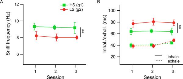
Each marker represents the session mean of median values from a group of rats (n=3 rats per group). Error bars are SEM. Vertical lines with asterisks represent significant differences between the two groups. A) Mean instantaneous respiratory frequency derived from the length of each respiratory cycle (inhalation + exhalation). B) Inhalation (solid lines) and exhalation (dashed lines) means. The frequency difference shown in (A) was driven by a difference in inhalation duration between the two groups. Exhalation durations did not vary across groups. ** p<0.01.

Volume and flow estimates were also calculated from the rsEMG signal. There were no significant differences between groups or across sessions for these two measures when all of the first four inhalations were pooled for each odor sampling period (ANOVA volume: F_session(2,12)=0.1, p=0.90; F_group(1,12)=0.16, p=0.69; F_{session × group}(2,12)=0.21, p=0.81; flow: F_session(2,12)=0.17, p=0.84; F_group(1,12)=0.07, p=0.80; F_{session × group}(2,12)=0.45, p=0.65).

Single-inhalation analysis

Additional analyses were performed by looking separately at each of the first 4 inhalations during odor sampling (Figures 7 and 8). Session median inhalation and exhalation durations, volume and flow were calculated for each inhalation number, with the first inhalation defined as the first respiratory cycle whose inhalation-end event occurred while the nose was in the odor port. There were significant variations in inhalation durations across the 4 inhalations, with the first two inhalations typically shorter than the later ones, particularly in session 1, and as with analysis on all sniffs, LS-detecting rats inhaled longer than HS-detecting rats (Figure 7A; session 1 ANOVA: F_inhal#(3,16)=4.84, p=0.014, η²=0.40; F_group(1,16)=4.78, p=0.044, η²=0.13; F_{inhal# × group} (3,16)=0.35, p=0.79;session 2 ANOVA: F_inhal#(3,16)=4.32, p=0.021, η=0.34; F_group(1,16)=8.53, p=0.01, η²=0.23; F_{inhal# × group}(3,16)=0.13, p=0.94; session 3 ANOVA: F_inhal#(3,16)=2.26, p=0.12; F_group(1,16)=4.14, p=0.059, η²=0.15; F_{inhal# × group} (3,16)=0.16, p=0.92).

Figure 7. Inhalation durations in single-inhalation analysis during odor sampling.

Each trace represents a group (n=3 rats per group), and each number on the horizontal axis is a (consecutive) inhalation number, starting with the first inhalation within the odor port. Values shown are means of medians. Error bars are SEM. Horizontal bars with asterisks represent significant differences across inhalations; vertical bars represent differences between groups. All plots contain data from odor set A (HS- or LS-detecting rats). A: Mean duration of inhalations. i,ii) In sessions 1 and 2, duration varied significantly across inhalations, and LS-detecting rats inhaled longer than HS-detecting rats. iii) In session 3 the rat group difference decreased (p<0.1), and there was no longer a difference across inhalations. Curves represent group means of individual rats' medians for all attempts. B: Differences in inhalation duration in A depended on two different portions of the inhalation (curves calculated using all trials). The portion before the inhalation peak (solid curves) was shorter but LS-detecting rats inhaled longer in this portion. The portion after the peak (dashed curves) showed variation across inhalations in session 3. ** p<0.01, * p<0.05.

Figure 8. Inhalation volume and flow estimates in single-inhalation analysis during odor sampling.

Each trace represents a group (n=3 rats per group), and each number on the horizontal axis is the inhalation number during odor sampling. `pre' and `post' refer to the periods used for normalizing the measures, corresponding to prior to and after odor sampling respectively (see methods). Values shown are means of medians. Error bars are SEM. Horizontal bars with asterisks represent significant differences across inhalations; the vertical bar in session 3 represents differences between groups. A) Inhalation volume was the same for both groups in each session and did not vary across inhalations. B) Inhalation flow varied across inhalation cycles in all three sessions, and in session 3 LS-detecting rats used lower flows than HS-detecting rats.

Previous studies have shown that the initial part of the inhalation is associated with tidal volume more than the latter (Eldridge and Eldridge, 1971). Therefore, we further broke down the inhalation period by examining the duration from the start of inhalation to the peak (local maximum) of EMG activity and the peak to the end of inhalation separately. We found that the difference in inhalation duration between HS- and LS-detecting rats is mirrored by a similar difference in the first part of the inhalation (before the peak) in all three sessions (Figure 7B; ANOVA: session 1- F_group(1,16)=8.37, p=0.011, η²=0.27; session 2- F_group(1,16)=13.62, p=0.002, η²=0.45; session 3- F_group(1,16)=5.93, p=0.027, η²=0.23). We did not find significant differences between LS- and HS-detecting groups for the second portion of the inhalation (although there was a marginal effect in session 2), but there was a significant increase in the duration of the late portion of the inhalation over the four inhalations in session 3, and marginal effects in sessions 1 and 2, which matches the shape of the total inhalation duration curves (Figure 7B; ANOVA: session 1- F_sniff(3,16)=2.99, p=0.062, η²=0.33, F_group(1,16)=1.64, p=0.218, F_{sniff × group}(3,16)=0.15, p=0.93; session 2- F_sniff(3,16)=2.98, p=0.063, η²=0.30, F_group(1,16)=4.34, p=0.053, η²=0.15, F_{sniff × group}(3,16)=0.04, p=0.99; session 3- F_sniff(3,16)=5.19, p=0.011, η²=0.46, F_group(1,16)=2.06, p=0.170, F_{sniff × group}(3,16)=0.13, p=0.94).

To analyze our estimates of inhalation volume and flow, we normalized them as described in the methods, and calculated the medians for each inhalation number, session and rat. There were no differences in volume across inhalations or between groups in any session (Figure 8A; ANOVAs: session 1- F_inhal#(3,16)=0.79, p=0.51, F_group(1,16)=0.56, p=0.46, F_{inhal# × group}(3,16)=0.07, p=0.98; session 2- F_inhal#(3,16)=0.19, p=0.90; F_group(1,16)=2.06, p=0.17, F_{inhal# × group}(3,16)=0.12, p=0.95; session 3- F_inhal#(3,16)=0.10, p=0.96; F_group(1,16)=0.05, p=0.82; F_{inhal# × group}(3,16)=0.07, p=0.98). Flow varied as a function of inhalation number in all sessions, and between rat groups in session 3, when both groups performed the discrimination at high and comparable levels. In session 3, LS-detecting rats used lower flows than HS-detecting rats, and this is more pronounced in the first two inhalations (Figure 8B; ANOVAs: session 1-F_inhal#(3,16)=4.98, p=0.013, η²=0.47, F_group(1,16)=0.02, p=0.90, F_{inhal# × group}(3,16)=0.33, p=0.81; session 2- F_inhal#(3,16)=3.80, p=0.031, η=0.48; F_group(1,16)=0.02, p=0.89, F_{inhal# × group}(3,16)=0.07, p=0.98; session 3- F_inhal#(3,16)=7.04, p=0.003, η=0.48; F_group(1,16)=5.88, p=0.028, η²=0.13; F_{inhal# × group}(3,16)=0.36, p=0.78). This analysis indicates that 13% of the deviation of the flow estimate from the grand mean can be ascribed to the rat's belonging to a given group, that is, to the sorption of the target being detected. About 48% of the deviation can be attributed to the inhalation number.

DISCUSSION

We addressed whether rats modify sniffing behavior during the detection of a low- vs. high-sorptiveness odorant in binary mixtures. This question stems directly from a need to examine empirically some of the consequences of Schoenfeld and Cleland's zonation hypothesis, which was based on numerous lines of evidence but had not been tested in behaving animals. It is worth citing here the original formulation of the hypothesis: “We suggest that the motor regulation of sniffing behavior is substantially utilized for purposes of `zonation' or the direction of odorant molecules to defined intranasal regions and hence toward distinct populations of receptor neurons, pursuant to animals' sensory goals” (Schoenfeld and Cleland, 2006). Regarding the specific role of odorant sorptiveness in the process, they further explained: “…behavioral variations in sniffing will deposit odorants in predictable distributions along the inspiratory path, as a function of odorant sorptiveness, enabling animals to achieve particular sensory goals by actively regulating the motor parameters.”

To test the zonation hypothesis, we designed a Go/No-Go task that required rats to detect the presence of a single odorant -the target- in binary mixtures. We tested two groups of rats in parallel, challenging each with a target of high- (HS) or low-sorptiveness (LS), repeating the task across three sessions. Crucially, our task relied on detecting a single odorant in a binary mixture background. This is a better scenario to test the hypothesis than monomolecular odorant discriminations, because it is in the more complex situation of mixtures where the chromatographic separation abilities of the system are being challenged. Simultaneously with the discrimination task, we monitored rats' sniffing via the diaphragm EMG, which has been shown to be a very reliable measure of relative airflow during respiration (Katz et al., 1962; Eldridge and Eldridge, 1971; Lopata et al., 1976; Platt et al., 1998).

We found that rats' performance in detection depended critically on the target odorant sorptiveness (Figure 2a, b). This shows that odorant sorption is an important factor in rats' ability to disambiguate odor stimuli and, more generally, that the physical properties of both the odorants and the mucosa contribute to the ease with which odorants can be detected, somewhat independently of the odorant's properties as a ligand of an olfactory receptor. Even though LS-detection was harder, rats nonetheless managed to discriminate at levels comparable to their HS-detection, only requiring more sessions and using different inhalation strategies to do so. These results are consistent with a study in humans, based on natural fluctuations in nasal airflow, which showed them more likely to identify a LS odorant in a mixture when delivered at low flow rates (Sobel et al., 1999).

We found, consistent with other studies, no changes in overall sampling duration according to discrimination difficulty (Figure 2c; Uchida and Mainen, 2003; Rinberg et al., 2006; Frederick et al., 2011). Although the rats did not adjust sampling duration, longer sniffing bouts and more sniffs were associated with increased performance in the lower-performing LS-detecting rats relative to HS-detecting rats (Figures 5 and 6). For odor set B, which for both groups was the second odor set learned, HS-detecting (group 2) rats sampled longer than LS-detecting (group 1) rats (Figure 2C.ii), but HS-detecting rats needed much less sampling time to make a correct decision, as did the HS-detecting (group 1) rats for odor set A (Figure 3). We suspect that the sampling duration difference in odor set B may have something to do with switching the target type they were tracking from odor set A to odor set B.

The zonation model predicts that increases in flow enhance the relative strength of a HS-evoked signal with respect to its LS counterpart, and that decreases in flow produce the opposite effect (Schoenfeld and Cleland, 2006). This relies on expression of receptors that are more sensitive to HS odorants in zones of the nasal passageways relatively early in the path of inspiratory airflow, and those more sensitive to LS odorants relatively late in the path (Freitag et al., 1998; Malnic et al., 1999; Mezler et al., 2001; Zhang and Firestein, 2002). Thus, a behavioral prediction of this hypothesis is that comparable levels of high performance between rat groups detecting targets of different sorptiveness should be accompanied by different sniffing strategies, each optimized to a particular target type. When comparing sniffing modes between rat groups, we found that LS-detecting rats showed longer individual inhalations than HS-detecting rats in sessions 1 and 2 and to a lesser extent in session 3 (Figure 7A). These longer inhalations reflected a longer rise to the peak of inhalation (Figure 7B), which means that the respiratory muscle's speed of contraction must have been actively modulated to achieve the observed differences.

The two groups did not differ in volume of individual inhalations, nor did volume change significantly across inhalations (Figures 8B, 8A). Flow varied significantly across inhalations in every session, producing a pattern of fast flow for the first two inhalations followed by decreasing airflow in inhalations 3 and 4. The two groups used the same flow strategies in sessions 1 and 2. Only in session 3, when performance was high and comparable between rat groups, did the rat groups differ in their inhalation flows. LS-detecting rats displayed lower flows than HS-detecting rats, something that was not observed when LS-detecting rats were not detecting the target well, i.e., during sessions 1 and 2 (Figure 8B). These concomitant changes in flow strategies and performance are in line with the chromatographic and zonation hypotheses.

Although we detected that the rat groups' sniff strategies differed depending on the target's sorptiveness, we were not able to evaluate which group adjusted sniff strategies. One interpretation is that the high instantaneous respiratory frequencies for HS-detecting rats, as compared to other studies, suggests that increasing frequencies and flow favors HS odorants (Schoenfeld and Cleland, 2006). Another interpretation is that since both groups showed variability in sniff parameters across sessions they both changed their sniff strategies to accommodate their targets.

Why did group differences in sniffing parameters change from inhalation duration in sessions 1 and 2 to flow in session 3? The larger inhalation durations for LS-detecting rats in sessions 1 and 2, respectively, with the same flow rate for the two groups would increase the duration of the odor sample and enhance perception of the harder to detect LS target, allowing the rats to pay attention to the stimulus feature that is key for discrimination. Returning to the analogy with the visual system, this longer odor sample could be a way to focus on a barely visible feature or to saccade more precisely to the zone of the perceptual field where a small spot (the LS target) is located. Once the feature is identified, the target is easier to find, and the extended sampling time is no longer needed. The difference is converted to flow in session 3 to easily identify a known target.

Might factors other than sorption explain these results? If we examine other physical properties of these odorants that might affect both performance and sniffing, we find that none account for the results as completely as sorption. Vapor pressure is a measure of volatility and has been linked in other studies to sensitization or short term learning and to sampling duration (Lowry and Kay, 2007). In odor set A the two targets have nearly identical vapor pressures. In odor set B, the vapor pressures are slightly different, but the difference is small given the logarithmic scale on which behavioral effects occur, and a higher vapor pressure should make the LS odorant easier to detect than the HS odorant. Another molecular feature that may affect detection of odorants is molecular weight, and these values are in the opposite direction for LS vs. HS odorants in odor sets A and B. We examined a list of molecular descriptors for each of the four targets and none of them differed in the same direction and similar magnitude across the two pairs, except for the sum of conventional bond orders (Table 6); we were unable to understand how this sum might contribute to odorant detection, but it is possible that it does, or that other molecular features may drive these effects. However, the most parsimonious explanation of the behavioral and respiratory effects associated with our odor sets is the difference in sorptiveness of the targets in each pair.

Table 6.

Molecular descriptors of the 4 target odorants used (odor sets A and B, HS and LS targets for each).

		LS	HS	LS	HS
Descriptor		ethylbenzene	cyclooctane	octane	isopropanol
sorptiveness	Kaw	8×10-3	7×10-4	3.38	1×10-5
vapor pressure	VP	7.71	7.85	12.23	7.2
molecular weight	MW	106.18	112.24	114.26	74.14
average MW	AMW	5.9	4.68	4.39	4.94
sum Van der Waals volumes	Sv	10.99	12.78	13.38	7.5
sum atomic Sanderson electronegativities	Se	17.42	23.07	24.95	14.75
sum of atomic polarizabilities	Sp	11.81	14.09	14.85	8.26
sum of Kier-Hall electrotopological states	Ss	15.17	12	13	12.83
mean Van der Waals volume	Mv	0.61	0.53	0.51	0.5
mean atomic Sanderson electronegativitiy	Me	0.97	0.96	0.96	0.98
mean atomic polarizability	Mp	0.66	0.59	0.57	0.55
mean electrotopological state	Ms	1.9	1.5	1.63	2.57
#atoms	nAT	18	24	26	15
#non-H atoms	nSK	8	8	8	5
#bonds	nBT	18	24	25	14
#non-H bonds	nBO	8	8	7	4
#multiple bonds	nBM	6	0	0	0
sum conventional bond orders (H-depleted)	SCBO	11	8	7	4
aromatic ratio	ARR	0.75	0	0	0
#rings	nCIC	1	1	0	0
#circuits	nCIR	1	1	0	0
#rotatable bonds	RBN	1	0	5	1
rotatable bond fraction	RBF	0.056	0	0.2	0.071
#conjugated bonds	nAB	6	0	0	0
#H	nH	10	16	18	10
#C	nC	8	8	8	4

Shaded row for “sum conventional bond orders” shows differences that have a similar pattern and large magnitude as the sorptiveness differences. Descriptors omitted for which there was little or no representation across odorants. Molecular features data from MOLE db (Ballabio et al., 2009).

We conclude that detecting the presence or absence of HS-odorants in binary mixtures may be easy for rats because of the physical properties of the mucosa, and that rats do adjust sniffing parameters, such as duration and flow of inhalation, to targets of differing sorption qualities when sniffing the very same binary mixtures. The strategy may be necessary but not sufficient for solving the problem, and adjusting sniff parameters may only accomplish part of the task. Central processes should also account for some part of the performance increases. Future studies should be aimed at understanding the role and control of other respiratory muscles and the ways in which this response interacts with central processes.

REFERENCES

- Adrian ED. Sensory discrimination - with some recent evidence from the olfactory organ. British Medical Bulletin. 1950;6:330–332. doi: 10.1093/oxfordjournals.bmb.a073625. [DOI] [PubMed] [Google Scholar]
- Ballabio D, Manganaro A, Consonni V, Mauri A, Todeschini R. Introduction to MOLE DB - on-line molecular descriptors database. MATCH, Communications in Mathematical and in Computer Chemistry. 2009;62:199–207. [Google Scholar]
- Berg RW, Kleinfeld D. Rhythmic whisking by rat: retraction as well as protraction of the vibrissae is under active muscular control. Journal of neurophysiology. 2003;89:104–117. doi: 10.1152/jn.00600.2002. [DOI] [PubMed] [Google Scholar]
- Eldridge L, Eldridge FL. Relationship between phrenic nerve activity and ventilation. American Journal of Physiology. 1971;221:535–543. doi: 10.1152/ajplegacy.1971.221.2.535. [DOI] [PubMed] [Google Scholar]
- Frederick DEE, Rojas-Libano D, Scott M, Kay LM. Rat behavior in go/no-go and two-alternative choice odor discrimination: differences and similarities. Behavioral Neuroscience. 2011;125:588–603. doi: 10.1037/a0024371. [DOI] [PMC free article] [PubMed] [Google Scholar]
- Freitag J, Ludwig G, Andreini I, Rossler P, Breer H. Olfactory receptors in aquatic and terrestrial vertebrates. J Comp Physiol A. 1998;183:635–650. doi: 10.1007/s003590050287. [DOI] [PubMed] [Google Scholar]
- Glasstone S, Lewis D. Elements of Physical Chemistry. D. van Nostrand Company; Princeton: 1960. [Google Scholar]
- Haynes WA. CRC Handbook of Chemistry and Physics. 2010. [Google Scholar]
- Hedges LV. Distribution theory for Glass's estimator of effect size and related estimators. Journal of Educational Statistics. 1981;6:107–128. [Google Scholar]
- Hentschke H, Stuttgen MC. Computation of measures of effect size for neuroscience data sets. Eur J Neurosci. 2011;34:1887–1894. doi: 10.1111/j.1460-9568.2011.07902.x. [DOI] [PubMed] [Google Scholar]
- Hornung DE, Mozell MM. Accessibility of odorant molecules to the receptors. In: Cagan RH, Kare MR, editors. Biochemistry of Taste and Olfaction. Academic Press; New York: 1981. pp. 33–45. [Google Scholar]
- Katz RL, Fink BR, Ngai SH. Relationship between electrical activity of the diaphragm and ventilation. Proc Soc Exp Biol Med. 1962;110:792–794. doi: 10.3181/00379727-110-27652. [DOI] [PubMed] [Google Scholar]
- Kent PF, Mozell MM, Murphy SJ, Hornung DE. The interaction of imposed and inherent olfactory mucosal activity patterns and their composite representation in a mammalian species using voltage-sensitive dyes. J Neurosci. 1996;16:345–353. doi: 10.1523/JNEUROSCI.16-01-00345.1996. [DOI] [PMC free article] [PubMed] [Google Scholar]
- Kepecs A, Uchida N, Mainen ZF. Rapid and precise control of sniffing during olfactory discrimination in rats. J Neurophysiol. 2007;98:205–213. doi: 10.1152/jn.00071.2007. [DOI] [PubMed] [Google Scholar]
- Kline RB. Beyond significance testing. American Psychological Association; Washington, DC: 2004. [Google Scholar]
- Konow N, Thexton A, Crompton AW, German RZ. Regional differences in length change and electromyographic heterogeneity in sternohyoid muscle during infant mammalian swallowing. Journal of applied physiology (Bethesda, Md : 1985) 2010;109:439–448. doi: 10.1152/japplphysiol.00353.2010. [DOI] [PMC free article] [PubMed] [Google Scholar]
- Lopata M, Evanich M, Lourenço R. The electromyogram of the diaphragm in the investigation of human regulation of ventilation. Chest. 1976;70:162–165. doi: 10.1378/chest.70.1_supplement.162. [DOI] [PubMed] [Google Scholar]
- Lowry CA, Kay LM. Chemical factors determine olfactory system beta oscillations in waking rats. Journal of Neurophysiology. 2007;98:394–404. doi: 10.1152/jn.00124.2007. [DOI] [PubMed] [Google Scholar]
- Mackay-Sim A, Shaman P, Moulton DG. Topographic coding of olfactory quality: odorant-specific patterns of epithelial responsivity in the salamander. J Neurophysiol. 1982;48:584–596. doi: 10.1152/jn.1982.48.2.584. [DOI] [PubMed] [Google Scholar]
- Malnic B, Hirono J, Sato T, Buck LB. Combinatorial receptor codes for odors. Cell. 1999;96:713–23. doi: 10.1016/s0092-8674(00)80581-4. [DOI] [PubMed] [Google Scholar]
- Mezler M, Fleischer J, Breer H. Characteristic features and ligand specificity of the two olfactory receptor classes from Xenopus laevis. J Exp Biol. 2001;204:2987–2997. doi: 10.1242/jeb.204.17.2987. [DOI] [PubMed] [Google Scholar]
- Moncrieff RW. The sorptive properties of the olfactory membrane. J Physiol. 1955;130:543–558. doi: 10.1113/jphysiol.1955.sp005426. [DOI] [PMC free article] [PubMed] [Google Scholar]
- Mozell MM, Jagodowicz M. Chromatographic separation of odorants by the nose: retention times measured across in vivo olfactory mucosa. Science. 1973;181:1247–1249. doi: 10.1126/science.181.4106.1247. [DOI] [PubMed] [Google Scholar]
- Mozell MM, Kent PF, Murphy SJ. The effect of flow rate upon the magnitude of the olfactory response differs for different odorants. Chem Senses. 1991;16:631–649. [Google Scholar]
- Platt RS, Hajduk EA, Hulliger M, Easton PA. A modified Bessel filter for amplitude demodulation of respiratory electromyograms. J Appl Physiol. 1998;84:378–388. doi: 10.1152/jappl.1998.84.1.378. [DOI] [PubMed] [Google Scholar]
- Rangayyan RM. Biomedical signal analysis. A case-study approach. IEEE Press - John Wiley; New York: 2002. [Google Scholar]
- Rinberg D, Koulakov A, Gelperin A. Speed-accuracy tradeoff in olfaction. Neuron. 2006;51:351–358. doi: 10.1016/j.neuron.2006.07.013. [DOI] [PubMed] [Google Scholar]
- Schoenfeld TA, Cleland TA. The anatomical logic of smell. Trends in neurosciences. 2005;28:620–627. doi: 10.1016/j.tins.2005.09.005. [DOI] [PubMed] [Google Scholar]
- Schoenfeld TA, Cleland TA. Anatomical contributions to odorant sampling and representation in rodents: zoning in on sniffing behavior. Chem Senses. 2006;31:131–144. doi: 10.1093/chemse/bjj015. [DOI] [PubMed] [Google Scholar]
- Scott JW, Brierley T, Schmidt FH. Chemical determinants of the rat electro-olfactogram. J Neurosci. 2000;20:4721–4731. doi: 10.1523/JNEUROSCI.20-12-04721.2000. [DOI] [PMC free article] [PubMed] [Google Scholar]
- Scott-Johnson PE, Blakley D, Scott JW. Effects of air flow on rat electroolfactogram. Chem Senses. 2000;25:761–8. doi: 10.1093/chemse/25.6.761. [DOI] [PubMed] [Google Scholar]
- Shafford HL, Strittmatter RR, Schadt JC. A novel electrode design for chronic recording of electromyographic activity. J Neurosci Methods. 2006;156:228–230. doi: 10.1016/j.jneumeth.2006.03.009. [DOI] [PubMed] [Google Scholar]
- Sobel N, Khan RM, Saltman A, Sullivan EV, Gabrieli JD. The world smells different to each nostril. Nature. 1999;402:35. doi: 10.1038/46944. [DOI] [PubMed] [Google Scholar]
- Strittmatter RR, Schadt JC. Sex differences in the respiratory response to hemorrhage in the conscious, New Zealand white rabbit. Am J Physiol Regul Integr Comp Physiol. 2007;292:R1963–9. doi: 10.1152/ajpregu.00494.2006. [DOI] [PubMed] [Google Scholar]
- Uchida N, Mainen ZF. Speed and accuracy of olfactory discrimination in the rat. Nature Neuroscience. 2003;6:1224–1229. doi: 10.1038/nn1142. [DOI] [PubMed] [Google Scholar]
- Verhagen JV, Wesson DW, Netoff TI, White JA, Wachowiak M. Sniffing controls an adaptive filter of sensory input to the olfactory bulb. Nature Neuroscience. 2007;10:631–639. doi: 10.1038/nn1892. [DOI] [PubMed] [Google Scholar]
- Yang GC, Scherer PW, Zhao K, Mozell MM. Numerical modeling of odorant uptake in the rat nasal cavity. Chem Senses. 2007;32:273–284. doi: 10.1093/chemse/bjl056. [DOI] [PubMed] [Google Scholar]
- Yarbus AL. Eye Movements and Vision. Plenum Press; New York: 1967. [Google Scholar]
- Youngentob SL, Mozell MM, Sheehe PR, Hornung DE. A quantitative analysis of sniffing strategies in rats performing odor detection tasks. Physiol Behav. 1987;41:59–69. doi: 10.1016/0031-9384(87)90131-4. [DOI] [PubMed] [Google Scholar]
- Zhang X, Firestein S. The olfactory receptor gene superfamily of the mouse. Nat Neurosci. 2002;5:124–33. doi: 10.1038/nn800. [DOI] [PubMed] [Google Scholar]