Functional Characterization of the Extra-Classical Receptive Field in Macaque V1: Contrast, Orientation, and Temporal Dynamics

Abstract

Neurons in primary visual cortex, V1, very often have extra-classical receptive fields (eCRFs). The eCRF is defined as the region of visual space where stimuli cannot elicit a spiking response but can modulate the response of a stimulus in the classical receptive field (CRF). We investigated the dependence of the eCRF on stimulus contrast and orientation in macaque V1 cells for which the laminar location was determined. The eCRF was more sensitive to contrast than the CRF across the whole population of V1 cells with the greatest contrast differential in layer 2/3. We confirmed that many V1 cells experience stronger suppression for collinear than orthogonal stimuli in the eCRF. Laminar analysis revealed that the predominant bias for collinear suppression was found in layers 2/3 and 4b. The laminar pattern of contrast and orientation dependence suggests that eCRF suppression may derive from different neural circuits in different layers, and may be comprised of two distinct components: orientation-tuned and untuned suppression. On average tuned suppression was delayed by about 25 milliseconds compared to the onset of untuned suppression. Therefore, response modulation by the eCRF develops dynamically and rapidly in time.

INTRODUCTION

Neurons in primary visual cortex, V1, very often have extra-classical receptive fields (eCRFs). The eCRF is defined as the region of visual space where stimuli cannot elicit a spiking response but can modulate the response of a stimulus in the classical receptive field (CRF). Determining the properties of the eCRF is important for understanding V1 activity under natural viewing conditions, where stimuli are rarely spatially restricted and the local image statistics (orientation, contrast) can vary across the scene. Response modulation of the CRF by stimulation of the surrounding eCRF of V1 neurons has been implicated in a variety of perceptual phenomena (Blakemore & Tobin, 1972; Allman et al., 1985; DeAngelis et al., 1994). Among these are figure-ground segregation (Lamme, 1995), contour integration (Li et al., 2006), signaling of object junctions (Sillito et al., 1995; Yazdanbakhsh and Livingstone, 2006), and motion contrast (Baker and Graf, 2010). The effects of eCRF modulation when the CRF is stimulated with different contrast levels depend on the stimulus conditions; facilitation, suppression, or some combination of the two has been reported (Levitt & Lund, 1997; Sengpiel et al., 1997;. Somers et al., 1998; Kapadia et al., 1999; 2000; Sceniak et al., 1999; 2001; Cavanaugh et al., 2002a,b; Sadakane et al., 2006; Ichida et al., 2007; Schwabe et al., 2010). We have investigated single-cell responses in V1 under conditions of moderate to strong CRF drive and stimuli covering large regions of the eCRF, when the eCRF modulation is predominantly suppressive (Sceniak et al., 1999; 2001; Levitt & Lund, 2002).

A principal aim of our research was to characterize the contrast sensitivity of the eCRF signal and relate it to the contrast sensitivity of the CRF. We found that the contrast for half-maximal response, C₅₀, was lower for eCRF suppression than for CRF excitation. However, the higher contrast sensitivity of the eCRF compared to the CRF was not the same in all cortical layers: the difference in C₅₀ between eCRF and CRF was greatest in the cortico-cortical output layers 2/3.

Studies of orientation selectivity indicate that there are two components of suppression: one that is untuned for orientation and local to the CRF and another that is orientation-selective and extending into the eCRF (Xing et al., 2005; Xing et al., 2011). In our study of the eCRF, we found that tuned suppression was most significant in layers 2/3 and 4b, while untuned suppression was observed in all layers. Response dynamics measurements revealed that the onset time of tuned suppression was delayed by about 25 milliseconds with respect to the untuned component.

MATERIALS AND METHODS

Preparation and recording

Adult male old-world monkeys (M. fascicularis) were used in acute experiments in compliance with National Institutes of Health and New York University Animal Use Committee regulations. The animal preparation and recording were performed as described in detail previously (Hawken et al., 1996; Ringach et al., 2002; Xing et al, 2005). Anesthesia was induced with ketamine (5-20 mg/kg, i.m.) and initially maintained with isofluorane (1-3%) for venous cannulation and intubation. Then anesthesia was continued with sufentanil citrate (6-18 μg/kg/h, i.v.) for the remainder of the surgery and recording. Once surgery was completed, muscle paralysis was induced and maintained with vecuronium bromide (Norcuron, 0.1 mg/kg/h, i.v.). Heart rate, EKG, blood pressure, expired CO₂, and EEG were continuously monitored to ensure the maintenance of anesthesia. Ophthalmic atropine sulfate (1%) was administered to the eyes to dilate the pupils at the start of the experiment. For the duration of the experiment, the eyes were protected by clear, gas-permeable contact lenses and application of gentamicin sulfate (3%), a topical antibiotic solution. Fixation rings (Duckworth and Kent) were used to minimize eye movements in most experiments and, when used, an ophthalmic anti-inflammatory agent (TobraDex) was also applied.

Foveae were mapped on to a tangent screen using a reversing ophthalmoscope and the receptive fields of isolated neurons were mapped in relation to the foveae. Extracellular activity was recorded using glass-coated tungsten microelectrodes (Merrill and Ainsworth, 1972) that were advanced through a craniotomy over occipital cortex using a motorized stepping microdrive (Narishige). Individual spikes were discriminated via custom software running on a Silicon Graphics O2 and were time stamped with 0.1 ms resolution. Single unit activity was identified by a fixed action potential shape and an absolute refractory period between individual spikes.

After the completion of each electrode penetration, 3-5 small electrolytic lesions (3 μA for 3 s) were made at separate locations along the electrode track. At the end of the experiments, the animals were deeply anesthetized with sodium pentobarbital (60 mg/kg, i.v.) and transcardially exsanguinated with heparinized lactated Ringer, followed by 4 liters of chilled fresh 4% paraformaldehyde in 0.1 M phosphate buffer (pH 7.4). The electrolytic lesions were located in the fixed tissue and electrode tracks were reconstructed to assign the recorded neurons to cortical layers (as in Hawken et al., 1988).

Characterization

Each single neuron was stimulated monocularly through the dominant eye (with the non-dominant eye occluded). The steady-state response to drifting gratings was determined to provide an initial characterization. The initial measurements were orientation tuning, spatial and temporal frequency tuning, contrast response with achromatic gratings and color sensitivity followed by area summation and annulus summation curves. Receptive fields were located at eccentricities between 1 and 6 deg. Stimuli were displayed at a screen resolution of 1024x768 pixels and a refresh rate of 100 Hz. The stimuli were presented on either a Sony Trinitron GDM-F520 CRT monitor or an Iiyama HM204DT-A CRT monitor with mean luminances of 90-100 cd/m² and 60 cd/m², respectively. The monitors’ luminance was calibrated using a spectroradiometer (Photo Research PR-650) and linearized via a lookup table in custom software. Each eye was optimally refracted for the 115 cm monitor viewing distance using external lenses.

Stimuli

Determination of the CRF and eCRF

Prior to quantitative measurements of the response, the receptive field center for each neuron was determined by hand-mapping the minimum response field using the smallest patch of optimal grating that produced a response from the cell (typically around 0.1 degree radius). The size of the optimal stimulus patch was determined by measuring the response as a function of the radius of a circular patch (area summation) that windowed the optimal grating (Fig. 1B). The border of the eCRF region was determined in a second experiment using an expanding annulus, where the response was measured as a function of the radius of the mean grey region in the center of a square patch of grating that was 8 deg on a side (Fig. 1C). As the central grey patch’s radius increased then the width of the outer grating region decreased correspondingly. This experiment was used to determine the size of the inner diameter of the eCRF region – the region where no response was elicited from the surround region when the center region was masked by a grey screen (as in Cavanaugh et al., 2002a), marked by the vertical arrow in Fig. 1C. Beyond this region was the extra-classical receptive field. We used the data collected from these two area summation experiments to determine the size of the stimuli in the subsequent experiments. The radius of the stimulus for the CRF was chosen to be the radius that evoked the peak response in the area summation experiment, shown by the vertical arrow at a radius of 0.75 deg for the example neuron in Fig. 1B. The eCRF stimulus was an annular region with an 8 degree by 8 degree square outer extent and an inner radius derived from the annular summation experiment, shown by the vertical arrow at a radius of 1.0 deg in Fig. 1C. The outer diameter of the CRF stimulus region was always smaller than the inner diameter of the eCRF stimulus region. The annular region between these two stimulus areas was mean grey.

Fig 1.

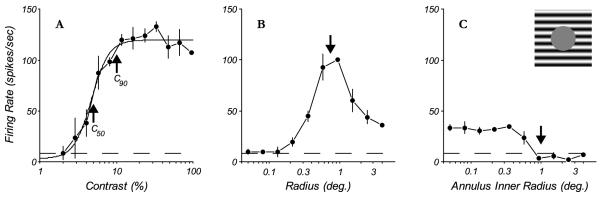
Contrast-response and size tuning for a complex cell. A: the response as a function of contrast for a grating of the optimal orientation, spatial and temporal frequency and drift direction, presented in a circular window that was the optimal size for the classical receptive field (CRF). The solid line is the best-fitting Naka-Rushton function. The arrows show the contrast eliciting 50% (C₅₀) and 90% (C₉₀) of the maximum response of the neuron, which were the contrasts used for subsequent contextual experiments. The dashed line indicates the spontaneous firing rate. B: the response as a function of the radius of the circular window containing an optimal grating as described above in (A). The arrow shows the smallest window radius eliciting the peak response of the neuron, which is the size of the central patch used in subsequent contextual experiments. C: a full field optimal grating was presented that included a central grey circular region, where the radius of the central region varied from 0 to 4 degrees, in 1/2 octave steps. The arrow shows the smallest radius of central blank grey region that elicited no response from the neuron. This size was used as the inner radius of stimuli presented to the extra-classical receptive field (eCRF) and the outer radius of the grey annulus separating stimuli in the CRF from the eCRF (see the configuration in Fig. 2B, C).

Contrast response function

A contrast response function for the CRF was obtained for a range of contrasts (Fig. 1A) with an optimal stimulus in the CRF alone, surrounded by uniform grey (Fig. 2A). Contrast ranged from 2 – 99% in 0.5 octave steps. Presentation was in an ascending order of contrast to minimize adaptation and hysteresis effects (Bonds 1991); a blank period, equal in duration to the stimulus presentation duration, was interleaved between each stimulus presentation.

Fig. 2.

CRF and eCRF contrast-response function comparison. A: stimulus configuration for CRF alone, where a central patch of grating optimized in orientation, spatio-temporal frequency, drift direction (red arrow) and size for the individual neuron. B: stimulus configuration for CRF in the presence of a collinear eCRF, a central patch of grating as in (A), simultaneously presented with a grating in the eCRF at the same spatiotemporal frequency and orientation. There was a small annular grey region that separated the center patch and the grating in the eCRF. The radius of the center patch was the optimal size for the CRF. The outer radius of the grey annulus was the size chosen from the expanding grey disc experiment where there was no response marked by the arrow in Fig. 1C. C: stimulus configuration for CRF in the presence of an eCRF stimulus oriented orthogonally to the central grating. For (B) and (C), the gratings in the eCRF were presented at a range of contrasts, from 5% to 80%, in octave steps. D: the contrast-response function for the CRF. E: contrast suppression function from the eCRF in response to collinear eCRF stimuli. F: contrast suppression function for orthogonal eCRF stimuli. In D-F the closed circles and error bars indicate mean ± 1 s.d. Lines are best fits of the Naka-Rushton function to the data. For comparison of parameters between conditions, estimates of parameter distributions were achieved by repeated fitting to bootstrap samples of the data. G: distributions of C₅₀ H: distributions of exponent parameter, for CRF (black), collinear eCRF (red), and orthogonal eCRF (blue).

To measure contrast effectiveness of the eCRF, an optimal stimulus, at a contrast eliciting 90% of the neuron’s maximum response (C₉₀), was presented to the CRF simultaneously with gratings confined to the eCRF. For some neurons additional experiments were also run with a contrast eliciting 50% of the maximal response for the CRF stimulus (C₅₀). Gratings in the eCRF had the same spatial and temporal frequency as the grating in the CRF and were presented at collinear and orthogonal orientations with respect to the central stimulus patch, across ranges from 5 – 80% luminance contrast in octave steps. Stimuli for eCRF experiments were presented for 0.5-1 second. Analysis of temporal dynamics was restricted to the first 0.5 seconds of stimulus presentation. Contrast response functions for eCRF suppression were obtained by converting observed firing rates for each stimulus condition to percent response suppression, relative to the control condition of a 0% contrast stimulus in the eCRF. Thus, the suppression index (SI) at a given eCRF stimulus contrast C was defined as:

$$\mathrm{SI}\left(C\right)=100\ast [R_0-R_C]∕R_0.$$

Data analysis

Responses were the mean firing rate (F0) taken over the duration of the stimulus presentation for complex cells and the amplitude of the first harmonic response (F1) for simple cells.

Contrast response function comparison

To compare the contrast sensitivities of the CRF and eCRF we compared estimates of the parameters of the Naka-Rushton function (Naka and Rushton, 1966) for half maximal sensitivity (C₅₀) and exponent (N) using the following equation:

$$R\left(C\right)=R_{\max }\times \left[\frac{C^N}{(C^N+C_{50}^N)}\right]+M$$

where R_max is the maximal response, M is the spontaneous response rate, and C is the stimulus contrast. For individual cells, parameter estimation was achieved by a large number of repeated fits to bootstrapped samples of the data. Specifically, for each stimulus condition a new response was generated for each contrast by randomly drawing the same number of samples as in the original experiment from the data, with replacement. This procedure was done for each contrast and parameters were determined through Naka-Rushton fits to each generated dataset (least squares fit using the Matlab function lsqcurvefit). The distribution of these parameter estimates in individual neurons was measured by repeating this process a large number of times (10⁵).

Significance testing of differences in parameters between the individual CRF and eCRF contrast response functions was conducted by repeated comparisons of draws from the two distributions a large number of times (10⁵). A comparison is reported as significant where one parameter is greater at least 95% of the time (p<0.05).

Response latency

Analysis of the temporal dynamics of modulation from the eCRF was conducted on a population of 68 complex cells. Simple cells modulate their responses in time to presentation of a drifting sinewave grating, and the phase of the modulation could potentially obscure the dynamics we were attempting to measure from the eCRF such as response onset; thus, analysis was confined to a subpopulation of complex cells. This population was selected to be complex cells with sufficient peak firing rates (> 10 spikes/sec) and at least 15% response suppression (for the most effective eCRF stimulus).

Responses to all stimulus conditions were aligned to each neuron’s CRF response onset latency, the time of response onset to an optimal grating in the CRF. To estimate CRF response onset latency, we first measured the background firing rate (mean and standard deviation) in the first 25 ms after stimulus onset, before signals were likely to have reached the primary visual cortex. We estimated the neuron’s response onset latency to be the earliest time point in the CRF response at which the instantaneous firing rate increased to 2 standard deviations above the background mean. Results were similar when we used a different measure of response onset latency: the first time at which the response exceeded 10% of each neuron’s maximum instantaneous firing rate.

To determine the onset latency of response suppression from a stimulus in the eCRF, we compared the cumulative spike counts over the stimulus presentation for two conditions: one in which an isolated stimulus was in the CRF and the other in which CRF and eCRF were co-stimulated. Cumulative spike count distributions at each time point for each stimulus condition were generated by repeated bootstrap resampling (with replacement) of the spike trains to repeated presentations of the stimuli. Suppression onset latency to a stimulus in the eCRF was determined to be the earliest time at which the cumulative spike count for the eCRF condition was significantly lower than the CRF alone condition (p<0.05) and remained lower for the following 20 ms. Results were similar when an alternate method of estimating suppression onset latency was used (the first time point at which the eCRF produced 5% of the total suppression observed over the entire stimulus presentation).

RESULTS

The activity of one hundred and fourteen neurons was recorded to investigate eCRF modulation. Here we report on three factors that are important for understanding how suppression may derive from different neural circuits in different layers. First we report on the contrast and orientation dependence of eCRF suppression across the whole population of V1 neurons. Next we show the laminar variation of suppression and determine the relationship between contrast sensitivity of the eCRF and CRF across layers. Third the interrelationship between eCRF stimulus properties and temporal response dynamics is investigated to provide further links to cortical circuits.

Contrast and orientation dependence of eCRF suppression

CRF visual characteristics

First we determined the visual properties of the CRF of each neuron. Measurements were made in the CRF of the orientation tuning, spatial and temporal frequency tuning, contrast response (Fig. 1A) and color sensitivity, as well as area summation using an expanding circular patch (Fig. 1B) and an expanding blank disk on a full field grating background (Fig. 1C). The contrast that evoked about 90% of the maximal response (C₉₀, Fig. 1A, right arrow) was chosen for subsequent experiments where stimulus-driven spike responses in the CRF were modulated by the eCRF under different conditions of eCRF stimulation. Some additional experiments also used the contrast evoking 50% of the maximal response in the CRF (C₅₀, Fig. 1A, left arrow). For this example neuron, the stimulus patch presented to the CRF had a radius of 0.75 degrees and the inner radius for the eCRF stimulus was 1.0 degree, as determined from area and annular summation measurements (Fig. 1B-C). We confined all of our eCRF probe stimuli to the region of the visual field between this inner radius and the outer border of an 8 × 8 degree square.

One of the goals of the experiments was to compare the contrast dependence of the response in the CRF with the contrast dependences of eCRF suppression. We first measured the contrast response of the CRF alone (Fig. 2A). Estimates of the contrast where the response reaches its half maximum (C₅₀), the exponent N, and maximal response (R_max) were obtained by fitting a Naka-Rushton function (Naka & Rushton, 1966) to the data (Fig. 2D, black curve).

eCRF contrast response

The contrast dependence of the eCRF modulation was determined by measuring the response suppression of CRF stimulation as a function of contrast presented in the eCRF. For an example neuron, as contrast of the collinear stimulus in the eCRF was increased, the strength of suppression increased, from around 40% response suppression for 5% contrast in the eCRF to 80% response suppression for 20 – 80% contrast (Fig. 2E). The strength of suppression for an orthogonal stimulus in the eCRF (Fig. 2F) was usually about half of the suppressive strength of the collinear stimulus (compare Fig. 2E-F). Nonetheless it is clear that the contrasts where suppression was first evident were lower than the contrasts required to evoke a response from the CRF (Fig. 2D).

The Naka-Rushton function also was used to fit the data for suppression-strength as a function of contrast in the eCRF (Fig. 2E-F). Estimates of the parameters (C₅₀, exponent N, and maximum percent suppression – R_max) that described the best-fitting function for each condition were used to compare the contrast dependences of the CRF and the eCRF for each neuron (as in Sadakane et al, 2006). We restricted our comparative analysis of fitted eCRF contrast-response functions to those neurons and stimulus orientations that exhibited significant eCRF suppression of at least 15% (94/114 collinear stimulus, 70/114 orthogonal stimulus). The reliability of the estimate of each fitted parameter was obtained from repeated fits to data samples drawn at random from the recorded response. The bootstrapped estimates of the fits were compared for each contrast response function fitted to responses from each neuron. The individual histograms shown in Fig. 2G-H are the parameter distributions from the fits to the single neuron’s contrast-response or contrast-suppression functions shown in Fig. 2D-F. (see Methods for more details of bootstrapping and significance testing). The estimate of C₅₀ for the CRF (Fig. 2G, black histogram) is 18.4% ± 1.0% (mean ± 1 s.d.) while the C₅₀ estimate for suppression from a collinear eCRF stimulus (Fig. 2G, red histogram) was 5.2% ± 0.5%. These values are significantly different (p < 0.001). The exponent N for the CRF was 4.7 ± 0.9 (Fig. 2H, black histogram) compared to 2.6 ± 1.2 (Fig. 2H, red histogram) for the collinear eCRF suppression. The exponents were also significantly different (p < 0.05). The estimates of C₅₀ and exponent for the orthogonal eCRF stimulus were 13.1% ± 3.1% and 1.6 ± 1.3 (Fig. 2G-H, blue histograms), respectively. There was less overlap in the estimates of the C₅₀’s for the three conditions (Fig. 2G) than for the exponents (Fig. 2H). It should be noted that in some cases, where there was a measurable suppression at the lowest contrast in the eCRF stimulus, the exponent was constrained at the lowest contrast because there is by definition no suppression at 0% eCRF contrast. If measurements had been made at lower eCRF contrasts the exponent, in some cases, might have been somewhat larger.

Across the population studied there was a range of relationships between the contrast dependence of the response from the CRF and the suppression to a collinear stimulus in the eCRF (Figure 3). For the majority of neurons, the collinear eCRF was either equally sensitive or more sensitive to contrast than the CRF; compare the first and second columns of the examples in Fig 3. The contrast where suppression was first evident was lower for the eCRF than for the contrast that first evoked a response from the CRF for the neurons in Figs. 3A-B, D-E and M-N, even though the maximum level of suppression was different across neurons. The second trend was that eCRF suppression was generally weaker for orthogonal stimuli compared to collinear stimuli (Levitt & Lund, 1997; Cavanaugh et al., 2002b; Shushruth et al., 2012; Shushruth et al., 2013) but still was evident in most cases (Fig. 3, compare the second and third columns). These two trends – higher eCRF than CRF contrast sensitivity, and stronger collinear than orthogonal suppression – were dominant across the population, as shown next.

Fig. 3.

Comparison of responses and suppression as a function of contrast in five neurons that show a range of CRF contrast response functions and suppression strengths from the eCRF. Each row represents a different neuron. The first column (A – M) shows contrast responses from the CRF for the example cells (mean ± 1 s.d.). Second (B – N) and third (C – O) columns show the percent suppression as a function of contrast from collinear- and orthogonal-oriented stimuli in the eCRF, respectively (mean ± 1 s.d.). Lines are best fits of the Naka-Rushton function to the data. Collinear suppression was generally stronger than orthogonal suppression, and C₅₀’s from eCRF were generally equal to or lower than C₅₀’s from CRF.

Population comparisons of CRF and eCRF

The semi-saturation contrast C₅₀ from the Naka-Rushton function-fit to the CRF and eCRF was used to provide a measure of the contrast sensitivity of each receptive field mechanism. Similarly R_max was used to compare suppression strength. In addition, the exponent (N) of the fitted function was compared between conditions.

For all neurons the parameters (C₅₀, R_max and exponent N) of the fits of the Naka-Rushton function to the contrast-responses in the CRF and contrast-dependent suppression in the eCRF, to both collinearly and orthogonally oriented stimuli, were tested for significance using a bootstrap procedure (see Methods). For the population the C₅₀ distribution for the eCRF had a lower mean than that of the CRF for both collinear (Fig. 4A) and orthogonal (Fig. 4B) orientations in the eCRF. The distribution of C₅₀’s for the eCRF collinear stimulus appears to be bimodal with one peak around 6% contrast and another between 20-30% contrast (Fig. 4A). The C₅₀ distribution of the CRF has a single peak at about 20% contrast. The CRF distribution’s single peak is consistent with the distribution of C₅₀ for the CRF of a larger population of cells recorded in our lab (see data in Fig. 6B of Clatworthy et al., 2003).

Fig. 4.

Comparison of C₅₀ values from CRF with eCRF. A: distribution of C₅₀ values from the Naka-Rushton function fitted to the contrast response of the CRF (black histogram) and contrast dependent suppression from the collinear orientation in the eCRF (grey). The arrows on the abscissa indicate the median values of each distribution. On average, eCRF C₅₀ values were lower than CRF C₅₀ values. B: histogram of CRF C₅₀ and orthogonal eCRF C₅₀. C: scatter plot of CRF and collinear eCRF C₅₀ values; points in red indicate a significant (p < 0.05) difference in the parameters. The majority of points lie above the unity line, indicating that within individual neurons eCRF C₅₀ values were significantly lower than CRF C₅₀ values. D: scatter plot of CRF and orthogonal eCRF C₅₀ values. Again, the majority of points lie above the unity line. E: scatter plot of C₅₀ values for both collinear and orthogonal eCRFs. For both orientations the eCRF C₅₀ distributions were centered around very low contrasts; however, there was no significant correlation between the two measures.

Fig. 6.

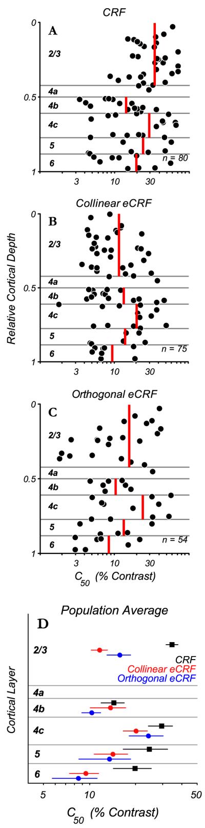
Contrast evoking half maximal response (C₅₀) of CRF and eCRF across cortical layers. Measures of C₅₀ are plotted for excitation from the CRF and suppression from the eCRF in relation to the cortical depth of recordings. Red vertical lines indicate mean values within each layer. A: laminar distribution of the C₅₀ parameter obtained from the best fitting Naka-Rushton function to the CRF contrast responses for each neuron. On average, the contrast eliciting half-maximal excitation from the CRF was around 20% for all layers and there was a trend for the lowest C₅₀’s to occur in layers 4b and 6. B: distribution of C₅₀ parameter values obtained for each neuron for eCRF suppression from collinear stimuli. Contrast sensitivity for suppression was high (C₅₀~10% contrast) across all layers, even in layers 2 and 3 for which the CRF had a low contrast sensitivity (A). C: the distribution of C₅₀ for suppression from orthogonal gratings in the eCRF. Even though orthogonal grating in the eCRF produced relatively weak suppression the sensitivities were higher on average than those for CRF excitation. D: summary plot of the average values for CRF (black squares) and eCRF C₅₀ (collinear – red circles; orthogonal – blue circles) across cortical layers (mean ±1 s.d.). eCRF C₅₀ values were lower than CRF values across all layers, with the largest differential in layers 2/3.

For around 76% (71/94) of the neurons tested, the eCRF C₅₀ for collinear suppression was lower than the CRF C₅₀ and for 33% (31/94) of neurons the C₅₀ was significantly lower (p < 0.05, red points above the equality line in Fig. 4C). Only 24% (23/94) of the neurons had eCRF C₅₀’s higher than the C₅₀ of the CRF and 4% (4/94) were significantly higher (p < 0.05, red points below the equality line in Fig. 4C). With an orthogonally-oriented stimulus in the eCRF the main effect also was for a lower C₅₀ for the eCRF than the CRF (Fig. 4D), with 27% (19/70) of neurons showing a significantly lower eCRF C₅₀ compared to 6% (4/70) of neurons where the eCRF C₅₀ was higher. While the C₅₀’s for both collinear and orthogonal eCRF suppression had similarly low values and contrast ranges, there was no significant correlation between the two measures (r = 0.18, p = 0.15, Fig. 4E). Overall the population comparison suggests that the eCRF was more sensitive to contrast than the CRF.

The magnitude of eCRF suppression of the center’s response depends on the orientation of the stimulus in the eCRF (Levitt & Lund, 1997; Cavanaugh et al., 2002b; Shushruth et al., 2012; Shushruth et al., 2013). For the population of neurons we studied, the R_max for collinear suppression was consistently greater than for orthogonal suppression (Fig. 5). Nonetheless there was little difference on average in the eCRF C₅₀ as a function of orientation. These results suggest that the contrast sensitivity of the suppressive component is not strongly dependent on suppression-strength or stimulus orientation in the eCRF. There was no discernible systematic relationship between the exponent of the contrast response function for the CRF and the exponent of the contrast dependency of suppression in the eCRF for either a collinear or orthogonal stimulus in the eCRF (data not shown).

Fig. 5.

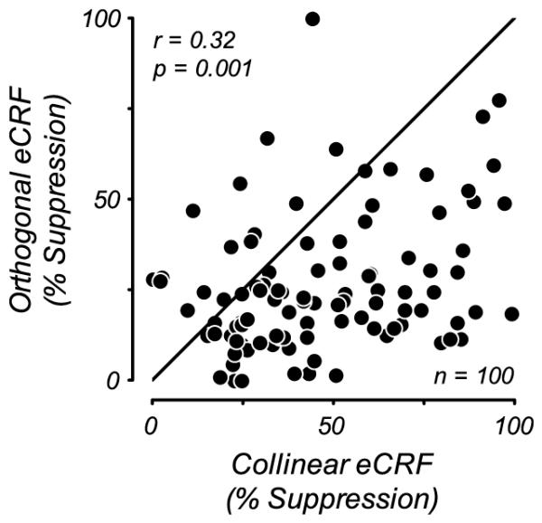
Orientation-dependent eCRF suppression strength. Scatter plot of the maximum strength of suppression from collinear and orthogonal stimuli in the eCRF. Suppression strength was defined as the percent suppression of CRF responses and was estimated as the R_max parameter from contrast-response function fits to eCRF suppression. There was a significant correlation between the strength of eCRF suppression for collinear and orthogonal stimuli (r = 0.32, p = 0.001). Nearly all points lie below the unity line, indicating that there was consistently stronger suppression from the collinear eCRF stimulus.

Mechanisms of CRF/eCRF contrast interactions

A further series of experiments was undertaken to probe the mechanisms of the substantial difference in half-maximal contrast, C₅₀, between the CRF and eCRF. Spatially segregated stimuli are often used in an attempt to drive the CRF and eCRF separately. However the underlying CRF and eCRF are not necessarily entirely separate in space and may indeed be partially or largely overlapping (as modeled by Sceniak et al., 2001; Cavanaugh et al., 2002a; Schwabe et al., 2006; among others). Thus, while an optimally-sized central stimulus engages no observable suppression in extracellular recordings, it may potentially provide sub-threshold drive to eCRF mechanisms. Therefore one potential explanation of the suppression from low-contrast stimuli presented to the eCRF, is that they activate a suppressive mechanism that has been brought near to its threshold by the CRF stimulus. The near threshold assumption predicts that lowering the contrast of a stimulus in the CRF should decrease the amount of suppression produced by a given stimulus in the eCRF. The model of Schwabe et al. (2010) predicts an increase in suppression for the midrange of CRF contrasts but is consistent with the near threshold predictions at low CRF contrasts where it predicts a decrease in suppression strength for a given eCRF stimulus.

To examine these predictions under our experimental conditions, we measured how the strength of suppression produced by given stimuli in the eCRF changed when the contrast of a stimulus in the CRF was lowered from C₉₀ to C₅₀. Suppression indices (SI) were significantly correlated between conditions with C₅₀ and C₉₀ contrasts in the CRF, for both collinear and orthogonal orientations in the eCRF (r=0.74, p < 0.00001, and r=0.46, p < 0.001, respectively). With collinear stimuli, the SI was significantly greater with a C₅₀ than with a C₉₀ stimulus in the CRF for both moderate to strong suppression, (SI>20%, p<0.00001) and weak suppression (SI<20%, p<0.0003, Wilcoxon signed rank test). With orthogonal eCRF stimuli that had an SI>20% at center contrast C₉₀, there was no significant change in SI when the CRF contrast was lowered from C₉₀ to C₅₀ (p = 0.11). However, for orthogonal SI<20% when center contrast = C₉₀, there was significantly stronger suppression when the contrast in the CRF was C₅₀ (p = 0.004). The results indicate that the strength of suppression increased somewhat when the contrast of a stimulus in the CRF was lowered to C₅₀. This result is consistent with the results of some previous studies (Levitt & Lund, 1997; Cavanaugh et al., 2002b; Schwabe et al. 2010).

As suppression from collinear eCRF stimuli was typically stronger than that from orthogonal eCRF stimuli, we also asked whether this difference in suppression strength was altered by a change in the contrast of the stimulus that drove the neurons’ classical receptive fields. Measures of the amount of orientation-tuned suppression (calculated as the difference in suppression indices between collinear and orthogonal eCRF stimuli) were made for all recorded neurons and all eCRF contrasts tested. Suppression to collinear stimuli remained strongest, whether or not the stimulus in the CRF was of relatively higher (C₉₀) or lower (C₅₀) contrast.

Furthermore, there was a significant correlation between tuned suppression at C₅₀ and at C₉₀ (r=0.41, p < 0.0001), demonstrating that the orientation-tuning of eCRF suppression persisted when the CRF was driven with a lower contrast. The strength of tuned suppression was significantly greater when the CRF was driven with C₅₀ contrast (p = 0.034, Wilcoxon signed rank test). Thus, both suppression from individual eCRF stimuli as well as orientation-selective suppression (measured across multiple stimuli) maintain or increase their efficacy when neurons’ CRFs are driven by stimuli of lowered luminance contrast, at least for the ranges of contrast examined in this study.

Laminar organization of eCRF suppression

Neurons in V1 show a diversity of modulation from their extra-classical receptive fields; some are entirely suppressed by spatially-extended stimuli and others summate over large areas without showing suppression. To understand how eCRF properties are generated in V1, it is important to know whether the variance in the population is partially due to differences in eCRF properties across cortical layers. Initially we determined how C₅₀ (of both CRF excitation and eCRF suppression) was distributed across cortical layers (Fig. 6). As there were no obvious trends within layers in our dataset, all statistical analyses were conducted by averaging over neurons within a given layer. However, a larger dataset could potentially reveal differences in contrast sensitivity within layer, such as between 4cα and 4cβ. In the majority of neurons in layers 2/3, the CRF was relatively insensitive to contrast (C₅₀ of 15% or greater) while about half of the neurons in layers 4b, upper 4cα and 6 had higher contrast sensitivities (Fig. 6A, red vertical lines indicate mean values within each layer). It is readily apparent that the C₅₀ values for the collinear eCRF suppression (Fig. 6B) were much lower than those for CRF excitation in layers 2/3. On average, contrast sensitivity for suppression was high (C₅₀ ~ 10%) across layers 2/3, 4b and 6; layer 4c was an exception. In layers 2/3, on average the eCRF C₅₀’s for collinear and orthogonal stimulus orientations (Fig, 6D red and blue circles respectively) were 2 to 3-fold lower than the average C₅₀ for the CRFs (black squares) which were relatively contrast-insensitive. The values for CRF and eCRF C50 differed significantly in layers 2/3 (p < 0.0001, Wilcoxon signed-rank test) but not in other cortical layers (p > 0.11). If eCRF properties are generated by intracortical connections, the differential contrast sensitivity between the eCRF and CRF suggests that neurons in cortical layers in which the CRF has higher contrast sensitivity (such as layers 4b and 4cα) provide a major source of the input to eCRFs of neurons in all cortical layers.

The magnitude of peak suppression in the eCRF was determined by the R_max parameter of the fitted contrast response functions – at both collinear (Fig. 3B-N) and orthogonal (Fig. 3C-O) orientations – and is shown as a function of cortical depth of the recorded neuron (Fig. 7A). Values near 100% indicate almost complete response-suppression to stimuli within the CRF and values near 0% indicate no modulatory effect. Results were similar when the measured suppression strength from the highest eCRF contrast tested was used instead of the R_max parameter (median difference ±1 s.d.: 1.9 ±6.0%). The eCRF collinear-stimulus suppression-strength (Fig. 7A, red lines: mean values) significantly varied across layers (p = 0.004, Kruskal-Wallis test) and was greatest in layers 2/3 and 4b, confirming results from previous studies (Sceniak et al., 2001; Shushruth et al., 2009). In addition, a recent study reported strong suppression in layer 4cα as well as layers 3b and 4b (Shushruth et al., 2013). The majority of neurons in layer 6 showed almost no eCRF suppression (Gilbert, 1977; Sceniak et al., 2001). The distribution of suppression strengths for orthogonal stimuli was more uniform across layers (Fig. 7B, p = 0.38, Kruskal-Wallis test), with only a few layer 2/3 cells showing stronger than average suppression.

Fig. 7.

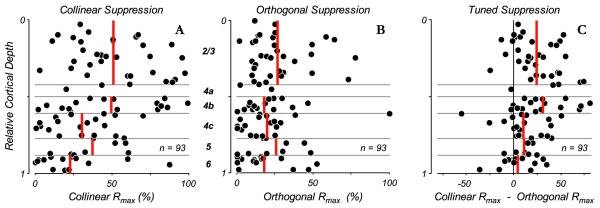
Suppression indices across cortical layers. Measures of maximum suppression strength (R_max parameter of fit to response suppression as a function of contrast) are plotted as a function of cortical layer for conditions in which stimuli of either collinear or orthogonal orientation were presented within the eCRF while the contrast in the CRF was the C₉₀ value for each neuron. R_max values of 0% indicate no modulation from eCRF stimulation and values near 100% indicate complete suppression of the neural response. Red vertical lines indicate mean values within each layer. A: the distribution of suppression strengths is shown for collinear stimuli in the eCRF. B: distribution of suppression strengths for an orthogonal orientation in the eCRF. The suppression strength across layers with orthogonal stimuli was reduced compared to collinear orientation in the eCRF, yet there were still some neurons that showed strong suppression. C: the suppression strength of the orientation-tuned component, i.e. the differences in suppression between (A) and (B), was greatest in layers 2/3 and 4b (24 ± 4% and 31 ± 7%, respectively) and much weaker in layers 5 (11 ± 4%) and 6 (5 ± 5%, mean ± s.e.m.).

To estimate how the orientation tuning of suppression varied across cortical layers we estimated tuned suppression as the difference in suppression strengths (difference between the R_max values) between collinear and orthogonal eCRF (Fig. 7C). Tuned suppression was strongly dominant in layers 2/3 and 4b (24 ± 4% and 31 ± 7% mean ± s.e.m., respectively), but was weaker in the input layer 4c (11 ± 6%) and in layer 5 (11 ± 4%). In layer 6 there was little eCRF suppression for either collinear or orthogonal stimuli. Consequently the suppression difference was almost zero (5 ± 5%). These measures of the strength of tuned suppression varied significantly across layers (p = 0.018, Kruskal-Wallis test). Thus, an orientation-tuned component of eCRF suppression (Levitt and Lund, 1997; Cavanaugh et al., 2002b) appears to be generated in specific local circuits within V1, and is manifested predominantly in the supragranular cortical layers 2/3 and 4b which also provide the major direct output from V1 to visual areas V2 and MT.

Temporal dynamics of eCRF modulation: tuned and untuned suppression

To tease apart the circuits underlying eCRF mechanisms, the temporal dynamics of modulation were analyzed. The preceding analyses in this paper focused on steady-state measures of CRF modulation from stimuli in the eCRF: responses averaged over the entire duration of the stimulus presentation. The dynamics of the development of different response components have been used to study cortical mechanisms of selectivity (Ringach et al., 1997; 2002; 2003; Xing et al., 2011). Response timing has also been used to infer intracortical processes involved directly in eCRF processing (Bair et al., 2003; Smith et al., 2006). Here we report on the temporal response properties of the suppression and their dependence on contrast and orientation of stimuli presented to the eCRF. Because the analysis was based on the timing of spike rate, the analysis was applied only to complex cells in the population of V1 cells studied. Since neurons can differ in their response latencies to the presentation of a stimulus, and to better compare temporal response dynamics across neurons, we aligned the responses to all stimulus conditions for each neuron to the time of its CRF response onset to an optimal grating.

We investigated how changes in the visual stimuli used here affected neurons’ temporal response profiles. We first measured changes in the timing of responses from the CRF with contrast. Because eCRF modulation is only detectable in the presence of CRF responses and is often measured relative in time to CRF responses, changes in CRF onset latency with contrast could influence the apparent arrival time of eCRF signals. Next, we show that the onset latency of eCRF suppression was also systematically influenced by eCRF stimulus contrast. Finally we demonstrate different response dynamics for the two components of eCRF suppression (orientation-untuned and -tuned). Tuned- and untuned-suppression from the eCRF were engaged across the entire contrast range. Together, these functional properties and their associated delays will combine to dynamically influence signaling of contextual modulation in V1.

Onset latencies with contrast

The initial goal was to measure the onset latency for CRF responses and eCRF suppression. First we measured response onset latency as a function of contrast for the optimal spatio-temporal stimulus confined to the classical receptive field. For individual complex cells onset latencies were estimated to be the first time point at which the stimulus-driven cumulative spike counts significantly exceeded the cumulative spike counts for spontaneous activity. Across the complex cell population onset latencies for stimuli of both C₉₀ and C₅₀ contrast (Fig. 8A) were significantly correlated (r=0.67, p < 0.0001) and lie below the unity line, indicating that response onset latencies were longer when the contrast of a stimulus in the CRF was lowered (Gawne et al., 1996; Carandini et al., 1997). On average, neurons’ response onset was delayed by 20ms when the contrast was lowered from that producing 90% of the maximal response to that eliciting half maximal response (Fig. 8B).

Fig. 8.

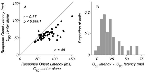
Change in CRF response onset latency with contrast. A: response onset latencies for stimuli driving the CRF alone are shown for C₅₀ and C₉₀ contrasts. The latency was determined to be the first time point where the stimulus-driven cumulative spike count was significantly greater than that of the spontaneous activity (see Methods). With lower contrast (C₅₀) the response onset latencies increase, as shown by the points lying below the unity line. B: histogram of the difference in onset latency between the C₅₀ and C₉₀ conditions. The average increase in latency due to lowering of stimulus contrast from C₉₀ to C₅₀ was 20 ms.

Given that the onset of neurons’ excitatory response was contrast-dependent, we further asked whether suppression from the eCRF also exhibited a temporal contrast-dependence. The onset of eCRF suppression, for CRF stimulation at C₉₀, was determined to be the first time at which the cumulative spike count was significantly lower than that of CRF stimulation alone (see Methods). Figures 9A-B show cumulative spike counts of two neurons to stimulation of their CRFs alone (red traces) as well as co-stimulation of their eCRFs (grey traces). Both neurons show that the time of suppression onset was shortest for the highest contrast stimuli (80%) in the eCRF. As the contrast of the eCRF stimulus was lowered, the time of suppression onset was delayed by tens of milliseconds for the neuron in Fig. 9A and by more than one hundred milliseconds for the neuron in Fig. 9B.

Fig. 9.

Change in eCRF suppression onset latency with stimulus suppression strength in the eCRF. A, B: cumulative spike counts are shown for two example neurons for optimal CRF stimuli at a contrast of C₉₀ within the CRF alone (no eCRF contrast: red traces) and with progressively higher contrasts of the collinear stimulus in the eCRF (10%, 20%, 80%: grey traces). The width of each trace indicates the mean ± 1 s.d. of the cumulative spike count over time. Both neurons showed the earliest suppression onset for eCRF stimuli of 80% contrast. As contrast was lowered, onset latencies for suppression increased by tens of milliseconds for the example cells shown on A, and sometimes by as much as one hundred milliseconds or more as for the cell shown in B. The three vertical lines in A and B show the latency for the onset of suppression for each of the three contrast levels, as estimated using a statistical criterion (see Methods). Small arrows indicate suppression onset latency determined by the time at which suppression reaches 5% of its cumulative effect over the 500 ms stimulus presentation. C: time of suppression onset latency (relative to response onset from the CRF) is plotted as a function of the suppression index (calculated over the entire stimulus presentation) for all eCRF conditions that produced at least 15% suppression of the neuronal response. While many stimuli suppressed the responses immediately around the time of CRF response onset (0 ms), suppression onset was often delayed by up to hundreds of milliseconds. Further, eCRF induced suppression onset latency was significantly negatively correlated with suppression strength (r=-0.24, p< 0.0001) indicating that weaker suppression tended to arrive later. D: smoothed plot of the data in (C) showing the median onset latency of suppression ± 1 s.e.m. (grey region) averaged using a boxcar of width 10%. While strong suppression arrived around the time of CRF response onset, weaker suppression tended to be delayed by around 40 ms. E: the onset latency of suppression increased as stimulus contrast within the eCRF was lowered.

Over all neurons, eCRF orientations, and contrasts, the eCRF onset latency (relative to excitatory CRF onset latency) was significantly negatively correlated with suppression strength (Fig. 9C; r=-0.24, p < 0.0001) indicating that weaker suppression tended to arrive later (as previously shown by Bair et al., 2003). For many conditions, suppression onset occurred close to the time of CRF onset (0 ms); however, it is also clear that the onset of suppression can also be delayed by more than one hundred milliseconds. The median eCRF suppression onset latency (± 1 s.e.m.) in relation to suppression strength (averaged using a boxcar of 10% SI width) showed that across neurons strong suppression (SI>80%) arrived a few milliseconds after CRF onset, but weaker suppression (SI=20%) tended to be delayed by around 40 milliseconds on average (Fig. 9D). Measurement of the onset of suppression based upon a statistical criterion is indicative of the time at which eCRF modulation can influence downstream computation. The determination of when suppressive signals arrive within the recorded neuron may be influenced by the use of a statistical criterion: weak signals may appear to show delayed arrival due to the fact that they take longer to cross a statistical threshold. To address this, we estimated the onset of eCRF suppression using an alternate method (the first time point at which the eCRF produced 5% of the total suppression observed over the entire stimulus presentation, see arrows in Fig. 9A-B). This approach yielded shorter onset latencies for weaker suppression, nonetheless the overall results were similar with both methods, with relative suppression onset latency significantly negatively correlated with suppression strength (r=-0.21, p < 0.0001) and weak suppression showing longer relative onset latencies (34.8 ± 4.0 ms, median ± 1 s.e.m.). Analysis of suppression onset latency with regard to stimulus contrast in the eCRF revealed that on average across the population, suppression onset was systematically delayed as the contrast driving the eCRF was lowered (Fig. 9E). The timing of suppression onset relative to the onset of excitatory responses from the CRF is not simply a fixed feature of eCRF modulation, but is determined by contrast-dependent temporal integration within the eCRF, similar to effects observed in cortical neurons’ classical receptive fields (Gawne et al., 1996). These results have important implications for interpreting earlier studies where there were conflicting results on the timing of eCRF suppression (Bair et al., 2003; Muller et al., 2003; Smith et al., 2006) and hence where and how within the circuit the eCRF effects are generated. We elaborate further upon this matter in the Discussion.

Component mechanisms of eCRF suppression

In the first results section we reported that there was a difference in steady-state suppression strength with orientation (Fig. 5). To tease apart the components of eCRF suppression we examined how the timing of modulation depended upon the orientation of stimuli presented within the eCRF. The time course of response modulation by collinear and orthogonal stimuli in the eCRF enabled us to estimate the dynamics of tuned and untuned suppression coming from the eCRF. To obtain a population estimate of the effects of different eCRF stimulus conditions, the responses of each complex cell were aligned in time to the onset of the response to the stimulus in the CRF alone, normalized to the peak instantaneous firing rate to that stimulus, and then the responses for all cells were averaged for each eCRF stimulus contrast and orientation combination (Fig. 10, lines: mean values, shaded regions: ±1 s.e.m.).

Fig. 10.

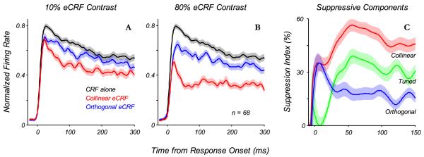
Temporal dynamics of eCRF suppression. The average response dynamics to a stimulus in the CRF, with the preferred stimulus parameters and a C₉₀ contrast, when different stimuli are presented to the eCRF. All responses were first normalized to the peak response to the stimulus in the CRF alone (no eCRF modulation), and taken from the time of response onset to the stimulus in the CRF alone. A: response dynamics to a stimulus in the CRF with no eCRF stimulus (black) as well as with collinear (red) and orthogonal (blue) stimuli in the eCRF presented at 10% contrast (lines: mean values, shaded regions: ±1 s.e.m.). At the earliest times there was very little suppression from the eCRF stimuli, whereas later in time (30-40 ms) there developed a stronger suppression from the collinear eCRF stimulus. B: similar plots to (A), except here, stimuli in the eCRF were presented at 80% contrast. At earliest times (0-25 ms) there was some suppression from both eCRF stimuli, with stronger suppression coming from the collinear eCRF stimulus later (25-50 ms). C: to better highlight the dynamics, responses from (B) are re-plotted here as the percentage of response suppression. The suppressive components coming from the collinear and orthogonal eCRF stimuli are shown in red and blue, respectively. Plotted in green is the difference between those two curves, what we term the tuned suppressive component, which did not begin to develop until 25-50 ms.

The first significant result was that the initial suppression was independent of stimulus orientation in the eCRF (Fig. 10A, 10% eCRF contrast, compare red and blue curves). However, at later points in time the collinear stimulus in the eCRF exerted stronger suppression than the orthogonal stimulus. At higher eCRF contrasts (Fig. 10B, 80% contrast) a similar pattern held, with the exception that overall eCRF suppression was stronger and arrived earlier. The difference in the strength of suppression between the collinear and orthogonal eCRF conditions showed the time course of the orientation-tuned component of suppression (Fig, 10C, green curve). Based on the average responses, the tuned component of suppression was about 20-30 ms delayed relative to the early, untuned component that was similar for both the collinear and the orthogonal eCRF stimulus. We term this early component untuned suppression, the component of suppression from the orthogonal stimulus in the eCRF, and suggest that it shows the same latency and amplitude whether elicited by the collinear or orthogonal stimulus, or any orientations in between. The tuned component of suppression reached its peak at about 50-60 ms after the CRF response onset.

It is important to determine how the tuned and untuned components of suppression developed in time with contrast. In the early period (1-25 ms) after response onset, the strengths of suppression for collinear and orthogonal stimuli at the highest contrast tested (80%) were relatively similar (Fig. 11A). In later periods there was a shift in relative strength so that by 50 ms the main component of suppression was associated with the collinear stimulus (Fig. 11B-D). It should be noted that for a very small number of neurons there was some facilitation evident in the selected integration windows, as indicated by suppression indices with negative values. The relationship between the dynamics of eCRF facilitation and suppression will be addressed more thoroughly in a companion study.

Fig. 11.

Comparison of suppression to collinear and orthogonal stimuli over time. Suppression indices for 68 complex cells for collinear and orthogonal eCRF stimuli at 80% contrast were calculated as a function of time in 25 ms bins, where t is time from CRF response onset, and 100% represents complete suppression of the response and 0% represents no suppression, negative SI values indicate response facilitation. A: at the earliest times (1-25 ms) the amount of suppression was approximately equal between the two conditions, as shown by points lying along the unity line. The point in red indicates the mean suppression over all neurons. B: at later times (26-50 ms), stronger suppression from the collinear eCRF stimulus started to become evident, which persisted at later time points (C, D). E: the average suppression indices are plotted for the population of cells to illustrate how suppression developed across time and across contrasts. The size of the dot indicates the contrast presented in the eCRF, with larger sizes indicating higher contrasts. The color of the dot indicates the time bin over which the suppression indices were measured. At earliest times (black) the suppression between the two stimuli was equal, with higher contrasts inducing greater suppression. At later time points (red, blue, green), for all contrasts, suppression from the collinear stimuli in the eCRF was greater than from orthogonal stimuli.

To determine the effect of contrast in the eCRF on the time course of the differential development of collinear and orthogonal suppression, we calculated the average suppression, across the 68 neurons tested, for each time interval at each contrast. Time dependent changes in the ratio of collinear to orthogonal suppression were evident at all stimulus contrasts. In this summary plot (Fig. 11E), the size of the dot indicates eCRF stimulus contrast and the color indicates successive time windows (black, red, blue, and green, respectively). For high contrast stimuli (80% contrast, large dots) the collinear and orthogonal suppression are approximately equal in the 1-25 ms integration window, but collinear suppression strengthens and orthogonal suppression weakens at later time points (data re-plotted from mean values in Fig. 11A-D). The same temporal sequences can be traced for lower contrasts.

Note that in both Figs. 10C and 11E, the time course of untuned suppression (i.e. equal strength across eCRF orientations) is not only more rapidly-rising than that of tuned suppression, but it also is more transient in time, with a decay in strength from 1-25 ms to 76-100 ms. The different time waveforms of the tuned and untuned eCRF responses support the idea that tuned and untuned suppression are two distinct mechanisms that contribute to eCRF suppression. The importance of the dynamical properties on understanding of the cortical circuits involved in eCRF modulation are presented in more detail in the Discussion.

DISCUSSION

Objects and contours in natural images are often spatially extended beyond a neuron’s CRF and scenes contain low or intermediate contrast energy (Tadmor & Tolhurst, 2000). We report robust suppressive eCRF mechanisms in V1 that are engaged at low contrasts and across a wide contrast range. While we did not find strong eCRF facilitation, other studies (Ichida et al., 2007) have shown that facilitation is mainly observed either when stimuli are absent from the region abutting the CRF or when the CRF is weakly or suboptimally stimulated (Polat et al., 1998; Ichida et al., 2007; Shushruth et al., 2012). Given the spatially extended contours present in natural scenes and the suppression we observe from large stimuli across a range of stimulus contrasts, we think that eCRF mechanisms we describe in this study are likely to generalize to cortical network engagement under behaviorally-relevant conditions.

Contrast sensitivity and eCRF circuits

Of the 114 neurons studied, 88% showed greater than 15% response suppression from at least one of the stimuli presented to the eCRF. For both collinear and orthogonal eCRF stimuli, the contrast that evoked half maximal eCRF suppression was often lower than for CRF excitation (Fig. 4C-D). A similar result for collinear stimuli was reported for cat area 17 (Sadakane et al., 2006). For collinear eCRF stimuli, a substantial fraction of our population (~50%) had C₅₀’s below 10% contrast (Fig. 4A) and thus displayed suppression at very low contrasts.

Strong low-contrast suppression suggests a suppressive contribution from cortical neurons in the magnocellular pathway. This pathway has been associated with low contrast thresholds (Kaplan & Shapley, 1986; Hawken et al., 1988) and responds best to achromatic stimuli (Wiesel and Hubel, 1966). In V1, eCRF suppression is reported to be predominantly achromatic (Solomon et al., 2004). The possibility that magnocellular-driven signals contribute to the eCRF is of particular interest in superficial layers (layer 2/3) of V1, where the CRF C₅₀ is relatively high and characteristic of parvocellular pathway input but the eCRF C₅₀ is low and indicative of the magnocellular pathway (Fig. 6D). This result suggests that local circuit models of CRF-eCRF suppressive mechanisms (Cavanaugh et al., 2002a; Ayaz & Chance, 2009; Ozeki et al., 2009; Schwabe et al., 2010) should incorporate functional inputs with parvocellular-like signals to the CRF and magnocellular-like signals to the eCRF for the majority of layer 2/3 neurons.

Orientation selectivity and eCRF circuits

Based on their tuning profiles, the orientation-selective components of suppression (Levitt & Lund, 1997; Cavanaugh et al., 2002b; Xing et al., 2005; Webb et al., 2005) are of presumed cortical origin. Earlier studies on V1 neurons’ size-tuning reported that the strongest eCRF suppression was in layers 2/3 and 4b (Sceniak et al., 2001; Shushruth et al., 2009; Shushruth et al., 2013). Strong size-tuning could be due either to orientation-independent or orientation-dependent suppression. Our current study showed that superficial-layer neurons, which have the strongest eCRF suppression, also exhibited the strongest orientation-tuned eCRF suppression (Fig. 7C). Neurons in input (4c) and deep layers (5 and 6) showed much weaker tuned suppression, accounting for their weaker eCRF suppression overall. However, recently Shushruth et al. (2013) reported that neurons in layer 4cα also showed strong tuned suppression while the suppression in 4cβ was somewhat weaker and less tuned. They found that this difference in tuning was most evident from stimulation of the near surround, which is the eCRF region our stimuli are likely to have most strongly engaged. The differences in strength and tuning of eCRF modulation in 4cα and 4cβ between the two studies needs to be resolved but may be partially due to the relatively small sample sizes from these sublaminae. In our study, we find that the tuning selectivity of the eCRF was preserved across a wide contrast range (Fig. 10, 11E). In summary, tuned eCRF suppression appeared to be generated and amplified within the cortical layers that provide the principal output to extrastriate cortex but it was largely absent from the input layers and infragranular layers of V1. Previously, in studying the dynamics of orientation selectivity Xing et al. (2005) found a significant component of tuned suppression from within and near the CRF in all cortical layers. The current study focused upon the responses from stimuli confined to the eCRF. Reconciling the results in infragranular layers will require investigation into the precise spatial extent of these suppressive mechanisms.

The origin of eCRF untuned suppression is a matter of debate. Based upon spatial tuning characteristics (broad orientation and spatio-temporal frequency tuning), Webb et al. (2005) suggested that this eCRF component was likely inherited from the LGN, as also suggested by Sadakane et al. (2006). While LGN neurons exhibit eCRF suppression, particularly magnocellular cells in macaque (Sceniak et al. 2006; Alitto et al. 2008) and marmoset (Solomon et al., 2002), these neurons are likely to be maximally suppressed by stimuli at optimal sizes for V1 CRFs (as previously pointed out by Ozeki et al., 2004). Another potential explanation of untuned suppression is that a population of broadly tuned cortical neurons provides eCRF input. V1 has a pool of neurons that are broadly orientation- and spatial-frequency-tuned (Ringach et al., 2002; Xing et al., 2004) that could form the neural substrate for untuned suppression. If the untuned suppression from the eCRF is cortical in origin it still needs to be determined whether it is an extension of the same untuned suppression (Xing et al, 2005) or normalization signal (Smith et al, 2006) that is underlying the CRF or it is a separate mechanism.

Response dynamics of eCRF suppression

Numerous psychophysical and neurophysiological studies have varied the spatial separation between central and flanking stimuli to determine whether changes in the onset latency of modulation are consistent with the conduction velocities of long-range horizontal axons in V1. While one study of V1 physiology (Bair et al., 2003) found delays to be inconsistent with a horizontal propagation explanation other psychophysical studies (Cass and Spehar 2005) argued that eCRF modulation was consistent with horizontal propagation. We showed that stimuli with constant spatial structure exhibited relative increases in eCRF onset latency due to a reduction of stimulus contrast or drive, which is in agreement with the contrast-dependent integration properties of cortical neurons (Gawne et al., 1996). On average, a reduction of eCRF stimulus contrast led to a ~40ms increase in suppression onset. This delay, if interpreted as coming from V1 horizontal connections with conduction velocities of 0.1m/s, implies signals propagating from 4mm lateral in cortex which is the anatomical extent of horizontal connections. Thus, we caution that contrast-integration delays present a confound to attempts to use the time of modulation onset to link eCRF signals to precise horizontal circuitry in V1 cortex.

Across a wide contrast range, we found two eCRF suppressive components with distinct orientation tuning profiles: a shorter latency untuned component and a longer latency tuned component that often had a larger response magnitude (Fig. 10). The temporal dynamics of the tuning of eCRF modulation explain a number of conflicting results from earlier studies. Muller et al. (2003) reported that suppression was coincident or earlier in time than CRF response onset whereas Bair et al. (2003) showed that eCRF suppression was often relatively delayed by 10-30 ms. When comparing the CRF response onset with the response to the same stimulus with a high-contrast collinear stimulus in the eCRF, suppression can occur as early as CRF onset (Muller et al., 2003) a result we confirmed (Fig. 9C). However, this early suppression was not orientation-tuned (Fig. 10C, 11E). Conversely, measuring the difference in response profile between two eCRF conditions with different stimulus orientations, as done in Bair et al. (2003) and Smith et al. (2006), is akin to measuring the tuned component of eCRF suppression which arrives with longer latency. Studies of figure-ground segregation have also used this latter comparison method (Lamme, 1995; Super et al., 2001) in which an oriented object covering the CRF is made more or less salient by an orthogonal or collinear background, respectively. Neural activity was reduced for the collinear condition. The difference-signal onset appeared at moderate latency and was reported to be observed only in the cortex of the awake, behaving primate, leading to the conclusion that it was a higher-level, behavioral figure-ground signal. Our results on the sufentanyl-anesthetized preparation suggest an alternative interpretation of the figure-ground results of Lamme et al., namely that such results are consistent with the delayed emergence of the orientation-tuned component of eCRF suppression we measured.

Summary

In summary, the current study showed a clear elaboration of contextual effects from the input (layer 4c) to the cortico-cortical output layers (layers 2/3 and 4b), where orientation-tuned eCRF suppression was predominant and the contrast that first evoked suppression was relatively low. This high contrast sensitivity is a signature of the achromatic magnocellular pathway and suggests that the eCRF in many neurons, whether their CRF is dominated by magnocellular or parvocellular signals, will be activated by low to intermediate contrast stimuli in natural scenes (Tadmor & Tolhurst, 2000). In addition we showed that changes in stimulus contrast and orientation systematically influence the temporal evolution of eCRF modulation. Perceptually, the dynamic changes in eCRF properties are likely to be relevant under natural viewing where fixation durations can last a few hundred milliseconds due to saccadic eye movements. Perceptual contextual modulation will be affected by both stimulus properties and viewing duration. For many aspects of visual object recognition, such as figure-ground segregation (Super et al., 2010), border-ownership coding (Zhang and von der Heydt, 2010), and natural viewing (Vinje and Gallant, 2002), the response properties of V1 neurons’ eCRFs are likely to be influential in the computations required for perception.

REFERENCES

- Alitto HJ, Usrey WM. Origin and dynamics of extraclassical suppression in the lateral geniculate nucleus of the macaque monkey. Neuron. 2008;57:135–146. doi: 10.1016/j.neuron.2007.11.019. [DOI] [PMC free article] [PubMed] [Google Scholar]
- Allman J, Miezin F, McGuinness E. Stimulus specific responses from beyond the classical receptive field: neurophysiological mechanisms for local-global comparisons in visual neurons. Annu Rev Neurosci. 1985;8:407–430. doi: 10.1146/annurev.ne.08.030185.002203. [DOI] [PubMed] [Google Scholar]
- Ayaz A, Chance FS. Gain modulation of neuronal responses by subtractive and divisive mechanisms of inhibition. J Neurophysiol. 2009;101:958–968. doi: 10.1152/jn.90547.2008. [DOI] [PubMed] [Google Scholar]
- Bair W, Cavanaugh JR, Movshon JA. Time course and time-distance relationships for surround suppression in macaque V1 neurons. J Neurosci. 2003;23:7690–7701. doi: 10.1523/JNEUROSCI.23-20-07690.2003. [DOI] [PMC free article] [PubMed] [Google Scholar]
- Baker DH, Graf EW. Contextual effects in speed perception may occur at an early stage of processing. Vision Res. 2010;50:193–201. doi: 10.1016/j.visres.2009.11.011. [DOI] [PubMed] [Google Scholar]
- Blakemore C, Tobin EA. Lateral inhibition between orientation detectors in the cat’s visual cortex. Exp Brain Res. 1972;15:439–440. doi: 10.1007/BF00234129. [DOI] [PubMed] [Google Scholar]
- Bonds AB. Temporal dynamics of contrast gain in single cells of the cat striate cortex. Vis Neurosci. 1991;6:239–255. doi: 10.1017/s0952523800006258. [DOI] [PubMed] [Google Scholar]
- Carandini M, Heeger DJ, Movshon JA. Linearity and normalization in simple cells of the macaque primary visual cortex. J Neurosci. 1997;17:8621–8644. doi: 10.1523/JNEUROSCI.17-21-08621.1997. [DOI] [PMC free article] [PubMed] [Google Scholar]
- Cass JR, Spehar B. Dynamics of collinear contrast facilitation are consistent with long-range horizontal striate transmission. Vision Res. 2005;45:2728–2739. doi: 10.1016/j.visres.2005.03.010. [DOI] [PubMed] [Google Scholar]
- Cavanaugh JR, Bair W, Movshon JA. Nature and interaction of signals from the receptive field center and surround in macaque V1 neurons. J Neurophysiol. 2002a;88:2530–2546. doi: 10.1152/jn.00692.2001. [DOI] [PubMed] [Google Scholar]
- Cavanaugh JR, Bair W, Movshon JA. Selectivity and spatial distribution of signals from the receptive field surround in macaque V1 neurons. J Neurophysiol. 2002b;88:2547–2556. doi: 10.1152/jn.00693.2001. [DOI] [PubMed] [Google Scholar]
- Clatworthy PL, Chirimuuta M, Lauritzen JS, Tolhurst DJ. Coding of the contrasts in natural images by populations of neurons in primary visual cortex (V1) Vision Res. 2003;43:1983–2001. doi: 10.1016/s0042-6989(03)00277-3. [DOI] [PubMed] [Google Scholar]
- DeAngelis GC, Freeman RD, Ohzawa I. Length and width tuning of neurons in the cat’s primary visual cortex. J Neurophysiol. 1994;71:347–374. doi: 10.1152/jn.1994.71.1.347. [DOI] [PubMed] [Google Scholar]
- Gawne TJ, Kjaer TW, Richmond BJ. Latency: another potential code for feature binding in striate cortex. J Neurophysiol. 1996;76:1356–1360. doi: 10.1152/jn.1996.76.2.1356. [DOI] [PubMed] [Google Scholar]
- Gilbert CD. Laminar differences in receptive field properties of cells in cat primary visual cortex. J Physiol. 1977;268:391–421. doi: 10.1113/jphysiol.1977.sp011863. [DOI] [PMC free article] [PubMed] [Google Scholar]
- Hawken MJ, Parker AJ, Lund JS. Laminar organization and contrast sensitivity of direction-selective cells in the striate cortex of the Old World monkey. J Neurosci. 1988;8:3541–3548. doi: 10.1523/JNEUROSCI.08-10-03541.1988. [DOI] [PMC free article] [PubMed] [Google Scholar]
- Hawken MJ, Shapley RM, Grosof DH. Temporal-frequency selectivity in monkey visual cortex. Vis Neurosci. 1996;13:477–492. doi: 10.1017/s0952523800008154. [DOI] [PubMed] [Google Scholar]
- Ichida JM, Schwabe L, Bressloff PC, Angelucci A. Response facilitation from the “suppressive” receptive field surround of macaque V1 neurons. J Neurophysiol. 2007;98:2168–2181. doi: 10.1152/jn.00298.2007. [DOI] [PubMed] [Google Scholar]
- Kapadia MK, Westheimer G, Gilbert CD. Dynamics of spatial summation in primary visual cortex of alert monkeys. Proc Natl Acad Sci U S A. 1999;96:12073–12078. doi: 10.1073/pnas.96.21.12073. [DOI] [PMC free article] [PubMed] [Google Scholar]
- Kapadia MK, Westheimer G, Gilbert CD. Spatial distribution of contextual interactions in primary visual cortex and in visual perception. J Neurophysiol. 2000;84:2048–2062. doi: 10.1152/jn.2000.84.4.2048. [DOI] [PubMed] [Google Scholar]
- Kaplan E, Shapley RM. The primate retina contains two types of ganglion cells, with high and low contrast sensitivity. Proc Natl Acad Sci U S A. 1986;83:2755–2757. doi: 10.1073/pnas.83.8.2755. [DOI] [PMC free article] [PubMed] [Google Scholar]
- Lamme VA. The neurophysiology of figure-ground segregation in primary visual cortex. J Neurosci. 1995;15:1605–1615. doi: 10.1523/JNEUROSCI.15-02-01605.1995. [DOI] [PMC free article] [PubMed] [Google Scholar]
- Levitt JB, Lund JS. Contrast dependence of contextual effects in primate visual cortex. Nature. 1997;387:73–76. doi: 10.1038/387073a0. [DOI] [PubMed] [Google Scholar]
- Levitt JB, Lund JS. The spatial extent over which neurons in macaque striate cortex pool visual signals. Vis Neurosci. 2002;19:439–452. doi: 10.1017/s0952523802194065. [DOI] [PubMed] [Google Scholar]
- Li W, Piech V, Gilbert CD. Contour saliency in primary visual cortex. Neuron. 2006;50:951–962. doi: 10.1016/j.neuron.2006.04.035. [DOI] [PubMed] [Google Scholar]
- Merrill EG, Ainsworth A. Glass-coated platinum-plated tungsten microelectrodes. Med Biol Eng. 1972;10:662–672. doi: 10.1007/BF02476084. [DOI] [PubMed] [Google Scholar]
- Muller JR, Metha AB, Krauskopf J, Lennie P. Local signals from beyond the receptive fields of striate cortical neurons. J Neurophysiol. 2003;90:822–831. doi: 10.1152/jn.00005.2003. [DOI] [PubMed] [Google Scholar]
- Naka KI, Rushton WA. S-potentials from luminosity units in the retina of fish (Cyprinidae) J Physiol. 1966;185:587–599. doi: 10.1113/jphysiol.1966.sp008003. [DOI] [PMC free article] [PubMed] [Google Scholar]
- Ozeki H, Sadakane O, Akasaki T, Naito T, Shimegi S, Sato H. Relationship between excitation and inhibition underlying size tuning and contextual response modulation in the cat primary visual cortex. J Neurosci. 2004;24:1428–1438. doi: 10.1523/JNEUROSCI.3852-03.2004. [DOI] [PMC free article] [PubMed] [Google Scholar]
- Ozeki H, Finn IM, Schaffer ES, Miller KD, Ferster D. Inhibitory stabilization of the cortical network underlies visual surround suppression. Neuron. 2009;62:578–592. doi: 10.1016/j.neuron.2009.03.028. [DOI] [PMC free article] [PubMed] [Google Scholar]
- Polat U, Mizobe K, Pettet MW, Kasamatsu T, Norcia AM. Collinear stimuli regulate visual responses depending on cell’s contrast threshold. Nature. 1998;391:580–584. doi: 10.1038/35372. [DOI] [PubMed] [Google Scholar]
- Ringach DL, Hawken MJ, Shapley R. Dynamics of orientation tuning in macaque primary visual cortex. Nature. 1997;387:281–284. doi: 10.1038/387281a0. [DOI] [PubMed] [Google Scholar]
- Ringach DL, Shapley RM, Hawken MJ. Orientation selectivity in macaque V1: diversity and laminar dependence. J Neurosci. 2002;22:5639–5651. doi: 10.1523/JNEUROSCI.22-13-05639.2002. [DOI] [PMC free article] [PubMed] [Google Scholar]
- Ringach DL, Hawken MJ, Shapley R. Dynamics of orientation tuning in macaque V1: the role of global and tuned suppression. J Neurophysiol. 2003;90:342–352. doi: 10.1152/jn.01018.2002. [DOI] [PubMed] [Google Scholar]
- Sadakane O, Ozeki H, Naito T, Akasaki T, Kasamatsu T, Sato H. Contrast-dependent, contextual response modulation in primary visual cortex and lateral geniculate nucleus of the cat. Eur J Neurosci. 2006;23:1633–1642. doi: 10.1111/j.1460-9568.2006.04681.x. [DOI] [PubMed] [Google Scholar]
- Sceniak MP, Ringach DL, Hawken MJ, Shapley R. Contrast’s effect on spatial summation by macaque V1 neurons. Nat Neurosci. 1999;2:733–739. doi: 10.1038/11197. [DOI] [PubMed] [Google Scholar]
- Sceniak MP, Hawken MJ, Shapley R. Visual spatial characterization of macaque V1 neurons. J Neurophysiol. 2001;85:1873–1887. doi: 10.1152/jn.2001.85.5.1873. [DOI] [PubMed] [Google Scholar]
- Sceniak MP, Chatterjee S, Callaway EM. Visual spatial summation in macaque geniculocortical afferents. J Neurophysiol. 2006;96:3474–3484. doi: 10.1152/jn.00734.2006. [DOI] [PubMed] [Google Scholar]
- Schwabe L, Obermayer K, Angelucci A, Bressloff PC. The role of feedback in shaping the extra-classical receptive field of cortical neurons: a recurrent network model. J Neurosci. 2006;26:9117–9129. doi: 10.1523/JNEUROSCI.1253-06.2006. [DOI] [PMC free article] [PubMed] [Google Scholar]
- Schwabe L, Ichida JM, Shushruth S, Mangapathy P, Angelucci A. Contrast-dependence of surround suppression in Macaque V1: experimental testing of a recurrent network model. Neuroimage. 2010;52:777–792. doi: 10.1016/j.neuroimage.2010.01.032. [DOI] [PMC free article] [PubMed] [Google Scholar]
- Sengpiel F, Sen A, Blakemore C. Characteristics of surround inhibition in cat area 17. Exp Brain Res. 1997;116:216–228. doi: 10.1007/pl00005751. [DOI] [PubMed] [Google Scholar]
- Shushruth S, Ichida JM, Levitt JB, Angelucci A. Comparison of spatial summation properties of neurons in macaque V1 and V2. J Neurophysiol. 2009;102:2069–2083. doi: 10.1152/jn.00512.2009. [DOI] [PMC free article] [PubMed] [Google Scholar]
- Shushruth S, Mangapathy P, Ichida JM, Bressloff PC, Schwabe L, Angelucci A. Strong recurrent networks compute the orientation tuning of surround modulation in the primate primary visual cortex. J Neurosci. 2012;32:308–321. doi: 10.1523/JNEUROSCI.3789-11.2012. [DOI] [PMC free article] [PubMed] [Google Scholar]
- Shushruth S, Nurminen L, Bijanzadeh M, Ichida JM, Vanni S, Angelucci A. Different orientation tuning of near- and far-surround suppression in macaque primary visual cortex mirrors their tuning in human perception. J Neurosci. 2013;33:106–119. doi: 10.1523/JNEUROSCI.2518-12.2013. [DOI] [PMC free article] [PubMed] [Google Scholar]
- Sillito AM, Grieve KL, Jones HE, Cudeiro J, Davis J. Visual cortical mechanisms detecting focal orientation discontinuities. Nature. 1995;378:492–496. doi: 10.1038/378492a0. [DOI] [PubMed] [Google Scholar]
- Smith MA, Bair W, Movshon JA. Dynamics of suppression in macaque primary visual cortex. J Neurosci. 2006;26:4826–4834. doi: 10.1523/JNEUROSCI.5542-06.2006. [DOI] [PMC free article] [PubMed] [Google Scholar]
- Solomon SG, White AJ, Martin PR. Extraclassical receptive field properties of parvocellular, magnocellular, and koniocellular cells in the primate lateral geniculate nucleus. J Neurosci. 2002;22:338–349. doi: 10.1523/JNEUROSCI.22-01-00338.2002. [DOI] [PMC free article] [PubMed] [Google Scholar]
- Solomon SG, Peirce JW, Lennie P. The impact of suppressive surrounds on chromatic properties of cortical neurons. J Neurosci. 2004;24:148–160. doi: 10.1523/JNEUROSCI.3036-03.2004. [DOI] [PMC free article] [PubMed] [Google Scholar]
- Somers DC, Todorov EV, Siapas AG, Toth LJ, Kim DS, Sur M. A local circuit approach to understanding integration of long-range inputs in primary visual cortex. Cereb Cortex. 1998;8:204–217. doi: 10.1093/cercor/8.3.204. [DOI] [PubMed] [Google Scholar]
- Super H, Spekreijse H, Lamme VA. Two distinct modes of sensory processing observed in monkey primary visual cortex (V1) Nat Neurosci. 2001;4:304–310. doi: 10.1038/85170. [DOI] [PubMed] [Google Scholar]
- Super H, Romeo A, Keil M. Feed-forward segmentation of figure-ground and assignment of border-ownership. PLoS One. 2010;5:e10705. doi: 10.1371/journal.pone.0010705. [DOI] [PMC free article] [PubMed] [Google Scholar]
- Tadmor Y, Tolhurst DJ. Calculating the contrasts that retinal ganglion cells and LGN neurones encounter in natural scenes. Vision Res. 2000;40:3145–3157. doi: 10.1016/s0042-6989(00)00166-8. [DOI] [PubMed] [Google Scholar]
- Vinje WE, Gallant JL. Natural stimulation of the nonclassical receptive field increases information transmission efficiency in V1. J Neurosci. 2002;22:2904–2915. doi: 10.1523/JNEUROSCI.22-07-02904.2002. [DOI] [PMC free article] [PubMed] [Google Scholar]
- Webb BS, Dhruv NT, Solomon SG, Tailby C, Lennie P. Early and late mechanisms of surround suppression in striate cortex of macaque. J Neurosci. 2005;25:11666–11675. doi: 10.1523/JNEUROSCI.3414-05.2005. [DOI] [PMC free article] [PubMed] [Google Scholar]
- Wiesel TN, Hubel DH. Spatial and chromatic interactions in the lateral geniculate body of the rhesus monkey. J Neurophysiol. 1966;29:1115–1156. doi: 10.1152/jn.1966.29.6.1115. [DOI] [PubMed] [Google Scholar]
- Xing D, Ringach DL, Shapley R, Hawken MJ. Correlation of local and global orientation and spatial frequency tuning in macaque V1. J Physiol. 2004;557:923–933. doi: 10.1113/jphysiol.2004.062026. [DOI] [PMC free article] [PubMed] [Google Scholar]
- Xing D, Shapley RM, Hawken MJ, Ringach DL. Effect of stimulus size on the dynamics of orientation selectivity in macaque V1. J Neurophysiol. 2005;94:799–812. doi: 10.1152/jn.01139.2004. [DOI] [PubMed] [Google Scholar]
- Xing D, Ringach DL, Hawken MJ, Shapley RM. Untuned suppression makes a major contribution to the enhancement of orientation selectivity in macaque V1. J Neurosci. 2011;31:15972–15982. doi: 10.1523/JNEUROSCI.2245-11.2011. [DOI] [PMC free article] [PubMed] [Google Scholar]
- Yazdanbakhsh A, Livingstone MS. End stopping in V1 is sensitive to contrast. Nat Neurosci. 2006;9:697–702. doi: 10.1038/nn1693. [DOI] [PMC free article] [PubMed] [Google Scholar]
- Zhang NR, von der Heydt R. Analysis of the context integration mechanisms underlying figure-ground organization in the visual cortex. J Neurosci. 2010;30:6482–6496. doi: 10.1523/JNEUROSCI.5168-09.2010. [DOI] [PMC free article] [PubMed] [Google Scholar]