Diversity of neural responses in the brainstem during smooth pursuit eye movements constrains the circuit mechanisms of neural integration

Abstract

Neural integration converts transient events into sustained neural activity. In the smooth pursuit eye movement system, neural integration is required to convert cerebellar output into the sustained discharge of extraocular motoneurons. We recorded the expression of integration in the time-varying firing rates of cerebellar and brainstem neurons in the monkey during pursuit of step-ramp target motion. Electrical stimulation with single shocks in the cerebellum identified brainstem neurons that are monosynaptic targets of inhibition from the cerebellar floccular complex. They discharge in relation to eye acceleration, eye velocity, and eye position, with a stronger acceleration signal than found in most other brainstem neurons. The acceleration and velocity signals can be accounted for by opponent contributions from the two sides of the cerebellum, without integration; the position signal implies participation in the integrator. Other neurons in the vestibular nucleus show a wide range of blends of signals related to eye velocity and eye position, reflecting different stages of integration. Neurons in the Abducens nucleus discharge homogeneously in relation mainly to eye position, and reflect almost perfect integration of the cerebellar outputs. Average responses of neural populations and the diverse individual responses of large samples of individual neurons are reproduced by a hierarchical neural circuit based on a model suggested the anatomy and physiology of the larval zebrafish brainstem. The model uses a combination of feed-forward and feedback connections to support a neural circuit basis for integration in monkeys and other species.

Introduction

Neural integration converts a transient event into a sustained response. In addition to its functions in oculomotor control (Skavenski and Robinson, 1973; Galiana and Outerbridge, 1984; Cannon and Robinson, 1985; Seung, 1996), integration maintains the memory of a sensory event long after the physical stimulus has vanished (Romo et al., 1999) and is a key factor in the accumulation of evidence for rendering complex perceptual decisions (Mazurek et al., 2003). An understanding of the neural mechanisms of integration in the brainstem oculomotor system may lead to understanding of the implementation of an essential neural computation that is used in many brain circuits, for multiple purposes.

We can understand the function of a neural circuit by studying the relation between its inputs and outputs. To understand how a circuit works, however, we must investigate the intermediate processing within the circuit. In smooth pursuit eye movements, we already have some knowledge of the time-varying firing rates of Purkinje cells in the cerebellum that provide the inputs to a brainstem circuit (Stone and Lisberger, 1990), and we can predict the time-varying output of that circuit in the discharge of extraocular motoneurons. Knowledge of these inputs and outputs reveals that integration in the mathematical sense is the function of the brainstem circuit (Shidara et al., 1993; Krauzlis and Lisberger, 1994). A number of prior papers have proposed neural circuit mechanisms for integration (Cannon et al., 1983; Galiana and Outerbridge, 1984; Cannon and Robinson, 1985; Seung, 1996; Miri et al., 2011), most based on recurrent connections within an integrating circuit. Missing, however, is an understanding of the pattern of recurrent connections that would allow the circuit to perform integration and would mimic the responses of real brainstem neurons during eye movement behavior.

Our goal was to move beyond the previous understanding of how the integrator circuit works through two approaches. First, by using electrical stimulation in the cerebellum to identify brainstem neurons that are on the input side of the integrator circuit, we can start to correlate different degrees of integration with the relative position of neurons within an integrator circuit. Second, by treating the diversity of the time-varying firing rates in the brainstem during the same, stereotyped smooth pursuit eye movement as meaningful, rather than simply as noisy variation, we can ask about the internal workings of the integrator circuit. Thus, we can address the key questions of whether substantial amount of integration is performed at the cerebellum target neurons, and whether the diversity of time-varying firing rates across the non-target neurons might arise within an integrator circuit (Miri et al., 2011). Our data suggest that integration occurs progressively in brainstem neurons, and that the diversity of time-varying neural responses is a natural consequence of a specific architecture in the connections of integrator circuits.

Our computational analysis takes off from a suggestion of Miri et al. (2011), who provided a major advance toward understanding the neural mechanisms of integration. Through calcium imaging during fixation eye movements in larval zebrafish, they suggested an integrating circuit in which the connections are stronger among nearer neighbors, and integration proceeds progressively. Remarkably, the integrating circuits suggested by their calcium imaging in zebrafish have explanatory power for our single neuron recordings from behaving monkeys. A minor modification of their hierarchical model of integration both performs neural integration and reproduces the diversity of time-varying neural responses in our dataset, suggesting a possible neural circuit basis for integration.

Materials and methods

Two male rhesus monkeys (Macaca mulatta) served as subjects. To instrument them for experiments, we anesthetized each monkey with isofluorane and implanted a coil of wire on one eye (Ramachandran and Lisberger, 2005) to measure eye position using the magnetic search coil technique. We also used 6 mm long screws to attach custom-cut orthopedic stainless steel strips to the skull. The strips served as the foundation for dental acrylic to secure a receptacle that was used to fix the head to the primate chair. Appropriate analgesic and antibiotic treatments were administered postoperatively. After they had recovered from surgery, we trained the monkeys to sit in a primate chair with the head restrained and to fixate and track spots of light that moved across a video monitor placed in front of them.

To measure and quantify eye movements, we scaled the signals from the eye coil monitor to obtain signals related to horizontal and vertical eye position. We then passed the position voltages through an analog circuit to create signals proportional to horizontal and vertical eye velocity. The circuit differentiated frequency content from 0 to 25 Hz and filtered higher frequencies with a roll-off of 20 db/decade. Signals related to eye position, eye velocity, and turntable angular velocity were digitized at 1000 samples/s on each channel. We calculated eye acceleration by differentiating the velocity signals and applying digital filtering using a 4-pole filter with a cutoff at 25 Hz. Saccades had been removed from the velocity traces prior to filtering.

In a later surgery, we used a trephine to make a hole in the skull, and we used 8-mm titanium orthopedic screws and dental acrylic to secure a recording cylinder aimed at the brainstem (Lisberger et al., 1994a). During experiments, we lowered glass-coated platinum–iridium electrodes into the brainstem to record from neurons in the vestibular and Abducens nucleus. Voltage waveforms from the electrodes were amplified conventionally and band-pass filtered, usually between 500 Hz and 5 kHz. We also sampled the voltage waveforms from the electrode continuously at 25 kHz to allow off-line spike sorting. We identified the relevant portion of the vestibular nucleus in relation to the location of the right Abducens nucleus, which was distinguished by the characteristic singing activity associated with eye movements toward the right (Fuchs and Luschei, 1970).

To identify the “floccular target neurons” or “FTNs” that received monosynaptic inhibition from the floccular complex of the cerebellum, we implanted a bipolar stimulating electrode (Rhodes Medical Instruments, Woodland Hills, CA) chronically at a site in the floccular complex where stimulation with single pulses or brief trains caused smooth eye velocity toward the side of stimulation with a latency of about 10 ms (Lisberger et al., 1994a). Floccular stimulation was provided by biphasic, bipolar stimuli where each phase of the pulse had duration of 100 μs and amplitude of 200 μA. We delivered single shocks to the floccular complex while recording from neurons in the vestibular nucleus to identify them according to whether they showed a clear inhibition at monosynaptic latencies. All procedures involving the monkeys had been approved in advance by the Institutional Animal Care and Use Committee at UCSF, and followed the NIH Guide for the Care and Use of Laboratory Animals. All experiments were conducted at UCSF.

Experimental design

Visual stimuli appeared on a Barco monitor at a distance of 30 cm from the monkey’s eye. Targets were bright 0.6° circles on a dark background. All experiments were carried out in a dimly lit room. To classify each neuron according to its responses during eye and head movement, we characterized its responses under several different tracking conditions. To determine the relationship between neuronal firing rate and eye position, the target moved in 5° steps to a variety of different positions over a range of ±20° while the monkeys fixated within a 3° square window for an interval of 1 or 1.5 s for monkeys P and I. To determine the relationship between neuronal firing rate and smooth pursuit with the head stationary, we provided sinusoidal target motion along the horizontal or vertical axis. To determine the contribution of vestibular inputs, the target either moved exactly with the monkey during sinusoidal vestibular rotation (VOR cancellation) or remained stationary in space during the same rotation (VOR in the light). Sinusoidal stimuli were at 0.5 Hz, ±10 degrees.

After classifying each neuron, we recorded its responses during pursuit of step-ramp target motions (Rashbass, 1961) presented in discrete trials. At the start of each trial, a stationary target appeared and monkeys were required to fixate within a 2-3° square window for an interval that was randomized between 500 and 700 ms. The target then displaced horizontally to a location eccentric to the position of gaze (step), and immediately began moving toward the fixation point (ramp). The size of the displacement was chosen to minimize the presence of initial saccades and hence varied slightly between monkeys, recording days, and target speeds. For brainstem neurons, target speed was 30 deg/s; we used a step of about 5 degrees, and the duration of target motion was 600 ms. For Purkinje cells (PCs), target speeds were 20 and 30 deg/s in the on direction and 20 deg/s in the off direction; we used a step of about 4 or 6 degrees, and the duration of target motion was 750 ms. After the target stopped moving, it remained stationary for 500 and 700 ms for monkeys P and I. Due to the differences in the target speed and movement duration in the comparison between PC and FTNs we used the “inverse” model (Shidara et al., 1993; Medina and Lisberger, 2007; 2009, see Equation 5 in Results) to compare the response profiles of FTNs and PCs. We verified that fitting the data with the inverse model yielded the same sensitivities to the parameters of eye movements for target speeds of 20 or the 30 deg/s in the on direction for all PCs in the on direction and in the off direction for the three PCs that provided appropriate data.

Neural database

We recorded from 113 Abducens neurons (44 and 68 from monkey I and P), and 243 neurons in the region of the vestibular nucleus (206 and 37 from monkey I and P). For the analysis of smooth pursuit during step-ramp target motion, we used cells that were well isolated for more than 3 trials of pursuit: 75 Abducens neurons and 175 vestibular neurons passed these criteria. Of the 175 vestibular neurons, 39 were identified as floccular target neurons, or FTNs, because they were inhibited at monosynaptic latencies by stimulation in the floccular complex. An additional 6 neurons were excited by floccular stimulation. Of the vestibular neurons that did not respond to stimulation, 53 responded to eye and head movement in the same direction during pursuit with the head stationary and cancellation of the VOR, and were classified as “eye-head velocity” (EHV) neurons. Thirty-five neurons responded to eye and head motion in the opposite direction during pursuit with the head stationary and cancellation of the VOR and were classified as “position-vestibular-pause” (PVP) neurons, and 30 neurons responded only to eye movement and were classified as “eye movement” (EM) neurons. The remaining 12 neurons did not fall in either of these categories or we did not have enough data to fully characterize. The six neurons that were excited orthodromically were grouped with FTNs for the population analysis because they had similar response properties. Eight of the neurons that were classified as vestibular neurons according to their response properties also responded antidromically to floccular stimulation. Repeating the analysis without the neurons that were excited antidromically or orthodromically did not change any of the conclusions in the paper. We did not study neurons that lacked response modulation during smooth eye movements, leading us to exclude the “vestibular-only” neurons.

Data analysis

We used threshold-based methods to detect saccades automatically as deviations of more than 25 deg/s from the average eye velocity across a pursuit trial and as eye velocities of more than 10 deg/s during fixations. We then verified the automatic decisions by visual inspection of the traces from each trial. Behavioral or neural data were treated as missing in the interval from 20 ms before to 20 ms after the rapid deflections of eye velocity associated with each saccade. More restricted criteria such as ignoring data within 100 ms of a saccade or using only trials without saccades did not alter our conclusions.

We used the reciprocal of the interspike interval (ISI) to convert the spike train for each individual pursuit trial to a continuous firing rate variable and average across repetitions. The reciprocal of the ISI, the modified reciprocal ISI algorithm developed by Lisberger and Pavelko (1986), and Gaussian smoothing of the spike train all gave similar results. For each neuron we accumulated the average rate and behavior in 20-ms-wide bins.

We estimated the sensitivity to eye position during fixation as the slope obtained by linear regression of average firing rate with eye position. To enable comparison of position sensitivities during pursuit and fixation and to insure that the sensitivity is in the linear range of the relation between position and rate (Lisberger et al., 1994a) we limited the range of eye position for calculating the position sensitivity during fixation to match the eye position change during pursuit (typically 0-15°). Using larger ranges changed the sensitivities slightly, but did not alter any of the conclusions of the study.

Simulation

We created an integrating neural circuit that consisted of 18 or 105 model neurons and computed the activity of each model neuron in the circuit as:

$$\mathrm{\tau }\frac{d{x}_i}{\mathit{dt}}=-x_i+\sum _{j=1}^N{w}_{i,j}·x_j+I_i$$ (1)

Here, x_i represents the firing rate of neuron i, w_ij represents the weight of the connection from neuron j to neuron i, I_i represents the external input to neuron i, and τ represents the intrinsic time constant of each model neuron. As detailed in the Results, we used the known time-varying output from the floccular complex (Medina and Lisberger, 2007) as I_i for the model neurons intended to simulate FTNs, and we set I_i to zero for the other model neurons. The weight matrix was set to decrease exponentially with the difference between the neurons’ indices: w_i,j = exp(−σ·|i−j|) when i ≠ j, and w_i,j = 0 when i=j. To make the connections stronger for feed-forward connections, the values of w_i,j then were multiplied by 0.35 for i<j. We set σ equal to 2/3 and 1/10 for the small and large networks, which was an intermediate value between a network in which all neurons are connected and a network that performs only very local computations. After applying the equations outlined above, each entry in the weight matrix was divided by the sum of the weights in its column, resulting in a matrix with a sum of 1 in all columns. As pointed out by Seung (1996), a matrix with all positive entries and a sum of 1 in all columns is a sufficient condition for perfect integration of inputs, because the vector [1, 1, …, 1] is a left eigenvector with an eigenvalue equal to 1 and the absolute values of all other eigenvalues are smaller than 1 (Perron–Frobenius theorem). The normalization procedure does create important feedback at the end of the hierarchy of model neurons. Neurons at the end of the hierarchy have fewer feed-forward connections so that column normalization increases the size weights, leading to stronger feedback at the end of the hierarchy.

We ran the simulations using the matlab routine ode45solver (Runge-Kutta 4,5) with time steps of 1 ms; reducing the time steps to 0.1 ms did not alter the simulation results. We set τ equal to 5 ms in all model neurons for the simulations of our data, so that different degrees of integration in the responses of different model neurons to a stimulus of duration 1 second had to be a consequence of network architecture. Large time constants in the individual model neurons also had the disadvantage of preventing the model from reproducing the time-varying neural responses in our data (details in Results).

The model represented by Equation (1) integrates and mimics the diversity and range of the dynamic behavior of the neurons in our sample, but has the disadvantage that it does not include any gain factors that allow it to reproduce the actual firing rate magnitudes of the real neurons. To fit the model network to actual firing rate while maintaining the diversity and range of the temporal pattern of responses, we applied a different scaling factor to each entry in the weight matrix. To do so, we define y_i ≡ g_i · x_i and replace x_i by y_i/g_i in Equation (1), where y_i represents the firing rate of neuron i.

$$\mathrm{\tau }\frac{\mathrm{d}(\frac{{\mathrm{y}}_{\mathrm{i}}}{{\mathrm{g}}_{\mathrm{i}}})}{\mathrm{dt}}=-\frac{{\mathrm{y}}_{\mathrm{i}}}{{\mathrm{g}}_{\mathrm{i}}}+\sum _{\mathrm{j}=1}^{\mathrm{N}}{\mathrm{w}}_{\mathrm{i},\mathrm{j}}·\frac{{\mathrm{y}}_{\mathrm{j}}}{{\mathrm{g}}_{\mathrm{j}}}+{\mathrm{I}}_{\mathrm{i}}$$ (2)

Multiplying both sides of Equation (2) by g_i yields:

$$\mathrm{\tau }\frac{\mathrm{d}{\mathrm{y}}_{\mathrm{i}}}{\mathrm{dt}}=-{\mathrm{y}}_{\mathrm{i}}+\sum _{\mathrm{j}=1}^{\mathrm{N}}\left({\mathrm{w}}_{\mathrm{i},\mathrm{j}}·\frac{{\mathrm{g}}_{\mathrm{i}}}{{\mathrm{g}}_{\mathrm{j}}}\right)·{\mathrm{y}}_{\mathrm{j}}+{\mathrm{I}}_{\mathrm{i}}·{\mathrm{g}}_{\mathrm{i}}$$ (3)

Equation (3) is the network equation for y_i with a redefined matrix of weights: ${\mathrm{w}}_{\mathrm{i},\mathrm{j}}^{\ast }=w_{\mathrm{i},\mathrm{j}}·\frac{{\mathrm{g}}_{\mathrm{i}}}{{\mathrm{g}}_{\mathrm{j}}}$ and a redefined input function: ${\mathrm{I}}_{\mathrm{i}}^{\ast }={\mathrm{g}}_{\mathrm{i}}·{\mathrm{I}}_{\mathrm{i}}$. For each cell i, g_i is the same for external (I) and all internal input connections. Therefore, we interpret g_i as a gain factor for transforming the inputs to outputs, w_i,j/g_j as the synaptic weights between neurons and I_i as the input to the i^th model neuron. I* is non-zero only for FTNs because I was non-zero only for FTNs. Because the model is linear, of course, any other assignment of overall gain to weights versus internal transformations would work as well. We used the same temporal pattern for the inputs to all model FTNs; hence scaling the inputs does not change the temporal pattern of the output. We use W to denote the connectivity matrix used to create the theoretically simplest model network, W* to denote the effective connectivity matrix of the network after applying the internal gains of the model neurons, and W_synapse as the matrix of synaptic weights in the network after we separated the internal gain from W*.

To model the responses of Abducens neurons, we summed the values x_i:

$$\mathit{abducens}=G\sum _{i=1}^N{x}_i=G\sum _{i=1}^N\frac{y_i}{g_i}$$ (4)

The model described by Equation (3) integrates its inputs I* because the model is equivalent to that described by Equation (2). A different way to prove that the network created by Equation (3) is an integrator is to recognize that the vector [1/g₁ 1/g₂ … 1/g_n] is an eigenvector with eigenvalue of 1 (Seung, 1996): to properly decode the output we divide the activity of the neuron y_i by g_i in Equation (4).

To simulate the model, we applied an input waveform derived from the responses of floccular Purkinje cells (Medina and Lisberger, 2007, 2009) simultaneously to the first 1/3 of the neurons in our model network, defining them as FTNs. The second 1/3 of neurons was intended to represent vestibular neurons and the last 1/3 to represent neuron in the nucleus prepositus hypoglossi (NPH). We optimized the integrating model in two steps. First, we ran the network described by Equation (1) and computed average responses of the model neurons intended to represent FTNs, vestibular neurons, and NPH neurons. Next, we computed scaling factors g_FTN, g_VST, and g_NPH that provided the best match between the average responses of the model neurons and the real neurons. We then assigned the values of the g_i in Equations (2) and (3) as g_1-6 = g_FTN, g_7-12 = g_VST, and g_13-18 = g_NPH, simulated the model described by Equation (3) and reported the results. We selected a gain factor G in Equation (4) so that the output of the model had the same amplitude as the average responses of Abducens neurons.

To “lesion” the network we reduced the synaptic weights at the outputs and inputs of individual model neurons to 95% of the weights that lead to perfect integration. The time constant of the decay in the output of the lesioned network was calculated by fitting the output with an exponential function. We verified that the fitting procedure yielded a time constant of decay equal to $\frac{\mathrm{\tau }}{1-\mathrm{\lambda }}$, where τ is the time constant of the model neurons and λ is the largest eigenvalue of the connectivity matrix. The decay in the output of the lesioned networks with connectivity W and W* is the same because the connectivity matrices are “similar” and hence have the same eigenvalues and the same rate of decay in output activity.

To work with a larger and more realistic group of model neurons, we choose 35 FTNs and 35 vestibular neurons randomly, and computed the predicted responses of 35 identical prepositus neurons based on data from McFarland and Fuchs (1992). We then optimized the weight matrix in Equation (1) to provide a match between the responses of the brainstem neuron and the responses of a network with the 105 model neurons. For each neuron we defined the similarity in the temporal pattern between the data neuron and responses of the simulated neuron as the correlation coefficient between responses:

$$\mathit{CC}\left(r,m\right)=\frac{\mathrm{cov}\left(r,m\right)}{\sqrt{\mathrm{var}\left(r\right)·\mathrm{var}\left(m\right)}}$$

where r is the response of a real neuron, and m is the activity of a simulated neuron. We then assigned each real neuron to a model neuron using Munkres (Hungarian) assignment algorithm with a cost function equal to -CC(r,m). The Munkres algorithms creates a unique correspondence between real neurons and simulated neurons while minimizing the over all cost function between the data and the assigned neurons. As result, it maximizes the fit between the temporal patterns of real and model neurons. Finally, after creating the best correspondence between real and model neurons, we calculated the gain separately for each model neuron.

Results

We recorded neural responses and eye movements as monkeys tracked a target that was initially stationary, then moved at constant speed on a display in front of them, and finally stopped for 500-700 ms. The traces in Figure 1A illustrate the target motion and average eye movement during one recording session. A “step-ramp” of target position evokes smooth pursuit eye movements without saccades (Rashbass, 1961). About 100 ms after the onset of target motion, rapid eye acceleration brings eye velocity up to target velocity. Eye velocity is maintained throughout the remaining target motion and ends with eye deceleration after the target stops moving.

Figure 1. Firing properties of brainstem neurons during smooth pursuit eye movements and fixation.

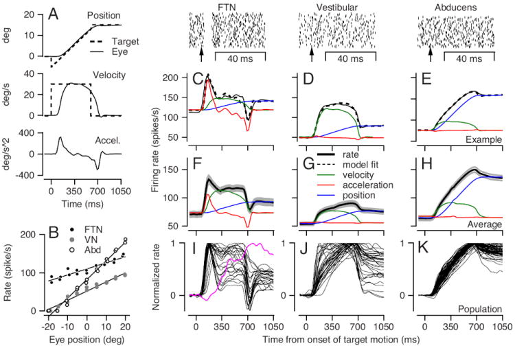
A: Eye movement behavior during step ramp target motion. Solid and dashed lines show eye and target motion. B: Relationship between firing rate and eye position during 1 second of fixation. Each symbols shows one fixation trial; lines were obtained by regression. The data are plotted using positive values to indicate steady eye position in the preferred direction, which was ipsiversive for Abducens neurons, contraversive for most FTNs (see also Lisberger et al., 1994a), and about equally ipsiversive and contraversive for non-FTN vestibular neurons. C-E: The average response of an example FTN (C), vestibular (D) and Abducens (E) neuron during smooth pursuit. The black line illustrates the average firing rate across trials; the dashed line illustrates the best linear fit from Equation (5). The blue, green, and red lines represent the contributions of eye position, velocity, and acceleration to average firing rate. The rasters above each neuron show the response to 100 electrical stimulations in the floccular complex at the time marked by the vertical arrow. F-G: The average responses of the populations of neurons (black) and the average contributions of the different kinematic parameters to the total firing rate. I-K: Time-varying firing rate of individual neurons normalized for the peak. The purple trace in I is the only FTN dominated by eye position sensitivity. Only neurons with responses larger than 50 spikes/s are shown.

We recorded from areas of the brainstem that contain neurons responding in relation to eye movement and vestibular stimulation (Ramachandran and Lisberger, 2006, 2008). Floccular target neurons, or “FTNs”, were identified by the clear pause in firing at monosynaptic latencies after application of single shocks through an electrode implanted in the cerebellar floccular complex (raster above Figure 1C). Other eye-movement related neurons in the vestibular nucleus and the Abducens nucleus failed to show the same pause after stimulation of the floccular complex with single shocks (rasters above Figures 1D, E), but were categorized according the their distinctive firing patterns and their recording locations relative to the Abducens nucleus.

Components of time-varying responses of identified brainstem neurons

Neurons in the different populations had different temporal response properties. The firing rate of the example FTN in Figure 1C (continuous black trace) shows a clear transient at movement onset followed by sustained activity: this pattern reflects a relationship to eye acceleration and eye velocity. The firing rate of the non-FTN vestibular neuron in Figure 1D also shows sustained activity but lacks a transient at pursuit initiation, indicating a relationship to eye velocity but not eye acceleration. For both the FTN and the non-FTN vestibular neuron, firing rate drops rapidly when the eye stops moving at the end of the trial, but to a level that is higher than the initial rate because of a relationship between firing rate and the change in eye position during the trial. The firing rate of the Abducens neuron in Figure 1E increases gradually during the eye movement with no sign of a transient at pursuit initiation and only a small decrease when the eye stops moving and settles at its final position at the end of the trial. Thus, Abducens neurons discharge mainly in relation to eye position, with smaller components related to eye velocity and eye acceleration (see Keller, 1973). The average firing rates across all neurons in each of the three categories (Figures 1F-H) agreed well with the individual examples (Figures 1C-E).

To follow the traditional approach of separating each neuron’s response into terms that represent the contributions of average eye acceleration, eye velocity and eye position, we fitted the time-varying average firing rate of each neuron with a linear model that represents firing rate as a weighted linear sum of instantaneous eye position, velocity, and acceleration:

$$\mathit{fr}(t)=a\ddot{E}(t-\mathrm{\Delta }t)+r\dot{E}(t-\mathrm{\Delta }t)+\mathit{kE}(t-\mathrm{\Delta }t)+\mathit{rr}$$ (5)

Here, rr is firing rate during fixation at straight ahead; Δt indicates the time shift of the eye movement averages need to optimize the fit to the average firing rate; a, r, and k represent the sensitivity of the neuron to eye acceleration, velocity, and position; and aË(t), rĖ(t), and kE(t) represent the contributions of average eye acceleration, eye velocity and eye position to firing rate (colored traces in Figure 1C-H).

As shown by others (Keller, 1973; Fuchs et al., 1988; Scudder and Fuchs, 1992; Shidara et al., 1993; Sylvestre and Cullen, 1999; Medina and Lisberger, 2007), fitting the average responses with Equation (5) provides a reliable account of the neural responses. The percentage of the variance accounted by the fit was 88%, 99.1%, and 99.9% for the neurons illustrated in Figure 1C, D, and E, and averaged 88%, 89%, and 99.5% across our full samples of FTNs, vestibular, and Abducens neurons. Comparison of the actual and predicted firing rate in Figure 1C (black continuous and dashed curves) provides a sense of the quality of a fit that accounts for 88% of variance. We inspected all fits to ensure that there were no major systematic errors for any of the individual neurons in our sample.

The transient increase in the FTN response at the initiation of movement and the transient decrease at movement offset reflect a large contribution of the eye acceleration component (red trace in Figure 1C and F). Typically FTNs showed a brisk initial rise in firing rate at the onset of pursuit, and most showed a transient response with sustained responses that varied in magnitude across the sample. Only one FTN (Figure 1I, purple trace) showed a large ramp increase in firing rate during pursuit, as might be expected from a relationship to eye position that would result from neural integration.

The steady response of non-FTN vestibular neurons across the duration of the eye motion reflects the large eye velocity component (green trace in Figures 1D and G). Very few vestibular neurons (Figure 1J) showed the early transient typical of FTNs, but many showed some degree of ramp increase in firing across the duration of the response to step-ramp target motion. Thus, there was impressive diversity in the magnitude of the integrated response in vestibular neurons. Later in the paper, the diversity of the responses of non-FTN vestibular neurons will help constrain possible neural circuit mechanisms of integration.

The ramp increase in firing rate of Abducens neurons, with little decrement when eye motion stops, reflects the dominance of the eye position component of firing rate (blue trace in Figure 1E and H). The population of Abducens responses (Figure 1K) was impressively uniform, and all neurons showed a large ramp of firing rate throughout the ramp change in eye position for step-ramp target motion. Thus, Abducens neurons uniformly emit an integrated response. Abducens and non-FTN vestibular neurons showed response components related to both eye position and eye velocity, but the ratio of the maximal contribution of the position versus velocity signals was higher in Abducens neurons (2.82) than in vestibular neurons (1.05) (see also Scudder and Fuchs, 1992).

The differences in the contributions of the different components of eye movement to the firing of different classes of neurons appeared clearly in the resulting values of the sensitivity to eye acceleration, velocity, and position (scatter plots of Figures 2A and B). For example, Abducens neurons (blue symbols) had quite large sensitivity to eye position shown by the wide spread on the x-axis, but very little sensitivity to eye acceleration shown by the horizontal relationship in Figure 2A. In contrast, FTNs (red symbols in Figures 2A and B) had large sensitivity to eye acceleration and smaller sensitivity to eye position, shown by the nearly vertical relationship in Figure 2A. Vestibular neurons (green symbols) also had little sensitivity to eye acceleration and plotted in a mostly horizontal clump with sensitivities to eye position that were smaller than those of Abducens neurons. Comparison of sensitivity to eye velocity and position (Figure 2B) revealed a steeper slope in FTNs and vestibular neurons versus Abducens neurons, indicating more of an emphasis on eye velocity signals outside the Abducens nucleus and more emphasis on eye position in Abducens neurons.

Figure 2. Sensitivity of different groups of neurons to the parameters of eye movement.

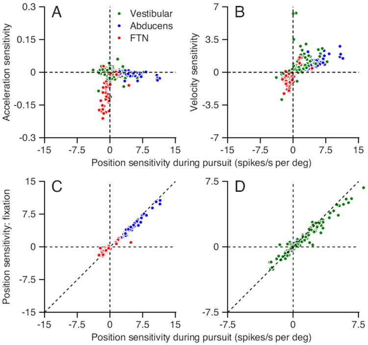
Each symbol shows the response of an individual neuron; red, green, and blue dots represent FTNs, vestibular neurons, and Abducens neurons A: Eye acceleration versus position sensitivity. B: Eye velocity versus position sensitivity. All values of sensitivity from Equation (5). C-D: The slope of the regression line relating firing rate to steady eye position during fixation versus position sensitivity during smooth pursuit trials, from Equation (5). Dashed diagonal line illustrates the unity line. Positive values of sensitivity correspond to increases in firing rate for eye movements toward the side of the recording.

We found a relatively small sensitivity to eye acceleration in the “EHV” vestibular neurons that lacked inhibition by floccular stimulation but had the same responses in relation to sinusoidal eye and head movements as did identified FTNs (Scudder and Fuchs, 1992). Sensitivity to eye acceleration was almost 6 times larger for FTNs than for EHV neurons (0.095 versus 0.016 spikes/s per deg/s², p < 0.001, t-test on absolute values). Thus, we suggest that their cerebellar inputs cause the sensitivity of FTNs to eye acceleration; previous studies that did not find an acceleration signal in EHV neurons probably sampled few or no FTNs (Roy and Cullen, 2003). We will elaborate about this difference between FTNs and EHV neurons later.

Eye position sensitivity during pursuit

We observed two manifestations of a relationship between eye position and firing rate in brainstem neurons. 1) Regression analysis with Equation (5) quantified the size of an eye position component during pursuit that also was responsible for the change in steady-firing rate that persisted at the end of pursuit. 2) Steady fixation for durations of 1 second or more revealed a relationship between steady firing and eye position (Figure 1B). Here, the large and small slopes of the relationships for the Abducens neuron (open symbols) and FTN (filled gray symbols) are correlated with the large versus small difference in steady firing rate between the start and end of pursuit of step-ramp target motion (Figures 1F versus H).

To test quantitatively the similarity in the sensitivity of the cells in the different conditions, we plotted the slope of the relationship between firing rate and eye position during steady fixation (Figure 1B) as a function of the value of the position sensitivity during pursuit, obtained from Equation (5). For all three classes of neurons, the sensitivity to eye position was only slightly larger during pursuit than during fixation (see also Fuchs et al., 1988), as indicated by the tendency of cells to plot slightly above and below the equality line in the first and third quadrants in Figures 2C and D. The consistent position sensitivity of the cells across conditions suggests that there is a single common source of the eye position component of firing of brainstem neurons.

We showed that the position signal during pursuit is not subsequent to a fast decay of firing rate after saccades by comparing the sensitivity to eye position from Equation (5) between averages from trials with versus without saccades. The estimates of sensitivity to eye position were effectively equal (r> 0.995). We also quantified the persistent change in firing rate at the end of pursuit trials for a subset of neurons where we obtained up to 650 ms of fixation after target motion offset. We observed little decay in firing rate over 650 ms of fixation, implying that the time constant of decay must be very large, if there is decay at all. The sensitivities to eye position from Equation (5) again were almost equal whether we used 300 or 650 ms of post-pursuit steady fixation (r>0.992). Thus, we find it difficult to attribute the eye position component of the time-varying firing rate during pursuit to other sources, such as a rebound from a saccade, or components related to eye velocity or eye acceleration.

Diversity of time-varying firing rate profiles

The time-varying firing rates of the neurons in our sample aligned with the traditional definition of different classes of brainstem neurons to some degree, but incompletely. In Figure 3, we have broken our sample of neurons into FTNs, EHV neurons, PVP neurons, eye-only neurons, and Abducens neurons, and we have plotted the normalized firing rate on a color scale as a function of time on the x-axis; each individual neuron is shown as one horizontal line. Ordering the cells from bottom to top according to the time of the peak firing rate allows clear visualization of the diversity (or not) of time varying firing rate within each group, and the differences across groups. FTNs show strong transients in many neurons, and the peak firing rate almost always occurred at the start of the pursuit response. At the other extreme, Abducens neurons show uniform responses that reflect integration; they ramp up gradually to peaks that occur near the end of the pursuit response. Non-FTNs recorded in the region of the vestibular nucleus had quite diverse time-varying firing rates. Some EHV neurons had transient responses at the onset of pursuit, but the majority reached peak firing in the second half of the pursuit response. PVP neurons showed a wide range of responses with peak firing reached at times that were uniformly distributed across the second half of the pursuit response. The eye-only neurons tended to reach peak firing rate quite late in the response.

Figure 3. Time-varying responses of neurons separated according to standard classification into different functional response patterns.

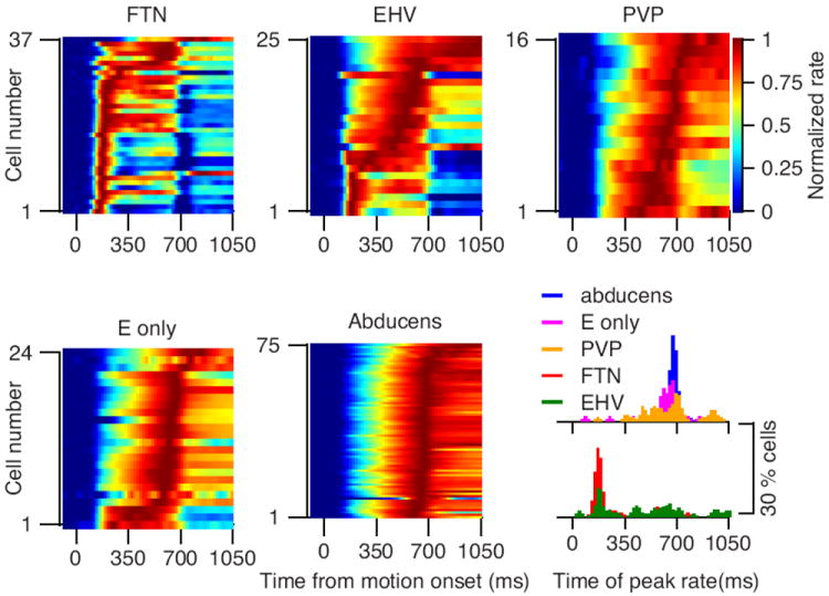
In each color image, a horizontal line plots the response of one neuron as a function of time, different neurons are stacked vertically, and color shows the normalized firing rate. Neurons with responses larger than 25 spikes/s were included. The histograms at the lower right plot the time when peak firing rate was reached. Different colors indicate neurons categorized according to their functional firing patterns during eye movement and vestibular stimulation. Histograms were calculated with all neurons and smoothed with a moving average of 2 bins (40 ms).

The distributions of the time of peak firing in different classes of neurons (Figure 3, bottom right), and statistical analysis with ANOVA and the Tukey post hoc test, support the statements made above. FTNs were the first to reach peak firing rate at 278 ms (p<0.05). The second to peak were EHV neurons at 486 ms (p < 0.05). The last three populations tended to reach peak firing towards the end of the trial and the difference between the populations did not reach significance (600, 648, 692 for EM, PVP and Abducens neurons). Thus the sharpest difference was between FTNs and other cells in the vestibular nucleus but with a progressive transformation from FTNs to EHV cells and then to PVP and EM cells.

Transformations of cerebellar outputs into motoneuron responses

Our ultimate goal is to determine how neural circuits transform from the time-varying firing rates of Purkinje cells (PC) in the floccular complex of the cerebellum to the time-varying firing rates of Abducens neurons. Two questions need to be answered as the next step towards our goal: 1) How must the outputs of floccular Purkinje cells be modified to create the time-varying firing rates of FTNs? 2) How are the outputs of FTNs and other vestibular neurons combined and transformed to create the time-varying firing rates of Abducens neurons?

We ask how Purkinje cell outputs are transformed to create the activity of FTNs by comparing our recordings from the brainstem with those from a previous study of the activity of Purkinje cells in the floccular complex during pursuit of step-ramp target motion (Medina and Lisberger, 2007, 2009). To take into account the facts that Purkinje cells inhibit FTNs and all neurons have high spontaneous firing rates, we examined the activity during pursuit in both the on- and off-directions for 38 FTNs with horizontal preferred directions and 36 PCs that preferred pursuit toward the side of the recording; we presume most of the PCs were “HGVPs” (Lisberger and Fuchs, 1978a). Both groups of neurons showed strong asymmetries, both for individual neurons (not shown) and for averages across the full samples (Figures 4A, B). Increases in firing rate for pursuit in the on-direction were generally larger than decreases in firing rate for pursuit in the opposite, off-direction (see also Krauzlis and Lisberger, 1994; Lisberger et al., 1994c).

Figure 4. Transformation from floccular output to FTN responses.

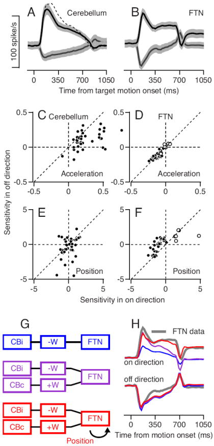
A-B: Average population activity of floccular Purkinje cells (PCs) and FTNs during smooth pursuit. Black and gray lines illustrate activity in the on and off directions and gray bands around the lines show the standard error of the mean (SEM). C-F: Sensitivity to eye position and acceleration in the off- versus on-direction for PCs (C, E) and FTNs (D, F). Each dot represents the sensitivity of one neuron and the dashed line illustrates the unity line. G: Schematic representation of three different models for creating the time-varying FTNs rate. Boxes represent cerebellar activity from the same (CBi) and opposite side (CBc) relative to FTN location, the weighing of the signal from the cerebellum (+W or −W), and the response of the FTN. H: The colored traces show the best fit for the three different models and the gray trace illustrates the average firing rates of FTNs. Top and bottom sets of traces are for the on- and off-directions.

PCs and FTNs acquired asymmetries from different sources. Based on the values obtained by the regression fits using Equation (5), the asymmetry in the simple-spike firing rate responses of PCs arose from a pronounced asymmetry favoring the on-direction for eye acceleration (Figure 4C); in contrast, FTNs showed nearly symmetrical sensitivities to eye acceleration (Figure 4D). The asymmetry in the firing rate responses of FTNs arose mainly from an asymmetry in position sensitivity, at least for the predominant population of FTNs that showed increased responses for eye movement away from the side of recording (Figure 4F). These showed the expected negative sensitivities to eye position for on-direction pursuit and much smaller negative sensitivities or even wrong-way positive sensitivities for off-direction pursuit (Lisberger et al., 1994a). Unlike the FTNs the PCs did not have a consistent position signal in the on- or off-direction, as indicated by the scatter of the cells around the origin in Figure 4E. Both groups of neurons showed slightly larger velocity sensitivity in the on- versus the off-direction (not shown).

To understand the neural circuit mechanisms that could create the discharge of FTNs from that of floccular PCs during pursuit, we explored the three schematic models in Figure 4G. From top to bottom, the models create FTN firing through:

1. unilateral inhibition from the ipsilateral floccular complex (blue model):

   $$\mathit{FTN}(t)=(-W·{\mathit{Cb}}_i(t))$$ (6)
2. opponent inhibition and excitation from the ipsilateral and contralateral floccular complex (purple model):

   $$\mathit{FTN}(t)=W({\mathit{Cb}}_c(t)-{\mathit{Cb}}_i(t))$$ (7)
3. the opponent mechanism plus position signals that are not present in the average outputs from the floccular complex of the cerebellum (red model):

   $$\mathit{FTN}(t)=W({\mathit{Cb}}_c(t)-\mathit{Cb}{(t)}_i)+\mathit{kE}(t)$$ (8)

   where FTN(t) is the figuring rate of FTNs as a function of time, Cb_i(t) and Cb_c(t) are the average firing rates of the floccular Purkinje cells on the same and opposite side relation to the FTNs, and E(t) is eye position as a function of time applied only in on direction of FTNs. We tested each model with the time-varying average firing of PCs as the input to the model and the time-varying average firing rate of FTNs as the output, by using linear regression to obtain the values of the scalar weights W and k that provided the best fits. For pursuit toward the side of one floccular complex, we assumed that PCs in the contralateral floccular complex would discharge with the same time-varying firing rates as ipsilateral PCs during pursuit in the off-direction (and vice versa).

As illustrated in Figure 4H, the model with the opponent mechanism and eye position signal (red traces) provided the best account of the actual responses of FTNs (gray traces) for pursuit in the on-direction and the off-direction, while the model without position signal (purple traces) predicted the data slightly more poorly. The unilateral model (blue traces) was unsuccessful. Figure 4H shows the results of simulations where the magnitudes of the weights were equal for the inputs from the two sides of the cerebellum. The outcome of the simulations was the same when we allowed the two weights to vary independently.

We think that PCs acquire an eye acceleration asymmetry from their visual mossy fiber inputs (Miles and Fuller, 1975; Noda, 1981; Stone and Lisberger, 1990), and that FTNs acquire their eye acceleration sensitivity from PCs. We suggest that FTNs have symmetric sensitivities to eye acceleration because of an opponent organization that compensates for the asymmetry in their direct floccular inhibition. We are not suggesting that FTNs receive monosynaptic inhibition from Purkinje cells on both sides of the brain, but rather that multisynaptic pathways might transmit signals from the contralateral floccular complex (or from other pursuit-related areas). The contralateral signal could arise from pathways that include the frontal eye field (Ono and Mustari, 2009), the reticular formation (Ono et al., 2004), the cerebellar vermis (Dash et al., 2012), or the caudal fastigial nucleus (Noda et al., 1990; Fuchs et al., 1994; Omori et al., 1997). We suggest that FTNs acquire an asymmetry in eye position sensitivity through asymmetric inputs from bilateral neural integrators (Aksay et al., 2007).

We turn next to the question of how the time-varying firing rates of Abducens neurons can be created from the time varying firing-rates of FTNs and other vestibular neurons. Prior work has emphasized the concepts that FTNs and other vestibular neurons project to motoneurons in parallel (Scudder and Fuchs, 1992; Lisberger et al., 1994b) and that cerebellar output must be subjected to neural integration for smooth pursuit eye movements (Shidara et al., 1993; Krauzlis and Lisberger, 1994). Figure 5 verifies the need for integration using three schematic models that, from top to bottom:

1. uses a single weight from both FTNs and vestibular neurons to Abducens neurons without integration (blue model):

   $$\mathit{Ab}(t)=W(\mathit{FTN}(t)+\mathit{VN}(t))$$ (9)
2. uses different weights from FTNs and vestibular neurons to Abducens neurons without integration (purple model):

   $$\mathit{Ab}(t)=W_1\mathit{FTN}(t)+W_2\mathit{VN}(t)$$ (10)
3. inserts a mathematical integrator between FTNs and Abducens neurons (red model):

   $$\mathit{Ab}(t)=W_1\int \mathit{FTN}(t)\mathit{dt}+W_2\mathit{VN}(t))$$ (11)

   where Ab(t), VN(t), and FTN(t) are the average firing rates of Abducens neurons, non-FTN vestibular neurons, and FTNs, respectively. Again, we used the time-varying average firing rates of FTNs and non-FTN vestibular neurons as the input to the models and the time-varying average firing rates of Abducens neurons as the output from the models. We used linear regression to find the values of the scalar constants W, W₁, and W₂ that provide the best fits of each model.

Figure 5. Transformation from FTN and vestibular firing to Abducens responses.

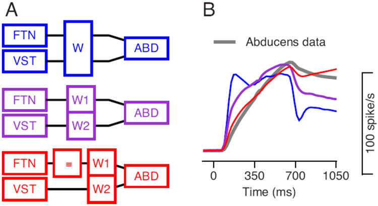
A: Three models for brainstem processing. The boxes represent the responses of FTNs and vestibular neurons (VST), weighting (W, W1, W2) or integration (Idt) of signals, and the responses of Abducens neurons (ABD). B: The colored traces show the best fit for the three different models and the gray trace illustrates the average firing rates of Abducens neurons.

The model that inserts a mathematical integrator between FTNs and Abducens neurons (Figure 5A, red model and Figure 5B, red trace) predicts firing that mimics the Abducens data (gray trace) well (r²=0.98). In contrast, neither the model that uses a single weight for the signals from both FTNs and vestibular neurons (blue model and traces) nor the model that uses separate weights without integration (purple model and traces) predicts Abducens firing rates that mimic the average from our data (gray trace, Figure 5B). We fitted these models with the weights as free parameters: the best fit for the integration model used weights of 2.14 and 1.03 for the vestibular and FTN pathways, indicating that both pathways are needed for the best performance of the model. Close inspection of Figure 5B reveals a minor transgression of the integrating model: because it integrates the eye position relationship of FTNs, it predicts (red curve) a small increase in Abducens firing rate that does not occur in the data (gray curve) when eye position is stable after the end of target motion.

The results presented in Figure 4 imply that FTNs provide inputs to, and are therefore upstream from, integration. On the other hand the results presented in Figure 5 imply that the large position signal in the FTNs must arise from the integrator, because the position signal is not available in the floccular complex. Therefore, FTNs seem to be downstream from the integrator. A group of neurons that both feeds into the integrator and receives feedback from the integrator is effectively a part of the integrator. We next study models that include FTNs as part of the integrator.

A neural model for brainstem computations

Our final goal was to understand how the diversity of time-varying firing rates of brainstem neurons, as well as the differences between different groups of neurons, constrain the implementation of neural integration by a neural circuit in the primate brainstem. Prior models have used a recurrent structure like the one we have explored (e.g. Cannon et al., 1983; Galiana and Outerbridge, 1984; Seung, 1996; Miri et al., 2011) and our goal was to go a step further and constrain the details of the recurrent connections. As detailed below, we find that the architecture of the recurrent connections suggested by Miri et al. (2011) has considerable explanatory power for the diverse time-varying responses of FTNs, vestibular neurons, and Abducens neurons of monkeys.

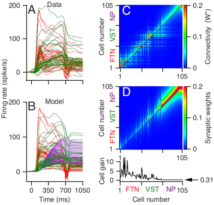
The most successful network had the general structure illustrated in the cartoon of neural connections in Figure 6A, chosen to follow the connections of the primate brainstem oculomotor structures as best they are known. We will revisit the degree of realism of the model in the Discussion. The model has a “soft” feed-forward architecture (Figure 6B): self-connections do not exist (Figure 6C, black pixels on the diagonal), and forward connections (above the diagonal) are stronger than feedback connections for all model neurons except those at the end of the hierarchy.

Figure 6. Hierarchical model of the brainstem neural integrator.

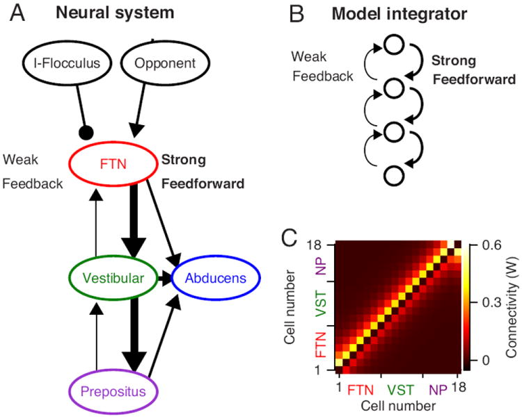
A: Schematic representation of the network. Each ellipse represents a population of neurons, arrows are excitatory connections, and lines ending with a circle represent inhibitory connections. The width of the arrows represents the strength of the connections. B: The architecture of a neural integrator suggested by Miri et al. (2011). Each open circle represents a single neuron or group of neurons, and the arrows represent connections. Each neuron is connected strongly the next neuron and weakly to the previous neuron. C: The colors indicate the connection weights in the connection matrix (W) between neurons for a network with soft feed-forward connections.

Model neurons #1-6 are intended to represent FTNs; they receive an external input equal to the average time-varying opponent firing rate we recorded in PCs. To calculate the input to the network we obtained the average sensitivities of floccular PCs to eye acceleration, velocity, and position (e.g. Medina and Lisberger, 2009), and used Equation (5) to generate the predicted firing rate of the cerebellar output for the actual behavior of the monkeys during recordings from brainstem neurons. We subtracted the predicted firing rate of PCs for movement in the off-direction from that for movement in the on-direction to create the opponent firing that served as the input to the network. Units #7-12 and #13-18 are intended to represent vestibular neurons and neurons in the nucleus prepositus (McFarland and Fuchs, 1992), and do not receive direct cerebellar inputs.

The model represented by the connectivity matrix in Figure 6C could reproduce the time course, but not the magnitude of the firing rates of the different neurons in the monkey’s brainstem. We achieved excellent agreement with both the amplitude and time course of the average responses of all 4 neuron types by using a procedure described in the Materials and Methods to adjust the internal gain of each population. Figure 7B shows the effective connectivity matrix resulting from this procedure. The connectivity matrix can be factored to show internal gain and synaptic connectivity separately while maintaining stronger feed-forward synaptic connectivity (Figure 7C). The resulting internal gain function is consistent with the biological finding that the gain of FTNs to injection of depolarizing current is larger than the gain for other vestibular neurons (Sekirnjak et al., 2003; Shin et al., 2011). In our model, the weight of a model neuron’s connection to the Abducens neurons is inversely proportional to its internal gain (Equation 4). Model FTNs are connected to the output to comply with anatomical findings (Shin et al., 2011), but have weak connections because they have large internal gains. As a result, the Abducens neurons do not follow the transient responses of FTNs at the onset of pursuit eye movement (Figure 4).

Figure 7. Comparison of average responses of real and model neurons.

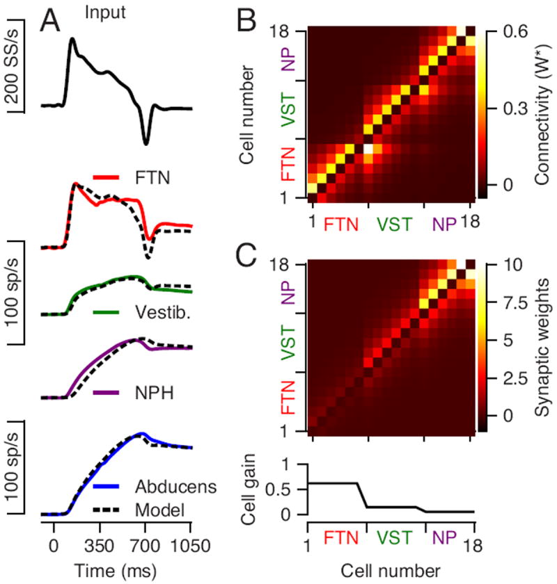
Dashed black and continuous curves illustrate the output from the model and the average firing rate of the data A: Continuous traces show average responses from our data and dashed traces show the output of an optimized model. From top to bottom the traces are: the input to model neurons #1-6 (FTNs), the average responses of FTNs, non-FTN vestibular neurons (model neurons #7-12), NPH neurons (model neurons #13-18), and Abducens neurons. We generated the activity of prepositus neurons according to their average sensitivity to eye kinematics in McFarland and Fuchs (1992). B: The colors show the effective connection strengths (W*) in the connection matrix between model neurons for a network that matches both temporal pattern and response amplitude. C: The colors in the image show the synaptic weights (referred to as W_synapse in the Methods) and the graph at the bottom shows the internal gain of each model neuron. The gain values are: g_FTN = 0.62; g_VST = 0.14 g_NPH = 0.05.

The properly-tuned simulation reproduced the average time-varying responses of the brainstem populations, including the early transient of FTNs, the sustained response of vestibular neurons, and the ramp increase in firing of prepositus and Abducens neurons (compare continuous and dashed traces in Figure 7A). Because we did not record in the nucleus prepositus, we used the data from McFarland and Fuchs (1992) to compute the time-varying firing rate the model was required to match. Note that the network model of Figure 7, unlike the lumped integrator model of Figure 5A, did not integrate the position component of FTN firing and, as a result, did not predict an increase in the firing of Abducens neurons during fixation at the end of the step-ramp target motion.

The models represented by the connectivity matrices in Figure 6C and 7B integrate perfectly because they satisfy the requirement that the largest eigenvalue of the connectivity matrix is one (Seung, 1996). Because many other connectivity matrices also would lead to integration, our next important step is to show that the diversity of time-varying firing rates in our data constrain the workable connectivity matrix to have the soft feed-forward configuration.

The model represented by Figures 7B and C reproduces the diversity of time-varying responses of different brainstem neurons. Of the 18 model units, units #1-6 (Figure 8B, red traces) show rapid rises and early transients during the initiation of pursuit, much as we found in FTNs (Figure 8A, red traces). Units #7-12 (green traces) show a diversity of rise times and sustained responses much as we found in many vestibular neurons. Units #13-18 (purple traces) showed responses very similar to those of Abducens neurons, and resembled neurons recorded in the nucleus prepositus and adjacent areas (Escudero et al., 1992; McFarland and Fuchs, 1992), as well as some neurons we found in the vestibular nucleus. The “integrated” nature of the responses of the model prepositus neurons also agrees with finding of integrated signals during saccadic eye movements in prepositus neurons that project to the Abducens nucleus (Delgado-Garcia et al., 1989; Escudero et al., 1992).

Figure 8. Responses of model neurons for different connection matrices.

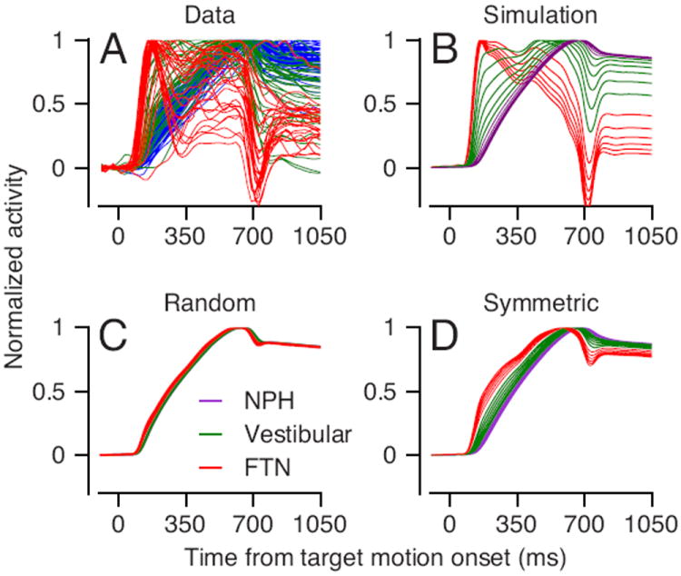
Each trace shows the time-varying firing rate of an individual neuron and different colors denote different groups of neurons. A: Data B: Model with strong feedforward and weak feedback connections. C: Model with connection strengths drawn randomly from a positive uniform distribution. D: Model with equal strengths of feedforward and feedback connections.

Many recurrent network architectures can perform neural integration, and our data provide constraints to narrow the range of possibilities. Our use of stimulation in the floccular complex to identify FTNs dictates a specific set of the connections to the input neurons of the integrator. Further constraints come from the need to simulate the diversity of the firing patterns in the vestibular neurons. If we allowed uniform but random connection weights between units, for example, the diversity of neural responses was lost and all model neurons showed the same, integrated, time-varying firing rate (Figure 8C). Increasing or decreasing the mean value of the random weights caused the output of the model to increase or decrease exponentially when it was supposed to be steady, but did not create more diversity in the time-varying responses of the model neurons. If we created symmetry in the feed-forward and feedback connection weights, then much of the diversity of time-varying neural firing rates was lost, and early transient response in the responses of FTNs did not appear in the simulations (Figure 8D).

A number of alternate models have the same performance as the soft feed-forward architecture we have used, in the sense that they produce an integrated output and reproduce the diversity of time-varying firing rate found in brainstem neurons. For example, very similar results emerge from a network with feed-forward connections from unit to unit and a single feedback connection from one unit to the whole network. Also, it is possible to reproduce the model’s performance with a set of internal weights that are uniformly random and a progression of time constants in the model neurons, from very short for the model FTNs to longer for other neurons in the integrator. The model with diverse time constants is equivalent to a model with uniform time constants and self-inhibitory connections. Thus, inhibition might also be important for generating diverse responses.

Finally, we scale-up our small model network and show that a larger network can reproduce the time-varying responses of a larger number of individual neurons from our recording sample. Now, we use a network with 105 model neurons, increasing the width of the connection matrix accordingly (see Methods), and we adjust the synaptic weights and the internal gains so that our model units match the responses of 35 FTNs and 35 vestibular neurons selected randomly from our sample (Figures 9A, B). The successful model used a weight matrix and internal gains (Figure 9C) that are noisier, but follow the same patterns as those in the smaller network model we used to establish proof of principle (Figure 7C). All 35 model prepositus neurons in this version of the model had the same synaptic weights and internal gains, because we modeled them all to match a single average firing rate calculated using the parameters of Equation (5) from McFarland and Fuchs (1992).

Figure 9. A network model that integrates and reproduces the time-varying firing rates of a large sample of brainstem neurons during smooth pursuit.

A: data. B: model neurons. Red, green and purple thin lines show deviation from baseline firing rate of FTNs, vestibular neurons, and prepositus (model only) neurons. C-D: The color images show the effective connection matrix (W*) and the synaptic connectivity (referred to as W_synapse in the Methods) for all 105 model neurons in the network. The graph at the bottom shows the internal gain of the different model neurons.

Effects of selective lesions of hierarchical integrator models

To study how different cells contribute to integration in our model network, we reduced the synaptic weights at individual model neurons to 95% of the weights that lead to perfect integrations thereby “lesioning” the hierarchical network at different stages of processing. Even a lesion of a single model neuron causes the network to integrate imperfectly, so that it will decay from any initial state to zero. We tested the network by setting the state of all the neurons to the same, non-zero value and running the simulation with no further input. Lesions of model neurons at the top of the hierarchy cause a slow decay in the output of the network (Figure 10A, red curves). Lesions of model neurons that are closer to the end of the hierarchy (green and purple curves) cause faster decays in activity. Thus, the entire network contributes to integration with a larger proportion of the integration done in the bottom of the hierarchy. The hierarchical network is more robust to perturbation at the top of the hierarchy.

Figure 10. The effect of lesions on the model output.

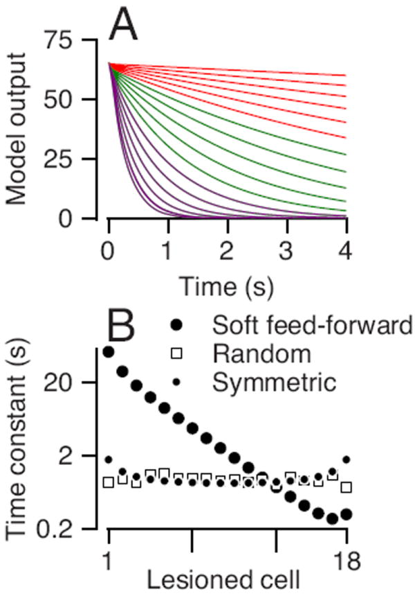
A: Each trace shows the output of a hierarchical network when the weights of one of the cells are decreased to 95% from perfect integrations. Colors denote the group of the cell with the reduced weight: red indicates model units #1-6, green indicates model units #7-12, purple indicates model units #13-18. B: The time constant of the decay in activity as a function of the number within the hierarchical network of the cell that was lesioned. Open circles, open squares, and filled circles show results for the networks with stronger feedforward connections, uniformly random connections, and symmetric connections.

We quantified the contribution of each model neuron to integration and compared contributions in different models by calculating the time constant of the exponential decay for lesions as a function of the location of the model neuron in the integrator circuit. In the hierarchical soft feed-forward model, the decay in the output decreased with the number of the lesioned cell (Figure 10B, open circles). In the networks with random, uniform connections between model neurons, the time constant of the decay was independent of the location of the model neuron (Figure 10B, open squares), indicating that all neurons contribute equally to the integration. In the hierarchical network with symmetrical feed-forward and feedback connection weights, the time constants of the neurons in the middle of the network were slightly smaller indicating that they made a slightly larger contribution to integration.

The pattern of feedback connections, but not the gain factors, determine the relationship between the time constant of the decay after lesions of single model neurons and the location of the lesioned neuron in the hierarchy. In the hierarchical model, the strongest feedback weights accrue at the end of the hierarchy and lesions in these model neurons lead to leakier integrators, which is consistent with previous studies that emphasized the role of prepositus in integration (Fukushima et al., 1992). Reducing the asymmetry between feedforward and feedback, thereby increasing the strength of the feedback in the top of the hierarchy, leads to smaller differences in the time constants of decay. On the other hand, changes in the internal gains of the model neurons does not change the time constant of the network decay: lesions to the same model neuron in networks with weights W or W* leads to the same time constant in the decay of the network output. The similarity occurs because the lesioned networks have the same eigenvalues and hence same decays in output activity.

Figures 8 and 10 provide an intuition about why the pattern of connections affects the predictions for the time-varying responses of different neurons. When the connection matrix is random and uniform, all model neurons operate as equals, and they are effectively clamped together so that they all show the same time-varying response patterns. When lesions reduce the integrating capability of the network, the responses of all model neurons decay at the same rate. If the feed-forward and feedback weights are symmetrical, then the integrated output of the network is fed back strongly to the input layers and it overwrites the time-varying pattern in the inputs to the integrating network. Only if the feed-forward weights are stronger than the feedback weights can the inputs dominate the integrated feedback at the top of the network. In a similar fashion, the inputs from higher in the hierarchy have a stronger influence on each model neuron than do the feedback connections, so that integration occurs progressively as the signals pass through the hierarchy.

One model can reproduce the responses of integrator neurons in zebrafish and monkey

The structure of our most successful model is derived from one of the models used by Miri et al. (2011) to account for their data on the responses of neurons in the brainstem of larval zebrafish during eye fixations. There are two main differences between our model and theirs. First, Miri et al. (2011) used a model that did not integrate perfectly so that they could reproduce the decays in eccentric eye position in their data; we set the recurrent weights in the model to act as a perfect integrator because the time constant of the decay of eye fixations is very long in primates (Becker and Klein, 1973). Second, Miri et al. (2011) used model neurons with time constants of 1 second; we used a short neural time constant of 5 ms because using a single long time constant prevented model FTNs from displaying the transient response seen in the real FTNs.

We explored the operation of both models by setting the activity of all model neurons to have a value of one at the start of a simulation, and then exploring how the activity of the model neurons evolved to a stable state. In Figures 11A and B, the models for both species were set to achieve perfect integration and their net outputs were steady throughout the simulations (not shown). In both models, the model neurons reached diverse, but steady values before the end of the simulation. The model neurons in the “zebrafish” network required several seconds and followed diverse trajectories to final states, because of the long time constant of the individual model units. The model neurons in the “monkey” network reached a final, sustained value almost immediately, because of the short time constants of the individual model units. Even though the activity of the different neurons evolved over different time courses in the two models, the overall output of both models was constant because both were tuned to integrate perfectly.

Figure 11. Comparison of the responses of different model neurons in networks that used short and long time constants in the model neurons.

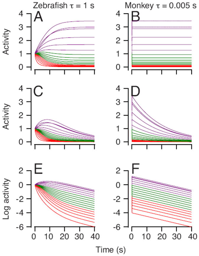
Each trace shows the time-varying firing rate of an individual neuron and different colors denote different groups of neurons: red indicates model units #1-6, green indicates model units #7-12, purple indicates model units #13-18. The left and right column show results from simulations with neural time constants of 1 and 0.005 seconds. A-B: Networks are tuned to produce perfect integration. C-D: Networks are tuned to have a decay time constant of 20 seconds in their overall output. E-F: Same as C-D, but the responses of the model neurons are plotted on a log scale.

Next we reduced the size of the connection weights uniformly so that the overall output from both models showed leaky integration with decay time constants of 20 seconds. Now, the model neurons in the “zebrafish” network (Figure 11C) showed a complex and diverse time-varying activity early in the simulation and more uniform decay later in the simulation; the progression of the two decays can be appreciated better in the log plots (Figure 11E), which show that the decay is linear and has the same time constant in all model neurons late in the simulation. In contrast, the model neurons in the “monkey” network (Figure 11D), snap quickly to an initial state and then decay at a constant rate that is the same in all model neurons, a feature that again is most visible in the log plots (Figure 11F).

In the simulations presented by Miri et al. (2011), the time constant of the model neurons and the architecture of the weight matrix together are responsible for the early part of each model neuron’s time-varying trajectory. Both are constrained by the need to account for the diversity of the time constants of decay in the calcium imaging data from the zebrafish. In our simulations of the data from the monkey brainstem, the diversity of the time-varying firing rates does not require the long time constants of the model neurons, and appears solely because of the soft feed-forward architecture of the weight matrix. Thus, the long time constant of 1-second used in the model neurons by Miri et al. (2011) is essential for the diversity in the decay of the calcium signals in the zebrafish, but not for the diversity in the time-varying responses in monkeys. Even with long time constants, however, the later parts of all model neurons’ responses decay at a uniform rate that depends on the time constants of the neurons. Thus, decay in the individual neurons in zebrafish would have collapsed to the single, uniform time constant expected of a line attractor if they had extended their recordings to longer fixations.

In simulations of the monkey data, we are able to see the consequences of the network architecture even with a movement of duration only 1 second because the behavior endures 200-fold longer than the 5-ms time constant of our model neurons. Miri et al (2011) observed diverse time constants of decay that are the consequences of the time constants of the model neurons because their behavior endured 5 seconds, only 5-fold longer than the time constant of their model neurons. A model with only short time constants cannot easily reproduce the zebrafish data, while a model with only long time constants cannot reproduce the monkey data. Still, the model network with short time constants in the model neurons is pertinent across a wide range of time scales. It allows gaze holding over a period of tens of seconds, and controls the eyes during one second of dynamic tracking behavior.

Discussion

The architecture of a neural integrator

The need for a circuit that implements a neural integration in the brainstem was recognized by analyzing gaze holding in primates (Robinson, 1964) and by comparing the activity in vestibular afferents and extraocular motoneurons of the monkey (Skavenski and Robinson, 1973). Yet, recordings from the brainstem of monkeys have largely failed to lead to conclusive evidence for any particular neural circuit implementation of integration. The responses of neurons are diverse, and seemingly without a “topography”. Thus, the localization (or not) of the neural integrator was driven by lesion studies showing that large areas in the brainstem that are essential for an intact neural integration (Cannon and Robinson, 1987; Cheron and Godaux, 1987).

The precision of its neural integrator makes the primate oculomotor system into the “acid-test” for integrator models. Yet, the monkey may not be the ideal preparation for the kinds of measurements needed to determine the exact architecture of a neural circuit that integrates. The detailed neural mechanism of integration may be demonstrated in preparations that afford large technical advantages for analyzing the relationship between circuits and behavior, but less impressive behavioral repertoires. But, to show its relevance to more complicated neural networks and rich behavior, any model will have to work across species so that it may reproduce the mean and variety of the time-varying responses of neurons in the monkey’s brainstem.

In the present paper, we propose a circuit mechanism for neural integration that links the pioneering recent advances of Miri et al. (2011) in understanding the architecture of a neural integrator with the traditional question of neural integration for control of eye movements in the brainstem of the monkey. Their study used modern microscopy to estimate neural activity in a putative integrating circuit in the brainstem of larval zebrafish. They were able to infer an important relationship between physical separation and connection strength of pairs of neurons in the circuit. Our study uses traditional single unit recording methods during a highly-repeatable specific behavior to show that a circuit proposed for the zebrafish reproduces a large body of neural responses in the oculomotor brainstem of the monkey.

The key principles of our model are: 1) the strong driving inputs from model Purkinje cells to FTNs effectively clamp the responses of the model FTNs in spite of their organization as part of a hierarchical integrator; 2) a hierarchical organization creates the diversity of neural responses we recorded in non-FTN vestibular neurons; and 3) weak feedback of the integrated signal creates diverse time-varying firing rates across the integrator while allowing some neurons (i.e. FTNs) to be part of the integrating circuit, show discharge in relation to eye position, and retain their time-varying firing in relation to the inputs to the neural integrator.

The convergence of the models from the two studies supports a plausible neural circuit implementation of neural integration that may be the same across a wide range of phylogeny, and across multiple brain areas and functions in primates. Neural integration performs the broader function of converting a transient signal into a sustained one, or converting a steady signal into a ramp increase in firing. It is possible, but not guaranteed, that the brain might use similar neural circuits to implement integration in the oculomotor brainstem, to create delay activity in the cerebral cortex (Romo et al., 1999), and to accumulate evidence leading up to a perceptual decision (Mazurek et al., 2003).

Relation to other models and data

Many investigators have suggested a recurrently connected neural circuit for integration (Cannon et al., 1983; Douglas et al., 1995) and recent work has suggested mechanisms for robustness of an integrator based on long time constants or thresholds in individual neurons (Seung, 1996; Seung et al., 2000; Koulakov et al., 2002; Goldman et al., 2003). Our work extends and refines these concepts in important ways. For example, it limits the utility of integration solely with intrinsic cellular time constants (Loewenstein and Sompolinsky, 2003) or purely feed-forward connections (Goldman, 2009) because these mechanisms would not allow neurons like the FTNs to show sensitivity to both eye position and acceleration. It mitigates in favor of a particular architecture of synaptic connections and strengths within the model integrator network, and suggests that much of integration is based on the properties of the network rather than the elements within the network.

Many elements of our model have parallels in the oculomotor circuitry. The floccular complex makes monosynaptic inhibitory synapses on a particular group of vestibular neurons know as FTNs (Langer et al., 1985; Lisberger et al., 1994a; Shin et al., 2011). The brainstem populations are interconnected (Belknap and McCrea, 1988) and both FTNs and non-FTN vestibular neurons connect to Abducens neurons (Scudder and Fuchs, 1992). Still, important aspects of our model have not been proven. Connections from FTNs and non-FTN vestibular neurons to the nucleus prepositus seem likely (Baker and Berthoz, 1975; Belknap and McCrea, 1988) but are not proven. Feedback connections from the nucleus prepositus to FTNs and non-FTN vestibular neurons seem plausible (Belknap and McCrea, 1988) but the specific connections proposed here have not been demonstrated. Most importantly, it is not known whether the connections have the proposed hierarchical architecture and soft feed-forward synaptic strengths. Finally, some features of brainstem anatomy are not included in the model, for example feedback from the brainstem to the floccular complex (Lisberger and Fuchs, 1978b; Miles et al., 1980; Belknap and McCrea, 1988) We think that these projections serve mainly to provide head and eye velocity signals to Purkinje cells (Lisberger and Fuchs, 1978b, a; Lisberger, 2010), but they also may provide the weak eye position signals found in some Purkinje cells and could have a role in neural integration.

An alternative explanation for our data suggests that brainstem neurons are not part of a distributed, hierarchical integrator. Instead, the diversity of time-varying responses in brainstem neurons could result from different weightings of eye velocity and eye position signals onto the different neurons. We think that this explanation is difficult to defend for FTNs and PVP neurons. These two groups of neurons relay signals that must be integrated to drive eye movement for smooth pursuit eye movements and the vestibulo-ocular reflex. Therefore, FTNs and PVP neurons almost certainly provide inputs to the integrator circuit. Because they have signals related to eye position, FTNs and PVP neurons also receive feedback from the integrator. Neurons that have feed-forward and feedback connections to the integrator, such as FTNs and PVP neurons, will operate as part of the integrator and their reciprocal connections with other integrator neurons will play a big role in determining the time-varying firing rates of FTNs and PVP neurons, as in our model. The same argument does not necessarily hold with the other neurons in our sample. For example, non-FTN vestibular neurons could receive velocity signals from FTNs and PVP neurons and position signals from the integrator, and project directly to motoneurons without sending outputs to the integrator. Thus, these non-FTN vestibular neurons could show a diversity of response properties simply because of different weightings of their eye velocity and eye position inputs, and not because they are part of an hierarchical integrator circuit.

Studies of the saccadic part of the brainstem provide some data that would support a model of integration similar to the one we have used. Prepositus neurons that project to the Abducens nucleus tend to discharge only in relation to eye position, while other neurons in the prepositus and vestibular nucleus discharge in relation to different combinations of saccadic eye velocity and position (Delgado-Garcia et al., 1989; Escudero et al., 1992). So far, the data on saccades has not been integrated into a computational neural model like ours. An interesting next step in monkeys would be to accumulate data on the discharge of individual neurons during saccades, pursuit, and the vestibulo-ocular reflex and determine whether a single integrator model like ours can account for the responses of brainstem neurons during all kinds of eye movements.

Our model has a number of limitations that we see as areas for future research. First, it does not include inhibition, which has an important role in brainstem computations (Shimazu and Precht, 1966; Gittis and du Lac, 2007) and might be an essential part of integration (Cannon et al., 1983). Second, the data we acquire on the monkey cannot test for the network organization proposed by Miri et al (2011), where connection strengths between neurons are related to the physical distances between them. Third, we did not separate Abducens neurons into motoneurons and internuclear neurons (Baker and Highstein, 1975; Fuchs et al., 1988; Sylvestre and Cullen, 1999); the uniformity of the Abducens responses implies that this is not a major issue. Fourth, we did not study neurons for long fixations at the end of pursuit, although they maintained their steady final firing rate for as long as we required the monkey to fixate. The model itself was tuned to integrate and it therefore was able both to reproduce the dynamic responses during pursuit and to maintain steady firing rate and support eccentric fixation indefinitely. Fifth, the model does not reproduce the diversity of the transient responses in FTNs, probably because we provided exactly the same input from the cerebellum to all model FTNs. Finally, we obtained data mainly for target motion at 30 deg/s; the linearity of the relationship between firing rate and eye movement in brainstem eye movement neurons (e.g. Fuchs and Kimm, 1975; Scudder and Fuchs, 1992) implies that the entire analysis will hold for other speeds of target motion as well.

Conclusions

The success of the integrator model suggests that the seemingly diverse collection of time-varying neural responses in the monkey’s brainstem would be expected of a distributed, locally-connected circuit like that suggested by analysis of the zebrafish brainstem. Still, confirmation of the exact neural mechanisms of integration is likely to come from a preparation that allows the kind of modern measurements already accomplished in the larval zebrafish. Thus, the contribution of our paper is the important step of illustrating that the neural models suggested by calcium imaging data in zebrafish provide a common solution to the same neural computation for both species. We also emphasize the possibility and necessity of finding ways to leverage the unique advantages of very different preparations such as the larval zebrafish and the awake monkey, to fully answer questions of the neural circuit mechanisms of complex behaviors.