

Abstract
Actions can be planned in either an intrinsic (body-based) reference frame or an extrinsic (world-based) frame, and understanding how the internal representations associated with these frames contribute to the learning of motor actions is a key issue in motor control. We studied the internal representation of this learning in human subjects by analyzing generalization patterns across an array of different movement directions and workspaces after training a visuomotor rotation in a single movement direction in one workspace. This provided a dense sampling of the generalization function across intrinsic and extrinsic reference frames, which allowed us to dissociate intrinsic and extrinsic representations and determine the manner in which they contributed to the motor memory for a trained action. A first experiment showed that the generalization pattern reflected a memory that was intermediate between intrinsic and extrinsic representations. A second experiment showed that this intermediate representation could not arise from separate intrinsic and extrinsic learning. Instead, we find that the representation of learning is based on a gain-field combination of local representations in intrinsic and extrinsic coordinates. This gain-field representation generalizes between actions by effectively computing similarity based on the (Mahalanobis) distance across intrinsic and extrinsic coordinates and is in line with neural recordings showing mixed intrinsic-extrinsic representations in motor and parietal cortices.
Introduction
During visually guided reaching, the sensorimotor system must estimate the spatial location of a target, the associated movement vector, and the motor output required to achieve it. The nature of the internal representation of this information is a key issue in understanding the mechanisms for sensorimotor control. The neural representation of the spatial information associated with the location of the target and the movement vector defines a coordinate system that determines the similarity with which the nervous system views different movements. In line with this idea, a series of studies have attempted to elucidate these representations by studying how learned changes in motor output generalize across spatial locations and motion states during reaching arm movements (Shadmehr and Mussa-Ivaldi, 1994; Ghahramani et al., 1996; Conditt et al., 1997; Conditt and Mussa-Ivaldi, 1999; Krakauer et al., 2000; Shadmehr and Moussavi, 2000; Morton et al., 2001; Baraduc and Wolpert, 2002; Malfait et al., 2002; Morton and Bastian, 2004; Smith and Shadmehr, 2005; Bays and Wolpert, 2006; Hwang et al., 2006; Ghez et al., 2007; Mattar and Ostry, 2007; Wagner and Smith, 2008; Haswell et al., 2009; Mattar and Ostry, 2010; Quaia et al., 2010; Gonzalez Castro et al., 2011; Joiner et al., 2011). As illustrated in Figure 1A, a change in the posture of the end effector allows for dissociation between intrinsic and extrinsic movement representations. Correspondingly, several studies have performed postural manipulations to explore the extent to which the neural coding of movement or the functional representations of motor memories are associated with coordinate systems intrinsic or extrinsic to the end effector. Studies in which novel physical dynamics were learned during reaching arm movements have generally found a representation for motor learning intrinsic to the end effector, in the joint coordinates of the arm (Shadmehr and Mussa-Ivaldi, 1994; Shadmehr and Moussavi, 2000; Malfait et al., 2002; Bays and Wolpert, 2006), whereas studies of visuomotor transformation learning have often suggested that the coordinate frame is based on position or motion extrinsic to the end effector (Vetter et al., 1999; Ghez et al., 2000; Krakauer et al., 2000).
Figure 1.

Experiment 1 diagram and theoretical framework. A, Task illustration. Left, Subjects adapt to a 30° VMR while reaching to a single target positioned in the 90° direction (trained direction), 9 cm away from the starting point. To move the cursor straight to the trained target (Trained cursor movement, solid black line), subjects need to perform a movement in the 120° direction (Trained hand motion, dashed green line). Middle, After learning the rotation, subjects performed reaching arm movements to an array of 19 probe targets (open gray circles), spaced 15° apart, spanning a range of −135° to +135° with respect to the trained direction in W1. Note that, in W1, the target at the 90° direction is the trained target, and therefore it corresponds to the trained target represented in both intrinsic and extrinsic space. Right, After learning the rotation, subjects also performed reaching arm movements to an array of probe targets (red circles) in W2, also spaced 15° apart. In W2, the extrinsic representation of the trained target is the target at 90° (yellow arrow), whereas the intrinsic representation of the trained target lies in the 45° direction (blue arrow). B, C, Ideal cursor movements to all targets in both workspaces. In B, movements are shown in extrinsic (Cartesian) coordinates, and in C, they are shown in intrinsic (joint) coordinates. InW1(gray), the black arrow shows the trained cursor movement. InW2(red), the yellow arrow shows the trained cursor movement in extrinsic space, whereas the blue arrow shows the trained cursor movement in joint space. Note that the black and yellow arrows are parallel in B, indicating that in Cartesian coordinates these two movements require the same position changes, whereas the black and blue arrows are parallel in C, showing that in joint coordinates those two movements require the same joint excursions. D, Target representations in I-E direction space. The x value for each movement is calculated as the distance between that movement and the trained movement in extrinsic coordinates. Similarly, the y value for each movement is calculated as the distance between that movement and the trained one in intrinsic coordinates. The intrinsic and extrinsic displacements from one target to the next are highly correlated within any particular workspace, yielding the nearly linear patterns forW1andW2shown in this panel (gray and red traces). E, Experimental protocol. The order of testing inW1andW2is randomized such that half the subjects were tested inW1first (top path) and half were tested in W2 first (bottom path).
Much of this previous work has assumed that each type of motor memory is encoded in a single reference frame, either intrinsic or extrinsic (Shadmehr and Mussa-Ivaldi, 1994; Vindras and Viviani, 1998; Ghez et al., 2000; Krakauer et al., 2000; Shadmehr and Moussavi, 2000; Malfait et al., 2002), and thus these studies were not designed to carefully examine the possibility that multiple coordinate frames might contribute to the internal representation of motor memory. However, more recent evidence suggests that novel dynamics are learned with a representation that is not fully intrinsic. For example, studies of children with autism (Haswell et al., 2009) and transcranial direct-current stimulation of motor cortex (Orban de Xivry et al., 2011) have found that disease or brain stimulation can lead to a significantly greater fraction of intrinsic generalization. However, this would not be possible if generalization were normally fully intrinsic, as previously suggested. Another recent study looked at the coordinate frame used in the representation of dynamics in tasks with visualizations of different complexity and concluded that physical dynamics are represented in a coordinate frame intermediate between intrinsic and extrinsic (Ahmed et al., 2008).
Despite the accumulating evidence that intrinsic and extrinsic coordinate frames both contribute to motor memory, little is known about the manner in which their contributions are combined. A key issue with previous work is that the sparsity with which these studies sampled the generalization of learning throughout the workspace did not allow for this level of investigation. Here we address this issue by measuring the generalization of visuomotor learning across an array of different movement directions and arm configurations, amounting to more than 50 conditions in total compared with the one or two untrained conditions examined in most previous studies. This dense sampling allows us to visualize the pattern of generalization across the combined intrinsic-extrinsic (I-E) space, revealing a representation of motor memory that arises from a gain-field combination of intrinsic and extrinsic coordinate frames. Importantly, our data distinguishes this multiplicative gain-field combination model from a previously assumed (Hikosaka et al., 2002; Cohen et al., 2005; Berniker and Kording, 2008; Berniker and Kording, 2011) additive combination model that corresponds to the idea of separate intrinsically based and extrinsically based learning. We show that this multiplicative gain-field model is consistent with the presence of intrinsic, extrinsic, and jointly I-E representations within posterior parietal cortex (PPC) (Andersen et al., 1985, 1998, 2004; Buneo and Andersen, 2006) and primary motor cortex (M1) (Kalaska et al., 1989; Kakei et al., 1999; Kalaska, 2009).
Materials and Methods
Participants
Thirty two right-handed subjects (13 men; mean age, 36.7 years) participated in this study. Twelve took part in experiment 1 and 20 in experiment 2. The subjects were naive to the purpose of the experiments, and all provided informed consent consistent with the policies of Institutional Review Board of Harvard University. Each participant took part in only one of the two experiments we conducted.
Apparatus
The configuration of the experimental setup is shown in Figure 1A. Subjects sat in a chair facing a 120 Hz, 23-inch LCD monitor, mounted horizontally in front of them at shoulder level, displaying the various visual cues during the experiment. Underneath the monitor, 8 inches below the face of the screen, a digitizing tablet (Wacom Intuos 3) was used to track and record the subjects' arm movements. Above the tablet, subjects held a handle containing a digitizing pen in their right hand, whose position was tracked by the tablet. The handle served two purposes: (1) it acted as a shell around the digitizing pen, increasing its diameter, making it more comfortable to grasp, and (2) it provided a wider contact surface with the tablet, promoting a more consistent vertical orientation of the pen. The handle had a flat bottom covered with Teflon (polytetrafluoroethylene) that lowered the contact friction, allowing it to glide smoothly on the tablet. The position data were recorded in real time (sampled at 200 Hz) using the Psychophysics Toolbox (Brainard, 1997; Kleiner et al., 2007) in MATLAB [version 7.10.0 (R2010a); MathWorks]. The resolution of the position data in the plane of the tablet was 0.005 mm, and the accuracy was 0.25 mm.
Experimental protocol
In this study, subjects performed 9-cm point-to-point reaching arm movements from a single starting location to 19 different target locations, as illustrated in Figure 1A. The starting location was a circle with diameter of 5 mm, and each target was a circle with 10 mm diameter. The cursor was also a circle with 2.5 mm diameter. Subjects performed this task in two distinct workspaces, and we conducted two experiments, with different pairs of workspaces as illustrated in Figures 1 and 4, respectively.
Figure 4.
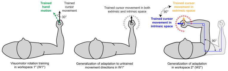
Experiment 2 diagram. Subjects adapted to a 30° rotation (left) before generalization was tested in 19 different movement directions in two distinct workspaces (middle and right) as in experiment 1. Note that here the trained workspace (W1*) is the same as the novel workspace (W2) in experiment 1, and the novel workspace in experiment 2 (W1*) is separated from W1* by +90° compared with the −45° separation in experiment 1.
Both experiments began with a block of trials in a first (training) workspace: workspace 1 (W1) and workspace 1⋆ (W1⋆) for experiments 1 and 2, respectively. This block contained 114 movements: six trials to each of 19 target locations presented in a pseudorandom order. During these movements, subjects were given veridical visual feedback during both the outward movements toward each target and the inward return movements toward the starting location. At the end of this block, subjects were given a 1 min rest during which they were repositioned so that the same movements on the tablet constituted a second (novel) workspace with respect to the torso: workspace 2 (W2) and workspace 2⋆ (W2⋆) for experiments 1 and 2, respectively, in which they performed a second block of 114 movements, all with veridical visual feedback. Note that the repositioning of the subjects consisted of moving the chair on which they sat rather than moving the location of their hand or of the display, similar to Malfait et al. (2002) and Shadmehr and Moussavi (2000). These two blocks constituted the “familiarization phase” of the experiment and allowed the subject to become comfortable with the reaching task. By the second half of these blocks, the movements were mostly straight to the target with an average ± SEM movement time of 267 ± 13 ms for each 9 cm movement.
The second phase of the experiments, the baseline phase, consisted of 342 movements in each workspace, divided into three blocks of 114 movements. We alternated the six blocks of movements between the training and novel workspaces, allowing the subjects to rest for ∼ 1 min between blocks while we positioned them. In the baseline phase, veridical visual feedback of the cursor was present on two-thirds of the movements. Feedback was withheld on the remaining movements (randomly chosen). During this block, a return movement had visual feedback if and only if the preceding outward reaching movement had visual feedback. On the no-visual-feedback trials, the cursor disappeared as soon as the subject began the movement (when movement velocity increased > 5 cm/s) toward the target. A movement was considered complete when the subject came to a stop (defined by hand velocity remaining < 5 cm/s for a period of 100 ms). The return-to-center movement after a no-visual-feedback movement was without visual feedback, and subjects had to find the starting location without visual guidance. The cursor reappeared only after the subject came within 7.6 mm of the starting location.
During the third phase of the experiment, the training phase, each subject was presented with a 30° rotation of the cursor (either clockwise or counterclockwise). As the subject reached toward a target positioned at 90° (the training target), the cursor location was rotated about the starting location by 30°. All return movements in the training phase were without visual feedback. The imposed rotation was clockwise for half the subjects and counterclockwise for the other half. For the cursor to move directly toward the target, hand motion would need to be directed 30° opposite to the direction of the cursor rotation as shown in the leftmost panel of Figure 1A. Subjects performed a single training block of 120 movements to the training target with 10% of the trials in this block without visual feedback. At the end of the training block, movements were generally straight, indicating that participants learned the imposed rotation. In the last 40 trials of this block, subjects' movements were rotated by 27.3 ± 2.7° on average, with 30° corresponding to full learning of the imposed rotation, and the average movement time was 211 ± 10 ms (213 ms in movement with visual feedback, 183 in movement without visual feedback). There was no significant difference in the asymptotic learning level between the subjects who learned clockwise rotation and those who learned counterclockwise rotation (p > 0.2).
After training, subjects were given a 1 min break before we tested the generalization of the learned adaptation to 19 targets in both the training and novel workspaces with three trials toward each target location in each workspace, in random order, all without visual feedback. The return movements in this testing phase were also without visual feedback. As shown in Figure 1E, we counterbalanced the order of testing the two workspaces: for half the subjects, generalization was tested in the training workspace followed by the novel workspace, whereas for the other half the order was reversed. After generalization was tested in both workspaces, subjects performed an additional block of training (60 trials) followed by two additional testing blocks, one in each workspace. The order of testing in these blocks was reversed from that of the first two testing blocks. The second set of training and testing was performed to double the amount of data collected from each subject. The data from both testing sets were combined and are presented together throughout.
In experiment 1 (shown in Fig. 1A), W1 was chosen such that the starting location was in front of the subject's torso. Subjects were positioned so that, at the starting location, the subject's elbow formed a 90° angle between the upper arm and the forearm and the shoulder formed a 45° angle between the upper arm and the left-right horizontal axis of the subject's torso, as shown in Figure 1A (middle). In this workspace, the 19 target locations spanned the range of + 225° to −45° (90 ± 135°) and were spaced 15° apart. In W2, the elbow angle was maintained at 90°, but the shoulder angle was rotated such that the upper arm was parallel to the subject's left-right axis. As shown in Figure 1A (right), in this workspace, the 19 targets spanned the range of +240° to −30° (120 ± 135°). This range was chosen so as to best capture the shape of the generalization function based on a set of pilot data we collected. As illustrated in Figure 1A,W2 differed from W1 by a −45° (45° clockwise) shoulder rotation.
Experiment 2 aimed to distinguish between two multi-reference frame models that experiment 1 could not distinguish. To accomplish this, we used a greater separation between the training and testing workspaces and increased the number of participants. As shown in Figure 4, the training workspace in experiment 2 (W1⋆) was the same as the untrained workspace in experiment 1 (W2), and the untrained workspace in experiment 2 (W2⋆) was chosen such that it differed from W1⋆ by a +90° shoulder rotation. The testing targets in both workspaces were chosen such that they were 15° apart spanning 270° and centered at the target location trained in W1⋆ or +45° away from it in W2⋆.
Defining the space for visualizing intrinsic and extrinsic directional similarity
One way to define a movement is by specifying its starting point and a movement vector. For a straight point-to-point movement, the movement vector in Cartesian space is simply the directed line segment connecting its start and end points. In Figure 1B, we show the movement vectors in Cartesian space for all 38 targets in experiment 1 (19 in each workspace). The origin of this plot is located at the subject's right shoulder. We used the average upper arm length (31.8 cm) and forearm length (33.0 cm) from all 32 subjects and the postures diagrammed in Figure 1A to calculate the starting locations for W1 and W2. Given any two straight movements originating from the same starting point and ending at two different targets, we can describe the relationship between them by the angle formed by their movement vectors in Cartesian space. The same two movements can also be presented in joint coordinates as a pair of joint-space movement vectors with a common origin, and the difference between them can also be characterized by the joint-space angle formed by the two vectors. In Figure 1C, we show the joint-space representations of the Cartesian movement vectors from Figure 1B. We calculated these joint-space trajectories using the inverse kinematics equations for a two-link planar manipulator (Spong et al., 2006). Shoulder and elbow angles were defined with respect to an axis parallel to the subject's torso. Note that, in joint coordinates, the movement trajectories are no longer straight lines but rather have slight curvatures, as illustrated in Figure 1C. In addition, these trajectories are not equally spaced. These features stem from the combination of (1) unequal lengths of the forearm and the upper arm and (2) nonlinearity in the inverse kinematics equations. In contrast, the movement trajectories in extrinsic coordinates (Fig. 1B) are equally spaced straight lines, resulting in uniform 15° spacing between targets in extrinsic coordinates in Figure 1D. In intrinsic coordinates (Fig. 1C), the trajectories are slightly curved, resulting in non-uniform intrinsic coordinate spacing between consecutive targets. This results in the slight curvatures observed in W1 and W2 in Figure 1D.
Using this framework, we can parameterize each movement for which we can test generalization by two parameters: how far away from the trained movement it is in both intrinsic and extrinsic coordinates. These two parameters can be used as cardinal axes in a two-dimensional plot, defining a two-dimensional I-E space for illustrating the similarity between any arbitrary movement and the trained movement in terms of their intrinsic and extrinsic representations, as shown in Figure 1D. Note that the trained target in the training workspace is located at the origin (0°, 0°). Also note that all targets in the trained workspace are located near the main diagonal (gray circles), because the angular separation between two targets in both intrinsic (joint-space) and extrinsic (Cartesian) coordinates is very similar (Fig. 1B,C).
The change in posture introduced in experiment 1 that resulted in a 45° change in the shoulder angle between the posture in W1 and the posture in W2 resulted in a −45° lateral shift in the locus of target locations (Fig. 1D, red circles). This shift is such that the target in the direction corresponding to the trained movement direction in extrinsic space (orange) is located at position (0°, 45°), whereas the target in the direction of the trained movement direction in intrinsic space (blue) is located at position (−45°, 0°). The four models examined here are all based on this I-E space.
Models of motor adaptation
Single reference frame models of adaptation: the fully extrinsic and fully intrinsic models
Single reference frame models of adaptation postulate that adaptation depends on only one coordinate system (intrinsic or extrinsic) and not on the other. More specifically, the extrinsic adaption model (Eq. 1) postulates that the amount of generalization (z) to a given target direction (θ) depends only on the distance between this target direction and the trained target direction in extrinsic coordinates and does not depend on the distance in intrinsic coordinates:
| (1) |
where DE = |θE − θE0|, and θE0 = 0° is the extrinsic representation of the trained direction because the origin of I-E space is set to the trained target location. In this model, the generalization of adaptation falls off in a Gaussian-like manner with extrinsic distance from a peak at the trained direction. This model has two free parameters: a magnitude (k), which is the amount of adaptation in the trained target direction, and a width (σ). Note that the level of generalization is invariant to changes in the intrinsic representation of the target.
Similarly, the intrinsic adaptation model (Eq. 2) is defined analogously to the extrinsic model, except that the overall level of adaptation depends on the intrinsic representation of the target and is invariant to the extrinsic representation:
| (2) |
where DI = |θI − θI0| and θI0 = 0° is the intrinsic representation of the trained direction. This model is characterized by two parameters as well: the magnitude (k) and the width (σ) of generalization.
Independent adaptation model
The independent adaptation model (Eq. 3) postulates that there are two distinct components of adaptation, one extrinsic and one intrinsic:
| (3) |
where DE = |θE − θE0| and DI = |θI − θI0|. The two components independently contribute to the learned adaptation. Because the components correspond to the two single reference frame models described above, the independent adaptation model acts as a linear combination of them with two gain parameters (kE and kI) and two width parameters (σE and σI). Note that, because we put the trained target location at the origin, θI0 = θE0 = 0.
To evaluate this model along a diagonal slice of the I-E space, which corresponds to generalization within a single workspace as illustrated in Figure 1D,we can make the substitution θI = θE − α, where α is the offset between any given workspace and the training workspace, to yield the following:
| (4) |
Inspection of Equation 4 reveals that along any diagonal slice the generalization pattern predicted by the independent adaptation model is the sum of two Gaussians: one centered at the trained target direction (0°), corresponding to the extrinsic component, and one centered at a direction α away (α = −45° for experiment 1 and α = +90° for experiment 2), corresponding to the intrinsic component, when generalization (z) is viewed in terms of the extrinsic movement direction (θE). In the primary analysis, we assume that the widths of the two components are the same (σI = σE = σ) because the shape of the generalization function in the trained workspace is extremely well approximated (R2 94–98%) by a single Gaussian and therefore is unlikely to result from the sum of two Gaussians with very different widths. Note that we used the data from the training workspaces in each experiment (W1 and W1⋆) to determine σ so that there were only two free parameters (kE and kI) when fitting the data from the novel workspaces (W2 and W2⋆) in the primary analysis.
Composite adaptation model
The composite adaptation model (Eq. 5) postulates that generalization depends on the combined distance across I-E space from the trained direction (θE0, θI0):
| (5) |
where: .
In this model, the generalization (z) is a bivariate Gaussian function that depends on the combined distance (D) across I-E space from the trained direction. Note that this dimension-weighted distance corresponds to the Mahalanobis distance across I-E space. This expression is mathematically equivalent to a generalization function that effectively combines the single reference frame models in a multiplicative gain field:
| (6) |
where and . Note that the coefficients, sE and sI, are included to allow for differential weighting of the extrinsic and intrinsic components of the distance.
Evaluating the composite adaptation model along a diagonal slice of the I-E space, as illustrated in Figure 1D, with an offset between the training and testing workspace of α allows us to substitute θI = θE = α into Equation 6. If we combine this with the fact that we put the trained target location at the origin (θI0 = θE0 = 0), we obtain the following:
| (7) |
where and . Thus, the composite adaptation model predicts a single Gaussian generalization function in any given workspace that can be characterized by three parameters: a gain A, a center , and a width σ⋆. None of these parameters depends on θI or θE, effectively making them constants within any particular workspace. Also note that σ⋆ does not change from one workspace to another because it does not depend on α. This corresponds to the fact that any two parallel slices through a two-dimensional Gaussian are one dimensional Gaussians with the same width. In contrast, A and (the height and center position) do change from one workspace to another. Just as with the independent model, we used the data from the training workspace in each experiment (W1 and W1⋆) to constrain the width of generalization (σ⋆). Thus, there were only two free parameters when fitting the data from the novel workspaces (W2 and W2⋆) for this model.
Data analyses
All of the generalization function data presented here were collected during no-visual-feedback outward movements during the testing phase. Return movements (toward the center location) were not analyzed. For each movement, we calculated its heading direction, defined as the direction of the vector connecting the start and end points of the movement. The start point was operationally defined as the location of the hand on the tablet when the speed of the movement first exceeded 5 cm/s, and the end point was the location of the hand 100 ms after the velocity dropped below 5 cm/s. Note that movements typically had peak velocities between 40 and 60 cm/s.
For each of the 19 directions in each of the two workspaces, we estimated the average heading direction per subject separately for the baseline and the testing phase (by averaging the six no-visual-feedback trials toward each target). As expected, the individual subject's heading directions to all targets were close to the ideal heading directions during baseline movements (none of the average deviations exceeded 3°). We subtracted these small baseline biases from the learning curve and the post-adaptation generalization data to compute the learning-related changes. Note that, because the baseline movements were almost straight to the targets in most cases, very similar results would be obtained if baseline subtraction was not used. For each subject, we estimated generalization functions in W1 and W2 (or W1⋆ and W2⋆ for the participants in experiment 2). Individual subject data were then averaged across subjects, and both generalization functions were normalized in amplitude by the average deviation across subjects toward the trained target in W1 (or W1⋆). Note that, to estimate the confidence intervals in the parameters of the fits to the average generalization functions, we performed a bootstrap analysis with 1000 iterations, allowing us to estimate the variability of the parameter values associated with the mean data. On each iteration, we selected n subjects (n = 12 for experiment 1 and n = 20 for experiment 2) with replacement from the respective subject pool and computed the generalization function and corresponding fits based to this selection. The confidence intervals were then estimated from the distribution of these fit parameters.
Because local generalization of learning can be well described by Gaussian tuning functions (Poggio and Bizzi, 2004; Fine and Thoroughman, 2006; Tanaka et al., 2009), our models use this form as a working approximation of the generalization function:
| (8) |
Here the generalization of learning, z(θ), is centered around the movement direction eliciting maximal adaptation, θ0, has an amplitude of k = z(θ0), and is local with an effective width characterized by σ. This type of generalization function can only account for local adaptation; therefore, all models we present here have one extra constant parameter (not shown) that accounts for the global (uniform) portion of motor adaptation. For the analyses in Figures 2F and 5C, we estimated the centers of the generalization functions individually for each subject before averaging across subjects. We fitted a Gaussian function (Eq. 8) to each individual subject's generalization data (19 data points per subject) to estimate the center of the generalization function (θ0). We fixed the width (σ) for these individual fits based on the group average data (30.7° in experiment 1 and 32.3° in experiment 2). One subject in each experiment had a generalization pattern in the novel workspace that yielded a nonsignificant fit characterized by R2 < 31.3%, F(2,16) < 3.63, p > 0.05, and the results from these fits were not included in our analysis of individual subject data because the parameters estimated from nonsignificant fits are not reliable.
Figure 2.

Single reference frame models. A, B, Pure extrinsic and pure intrinsic adaptation models. The framework used here is the same as the one used in Figure 1 D. The trained target is represented as a white dot at the origin (0°, 0°), and the corresponding motor adaptation is scaled to 100% (dark red). W1 and W2 are represented as solid and dashed lines, respectively, and their locations are consistent with Figure 1 D. In the extrinsic model, generalization falls off along the extrinsic (x) axis but remains invariant along the intrinsic (y) axis. The intrinsic model (B) makes orthogonal predictions: the generalization is invariant along the extrinsic axis but variable along the intrinsic axis. C–E, Generalization data from W1 and W2. The data from W1 (C) is well approximated by a Gaussian centered at 4.7° with a width (σ) of 30.7° (R2 = 96.3%). The data from W2 is poorly approximated by the extrinsic model prediction (D; R2 = 67.2%) or the intrinsic model prediction (E; R2 = 47.4%). F, Generalization function (GF) centers. In this plot, all values are calculated by fitting Gaussians to individual subject data and averaging the center locations across subjects. In W1, the center is at 6.4°, not significantly different from zero (p > 0.1), whereas the center in W2 is at −19.8°. The shift of the generalization function from W1 to W2 is −28.2° on average, significantly different from −45° and 0° (**p < 0.01; ***p < 0.001).
Figure 5.

Results from the second experiment. A, B, Raw generalization data from experiment 2 in the same format as Figure 2C–E. The generalization data in W1* is well approximated (R 298.0%) by a Gaussian function centered at 2° with a width (σ) of 32.3°, similar to theW1data from experiment 1. C, Generalization function (GF) centers in the same format as Figure 2 E. In W1*, the center is at −0.3°, not significantly different from zero (p > 0.2), whereas in W1*, the center is at 59.9°. The shift of the generalization function from W1* to W1* is 61.2° on average (***p < 0.001). D, E, Predictions from the independent adaptation model. Because the separation between W1* and W1* is greater that between W1 and W2, the model predicts a bimodal generalization function with two distinct peaks at 0° and 90° (white dashed line in D). The sum of intrinsic (blue) and extrinsic (yellow) components (black dashed line in E) is unable to capture the shape of the observed generalization pattern (R 268.3%). Note the substantial contrast between the model fits to the data here and in the first experiment (Fig. 3C), despite an equal number (2) of free parameters. F, G, Predictions from the composite gain-field adaptation model. Regardless of the separation between W1* and W1*, the model predicts a unimodal generalization function (white dashed line in F). The prediction (green dashed line in G) from the composite model explains 94.7% of the variance in the data, very similar to the prediction of this model for the W2 data in experiment 1 (94.3% as shown in Fig. 3F) with the same number of parameters (2) as before.
To statistically compare the goodness of fit between models to the individual subject data, we computed the Akaike information criterion corrected for finite sample size (AICc) for each model (Akaike, 1974; Anderson et al., 1998; Burnham and Anderson, 2004). For the individual subject analysis in experiment 2, this generated 20 ΔAICc comparisons between models, each corresponding to the difference in goodness of fit between the two models being compared for each subject. We then performed a two-tailed t test to test whether the ΔAICc values were significantly different from zero. Note that measures based on ΔAICc allow for comparison between models with either the same or different number of parameters as well as nested and non-nested models. Also note that, when comparing two models with the same number of parameters, a t test on the ΔAICc values amounts to a t test based on the R2 values of the individual model fits, in particular, a paired t test on log(1 − R2).
When comparing the goodness of fit of two particular models to the averaged data, we used the Vuong closeness test (Vuong, 1989) in addition to the AICc. Just like AICc, the Vuong test can be used to compare two non-nested models, but unlike ΔAICc, the Vuong test provides a p value. Thus, whereas ΔAICc estimates whether one model is better than the other based on the goodness of fit, the number of parameters, and the degrees of freedom in the data, the Vuong test calculates the probability that the observed improvement occurs randomly.
Results
Computational framework for action generalization: visualizing the I-E space
We began by examining the natural interrelationships between intrinsic and extrinsic coordinate systems for representations of motor learning to build a computational framework for understanding how these coordinate frames might contribute to motor learning. Several different types of motor adaptation, including saccade adaptation (Noto et al., 1999), force-field learning (Gandolfo et al., 1996; Thoroughman and Shadmehr, 2000; Mattar and Ostry, 2007), and visuomotor rotation (VMR) learning (Pine et al., 1996; Ghez et al., 2000; Krakauer et al., 2000), generalize locally around the trained movement direction, meaning that movements in directions far from an adapted movement show little effect of the adaptation. This indicates that movement direction similarity effectively determines the degree to which the adaptation associated with one movement will be expressed in another (Wang and Sainburg, 2005). We thus focused on how an adaptation is associated with movement directions across the combined space of intrinsic and extrinsic coordinates. Critically, we note that a movement direction θ could be represented in either intrinsic or extrinsic coordinates. We define the extrinsic movement direction θE in terms of x-y coordinates, and the intrinsic movement direction θI, analogously, in terms of shoulder elbow coordinates:
| (9) |
Inspection of Figure 1D reveals that, although the relationship between θE and θI is not perfectly linear (because of differences in the lengths of limb segments), these two variables vary in a highly correlated, nearly one-to-one manner within any single workspace, i.e., any particular starting posture. Thus, movements in different target directions in the same workspace can be viewed as constituting a single diagonal slice through I-E space, as illustrated in Figure 1D (the gray and red lines show two different workspaces). Intrinsic and extrinsic representations are highly correlated within a workspace because the manner in which untrained movement directions (θ) differ from the trained movement direction θ0 is similar in intrinsic and extrinsic coordinates. For example, within W1, movement directions slightly clockwise of the trained direction (black arrow) contain more x and less y excursion in extrinsic space (Fig. 1B, gray traces) and more elbow and less shoulder excursion in intrinsic (joint) space (Fig. 1C, gray traces). However, the high correlation between θE and θI within the training workspace observed in Figure 1D indicates that, within W1, there is essentially no ability to distinguish whether the observed pattern of generalization is based on intrinsic versus extrinsic representations. This is the case because extrinsic generalization around the training location (Fig. 2A) would have essentially the same projection onto the training workspace (W1) as intrinsic generalization around the training location (Fig. 2B).
Examining generalization in another workspace (W2) with a different starting arm posture after training in W1 allows for the dissociation between intrinsic and extrinsic representations for motor learning. Comparing Figure 1, B and C, shows that the movement in W2 that matches the direction of the training movement in extrinsic space (orange vector) is distinct from the movement in W2 that matches the direction of the training movement in intrinsic space (blue vector). Correspondingly, the orange (but not the blue) direction matches the black direction in Figure 1B, whereas the blue (but not the orange) direction matches the black direction in Figure 1C. Note that the intrinsic and extrinsic representations of these movement vectors can be simultaneously visualized in the I-E direction space shown in Figure 1D. Here, intrinsically matched movements (black and blue circles) correspond to points with the same vertical position, whereas extrinsically matched movements (black and orange circles) correspond to points with the same horizontal position. In summary, W2 provides an additional diagonal slice through I-E space (Fig. 1D, red line) in which movements that are extrinsically versus intrinsically matched to the training location are distinct.
This conception of I-E space provides a unified way of looking at a number of previous studies examining the coordinate system for motor memory formation. These studies have, in general, sampled a subset of the I-E space after adaptation to physical dynamics (Shadmehr and Mussa-Ivaldi, 1994; Shadmehr and Moussavi, 2000; Malfait et al., 2002) and visuomotor transformations (Ghez et al., 2000; Krakauer et al., 2000; Baraduc and Wolpert, 2002; Ahmed et al., 2008) and can be classified into two groups. In one group of studies (Ghez et al., 2000; Krakauer et al., 2000; Baraduc and Wolpert, 2002; Ahmed et al., 2008), a single action (i.e., a single point in I-E space) was trained before the generalization of the trained action was probed in a second workspace at one or two untrained locations. This amounts to a sparse sampling of the I-E space. For example, in the context of our framework, Krakauer et al. (2000) trained VMR at the center of the workspace (Fig. 1D, black circle) and tested the transfer to a single extrinsically matched movement: a point with the same extrinsic coordinate as the trained movement but 45° away in intrinsic space [Fig. 1D, orange circle at (0°, 45°)]. Similarly, Malfait et al. (2002) trained a force field at the center and tested the generalization of adaptation to two points: the same joint coordinate but 90° away in extrinsic coordinates (0°, 90°) and the same extrinsic coordinate but 90° away in joint coordinates (90°, 0°).
In a second group of studies (Shadmehr and Mussa-Ivaldi, 1994; Shadmehr and Moussavi, 2000), adaptation was trained in multiple movement directions in one workspace before generalization was tested in the same movement directions in a second workspace. Although these studies provide denser sampling of generalization in I-E space, the fact that training occurs at multiple points in this space makes it difficult to unravel the relationship between the observed generalization data and the nature of the internal representation that gives rise to it, as has been pointed out previously (Malfait et al., 2002). In fact, some force fields will yield identical generalization data in this paradigm, regardless of whether the internal representation of dynamics is fully intrinsic or fully extrinsic (Shadmehr and Moussavi, 2000).
Pure intrinsic and pure extrinsic generalization patterns in I-E space
Figure 2A illustrates the pattern of generalization that would arise from the extrinsic representation of VMR learning. The generalization pattern predicted by the extrinsic representation model (Eq. 1) is plotted as a color map over the space of intrinsic and extrinsic coordinates for representing target direction. This generalization pattern has a maximum value at the trained target location (white dot) and gradually decreases away from it along the extrinsic coordinate axis (the x-axis). Note that, in this model, generalization is invariant along the intrinsic coordinate axis (the y-axis) because the intrinsic direction is irrelevant for a purely extrinsic model. This invariance results in a vertical stripe appearance in the color map. In this illustration, the training workspace (W1, white solid line) is located along the main diagonal because, for every target direction in that workspace, the distance away from the trained direction in both intrinsic and extrinsic coordinates is approximately matched (as emphasized in Fig. 1D). In contrast, W2 (white dashed line) is located along a diagonal above and parallel to W1. This corresponds to the locus of points in I-E space for which there is a −45° offset between intrinsic and extrinsic target directions. Note that the width of the extrinsic model was chosen to match the width of the local generalization observed in W1, which is depicted in Figure 2C.
According to the extrinsic representation model, maximal generalization in W2 would be at the coordinate (0°, 45°) in Figure 2A (Fig. 1D, orange dot), which corresponds to the same extrinsic direction as the trained target but a 45° difference in intrinsic direction compared with the trained target. This makes sense because, if adaptation was represented in a purely extrinsic manner, the intrinsic target direction would have no bearing on the amount of generalization.
Figure 2B illustrates the pattern of generalization that would arise from an intrinsic representation of VMR learning, as described in Equation 2. This illustration is similar to Figure 2A except that the color map has a horizontal, rather than vertical, stripe appearance, reflecting a dependence on intrinsic rather than extrinsic coordinates Here, the maximal generalization in W2 is at the coordinate (−45°, 0°) that corresponds to the same intrinsic direction as the trained target but a −45° difference in extrinsic direction compared with the trained target. Again, this makes sense because, if adaptation was represented in a purely intrinsic manner, the extrinsic target direction would have no bearing on the amount of generalization.
Measuring generalization across an array of arm postures and movement directions
To understand the internal model that the motor system builds during visuomotor transformation learning, we studied how a motor adaptation learned in one arm configuration generalizes to different arm configurations. As discussed above, a number of previous studies have taken this basic approach. However, in the current study, we train adaptation in a single movement direction in one workspace and measure the generalization of this learning across a range of untrained conditions in both the initial and novel workspaces rather than one or two untrained conditions. This allows us to visualize the pattern of generalization across I-E space.
We recruited 12 subjects for the first experiment diagramed in Figure 1E. After a baseline period with no rotation in which subjects made 24 9-cm movements each to 19 target locations in two different workspaces, subjects were trained for 120 trials with a 30°VMRfrom a fixed starting point to a single target location in W1 (Fig. 1A, left). After this training period, we tested the generalization of VMR adaptation by probing all 19 target directions in both workspaces in an interleaved manner with half the subjects tested first in W1 (Fig. 1A, middle) and the other half tested first in W2 (Fig. 1A, right). The interleaved generalization testing was designed to prevent any decay from the first to second testing blocks from systematically affecting the comparison between workspaces. However, examination of the generalization data revealed that there was no significant effect of whether generalization was tested on the first or second block: mean ± SEM generalization across all 19 directions of 9.5 ± 0.65° versus 9.6 ± 0.9° for W1 when tested first versus second (p > 0.5, unpaired t test) and 8.4 ± 0.5° versus 7.0 ± 0.8° for W2 when tested first versus second (p > 0.1, unpaired t test). Importantly, visual feedback of the cursor motion was withheld on all trials in these post-adaptation testing blocks to prevent relearning during the testing period.
We found that, by the end of the training block, subjects had learned 27.3 ± 2.7° (mean ± SD) of the 30° VMR—a 91% compensation of the imposed rotation when moving in the trained direction. In fact, during the first 10 training trials, subjects rapidly adapted to 24.5° (82% compensation), and, during the following 110 trials, their adaptation gradually increased. In the training workspace, we found local generalization around the trained target direction as shown in Figure 2C. A single Gaussian centered at the target direction with a width (σ) of 31.2° closely matched the shape of the subject-averaged generalization pattern we observed in W1 (R2 = 94.6%). If we allow the center of this Gaussian to vary, the fit is only marginally improved (R2 = 96.3%), with σ = 30.7° and a center at 4.7°. The 4.7 ± 3.5° center (mean ± SEM, based on bootstrap analysis of these data) is not significantly different from 0°, the trained direction (p > 0.1). These findings indicate local generalization of adaptation around the trained target direction in W1, which is well characterized by a simple Gaussian fit with a width of ∼31° and is in line with previous results (Pine et al., 1996; Ghez et al., 2000; Krakauer et al., 2000).
Single reference frame models cannot account for the internal representation of motor memory
We also found local generalization in W2. However, this generalization pattern did not resemble what would be predicted by projecting the generalization patterns associated with purely extrinsic (Fig. 2A) or intrinsic (Fig. 2B) representations of motor memory onto W2 in I-E space, as shown Figure 2,Dand E. Figure 2D shows a comparison between the generalization pattern in W2 predicted by the extrinsic adaptation model and the one that we observed experimentally. The extrinsic prediction (yellow dashed line) does not match the data (red) terribly well (R2 = 67.2%) because the observed pattern of generalization appears to be shifted away from the trained target direction. Analogously, Figure 2E shows a comparison between the generalization pattern in W2 predicted by the intrinsic adaptation model and the one that we observed experimentally. Like the extrinsic prediction, the intrinsic model prediction (blue dashed line) does not match the data (red) well (R2 = 47.4%). Inspection of Figure 2E reveals that this mismatch occurs because the observed pattern of generalization is not fully shifted toward the intrinsic representation of the trained target direction, which is centered at −45° from the trained target direction. Note that the x-axis of Figure 2C–E represent extrinsic target direction (as do the x-axes of all panels of Figs. 3 and 5 on which we present generalization data). The poor correspondence between the generalization data in W2 and the predictions of either the extrinsic adaptation or intrinsic adaptation models suggests that the adaptation we elicited is neither purely extrinsic nor purely intrinsic in nature.
Figure 3.

Comparison of two models for motor memory that combine intrinsic and extrinsic representations. A, Diagram of the independent adaptation model. Two representations of the trained movement (intrinsic and extrinsic) adapt independently of each other, and the overall adaptation is simply the sum of the two. B, Predictions from the independent adaptation model in the same format as Figure 2, A and B. As depicted by the plus sign generalization pattern, the trained adaptation retains a non-zero value along both the intrinsic and extrinsic axes. This is a result of the summation of the intrinsic and extrinsic generalization patterns shown in Figure 2, A and B. C, According to the independent adaptation model, the generalization pattern in W2 (black) should be equal to a weighted sum of intrinsic (blue) and extrinsic (orange) components each with a width identical to that observed in W1. This model explains 91.2% of the variance in the W2 data. D, Diagram of the composite gain-field I-E adaptation model. E, Predictions from the composite adaptation model in the same format as B. The generalization pattern has an “island” shape, indicative of a decrease in adaptation away from the trained movement. This arises from a bivariate Gaussian function centered at the origin. F, According to the composite model, the total adaptation (green) should be a single Gaussian with a width equal to that observed in W1 but shifted and scaled. This model explains 94.3% of the variance in the W2 data.
Comparison of the generalization data in W1 and W2 (Fig. 2, C vs D) reveals that the W2 generalization function is similar in shape to that observed in W1 but shifted to the left. The model comparisons above reveal that the shift is large enough to create a mismatch between the data and the no-shift prediction of the extrinsic representation model. However, although in the appropriate direction, this shift is not sufficiently large to create a good match between the data and the −45° shift prediction of the intrinsic representation model. Figure 2F shows an analysis of the amount of shift we observed. We estimated the center of generalization in each workspace by fitting a Gaussian function with three free parameters (center location, amplitude, and vertical offset) to each individual subject's generalization data and then averaging across subjects. As expected, the center locations inW1 were near zero (6.4 ± 4.4°, mean ± SEM). However, the generalization functions in W2 were centered at −19.8 ± 4.8°, corresponding to a −28.2 ± 5.6° shift. Note that our estimate of the mean shift is slightly different than the shift between the mean center locations because the fit to 1 of the 12 subjects in W2 was not significant (R2 = 29.9%, F(2,16) = 3.41, p > 0.05), and these data were thus excluded from the estimate of the W2 center location and the mean shift (but not the W1 center location). Interestingly, the mean shift is approximately halfway between the −45° shift predicted by the intrinsic representation model and the zero shift predicted by the extrinsic representation model and is significantly different from both model predictions (p < 0.01 and p < 0.001, respectively). This suggests that VMR learning may be represented in a way that depends approximately equally on both intrinsic and extrinsic coordinates rather than on either one alone.
Multi-reference frame models can account for the generalization data from experiment 1
The partial generalization function shift observed in experiment 1 suggests that the VMR adaptation is generalized in a way that depends on both intrinsic and extrinsic coordinates rather than on extrinsic coordinates alone, as suggested previously (Ghez et al., 2000; Krakauer et al., 2000). We examined two distinct ways in which intrinsic and extrinsic representations might be combined duringVMR learning. One possibility, defined in Equation 3 and diagramed as the “independent intrinsic and extrinsic adaptation model” in Figure 3A, is that adaptation occurs in parallel in both coordinate frames (Hikosaka et al., 2002; Cohen et al., 2005; Berniker and Kording, 2008; Berniker and Kording, 2011). Here, intrinsic and extrinsic representations of the task independently lead to motor adaptation in each of their respective coordinate systems, and both types of adaptation would contribute in an additive manner to the overall adaptation. This independent adaptation scheme would predict some amount of intrinsic generalization and some amount of extrinsic generalization corresponding to the “plus sign” appearance of the generalization color map illustrated in Figure 3B. Note that this plus sign shape corresponds to the locus of points that are near the trained target location in either extrinsic or intrinsic coordinates.
We found that the independent adaptation model (Eq. 4) is able to fit the generalization data fromW2remarkably well (R2 = 91.2%) with only three free parameters: the amplitudes of the intrinsic and extrinsic contributions (kI and kE) and a vertical offset. Note that the widths of the Gaussian functions for each independent contribution were predetermined based on the generalization data from W1 (σE = σ1 = 30.7°), and the center locations were set to 0° and −45° for the extrinsic and intrinsic contributions, respectively, according to Equation 4.
We next compared the independent adaptation model to the “composite I-E adaptation model,” defined in Equation 5 and diagramed in Figure 3D, in which extrinsic and intrinsic representations of the task combined into a single composite representation. Here, the generalization is a multidimensional Gaussian function that is simultaneously local with respect to both intrinsic and extrinsic coordinates, resulting in a hump-shaped generalization pattern (see Materials and Methods). We refer to this model as high-dimensional because its generalization depends on a two-dimensional distance across I-E space, as shown in Equation 5.
Figure 3E illustrates this model for equal values of sE and sI, parameters that specify the widths of the extrinsic and intrinsic generalization, respectively (see Materials and Methods). This results in circular isogeneralization contours in the I-E direction space. Unequal values of sE and sI would result in elliptical contours for the local hump-shaped generalization pattern. This high-dimensional combined-distance model corresponds to a multidimensional Gaussian that is mathematically equivalent to a representation in which extrinsic and intrinsic generalization patterns are multiplicatively combined (Eq. 6). The multiplicative combination dictated by this model is a gain-field combination of intrinsic and extrinsic coordinate representations (“gain” referring to multiplication and “field” to the space over which each representation is defined). This is similar to the encoding observed in parietal cortex in the combined coding of eye position and retinal location (Andersen and Mountcastle, 1983; Andersen et al., 1985; Buneo and Andersen, 2006), in which the receptive fields of neurons are multiplied together to produce a planar gain field. Our model, however, does not represent a planar gain field because both the extrinsic and intrinsic generalization functions are nonlinear. The prevalence of gain-field encoding in neural representations that combine different sources of spatial information would be compatible with the idea that motor memories that depend on multiple spatial contexts are encoded in the same way.
We found that the composite adaptation model (Eq. 7) is, like the independent adaptation model, able to fit the subject-averaged generalization data from W2 remarkably well (R2 = 94.3 vs 91.2%) with just three free parameters: the amplitude (A) and center ( ) of the local adaptation and a vertical offset. As with the independent adaptation model, the width of the Gaussian function for the diagonal slice corresponding toW2(σ = 30.7°) was predetermined based on the generalization data from W1.
Because both multi-reference frame models can explain the generalization pattern we observed in W2 well, we cannot distinguish between them using the experiment 1 dataset. In fact, a paired t test on the R2 values from individual subject's data fits to both models yields p > 0.6. Note, however, that both multi-reference frame models fit the W2 data significantly better than either of the single reference frame models (p < 0.001 in all cases). Thus, we cannot determine whether the CNS adapts motor output based on an independent or a composite representation based on the data from experiment 1 alone. However, a closer look at the generalization color maps in Figure 3, B and E, reveals that, although the predictions from both models are similar for workspaces near the main diagonal, moving farther away would yield radically different predictions. The independent adaptation model predicts a unimodal generalization function when the peaks of the extrinsic and intrinsic representations are separated by less than . However, in a workspace in which the distance between the intrinsic and extrinsic representations is increased, the independent adaptation model would predict a bimodally shaped generalization function. In contrast, the composite adaptation model predicts that the shape of the generalization function would remain unimodal and maintain the same width regardless of the distance between the intrinsic and extrinsic reference frames. Thus, an experiment in which the two workspaces are separated by substantially more than should allow us to distinguish between the independent adaptation and joint adaptation models.
Generalization data from experiment 2 reveal a motor memory representation that is a gain-field combination of intrinsic and extrinsic coordinates
Because the data from experiment 1 can be explained by both the independent adaptation and the composite adaptation models, we conducted a second experiment to distinguish between them. In this second experiment, we also trained adaptation in one workspace and compared the pattern of generalization observed there with the pattern observed in a second workspace. However, we designed the experiment with a greater distance between the two workspaces. As illustrated in the left and middle of Figure 4, the training workspace (W1⋆) was positioned to the right of body midline, corresponding to shoulder extension, whereas the testing workspace (W2⋆; Fig. 4, right) was left of W1⋆, corresponding to 90° of shoulder flexion with respect to W1⋆. Aside from the workspace locations and the locations of the testing targets in W1⋆, the protocol for experiment 2 was identical to that for experiment 1.
Similarly to experiment 1, subjects learned the trained adaptation very well, displaying 28.3 ± 0.7° (mean ± SEM) of rotation at asymptote during the training block (94% adaptation). The generalization function we observed in W1⋆ (Fig. 5A) was very similar to what we found in the training workspace in experiment 1 (Fig. 2C), despite the difference in arm configurations (central in experiment 1 vs right in experiment 2 with respect to the center of the body). We found local generalization in W1⋆ with a width (σ) of 32.3° and a center location of −0.3 ± 2.7° relative to the direction of the trained target based on fitting Gaussian functions to the individual subject data. The mean data were fit extremely well by a single Gaussian function and a vertical offset (R2 = 98.0%).
The 90° rotation of arm configurations in experiment 2 creates a +90° separation between the representation of the trained target in extrinsic and intrinsic coordinates in W1⋆ as illustrated in the right of Figure 4. The center of generalization shifted from W1⋆ to W1⋆ by 61.2 ± 4.2° (mean ± SEM). This corresponds to a 68% shift toward a pure intrinsic representation, similar to the 63% shift observed in experiment 1. As in experiment 1, this shift is intermediate between the pure extrinsic (0° or 0%) and pure intrinsic (90° or 100%) model predictions but significantly different from both (p < 0.001 in both cases as shown in Fig. 4F). Furthermore, 14 subjects (74%) of the 19 for whom we were able to estimate the centers in both workspaces displayed generalization pattern shifts that were within 15° of the mean shift (61.2°). In contrast, only one subject (5%) displayed a shift within 15° of 0° (the extrinsically matched movement direction), and only three subjects (16%) were within 15° of 90° (the intrinsically matched movement direction). Thus, the shifts we observe from individual subjects (Fig. 5C) are consistent with the idea that individual subjects within the population display intermediate I-E representations. These shifts are not consistent with the idea that the intermediate representation we observe for the group-averaged W1⋆ data might arise from two separate populations of subjects, one displaying extrinsic representations and one displaying intrinsic representations.
Based on the value of σ estimated from the W1⋆ data, the large 90° workspace separation we used in experiment 2 is 1.97 times greater than , which should be large enough to disambiguate between the independent and composite models. Correspondingly, the independent adaptation model predicts a bimodal generalization function in W1⋆ with distinct peaks centered near 0° (the trained target direction in extrinsic coordinates) and +90° (the trained target direction in intrinsic coordinates), as illustrated in Figure 5, D and E. In contrast, the composite adaptation model predicts a unimodal generalization function centered somewhere between 0° and +90°, as illustrated in Figure 5, F and G.
The subject-averaged generalization data from W1⋆ is shown in Figure 5B. Here the shape of the generalization function is unimodal with a peak approximately +60° away from the training direction. These data cannot be well explained by the independent adaptation model predicting bimodal generalization, as shown in Figure 5E (R2 = 68.3%). However, the generalization data from W1⋆ can be explained by the composite adaptation model remarkably well as shown in Figure 5G (R2 = 94.7%). This indicates that the mean squared error for the gain-field model (5.3% of the variance) is approximately sixfold smaller than for the independent adaptation model (31.7% of the variance). Because the two models have the same number of parameters, we compared them using Vuong's closeness test (Vuong, 1989), which reveals that the gain-field model explains the subject-averaged data significantly better than the independent model (p < 0.001). Furthermore, the R2 value here for the independent adaptation model is substantially smaller than what we found for the same model in experiment 1 (68.3 vs 91.2%; note that this decrement in the R2 value corresponds to a threefold increment in the mean squared error of the fit). In contrast, the R2 value for the gain-field model is remarkably similar to what we found in experiment 1 (94.3 vs 94.7%). Moreover, fitting the independent and the gain-field adaptation models to individual subject generalization function data yielded a better fit for the gain-field model for 16 of the 20 subjects (p < 0.001, paired t test on the AICc values for the model fits across subjects).
It is important to note that, for both the subject-averaged and individual subject model analyses discussed above, we constrained the widths of the Gaussians to be equal to the best-fit σ from the W1⋆ fits. However, if we ignore the W1⋆ data in fitting the W1⋆ with the independent adaptation model, allowing σI and σE to vary independently of the W1⋆ σ and each other, effectively adding two additional parameters to the independent adaptation model, the ability of this model to explain the W2 data improves, but only to R2 = 81.6%. If we compare this expanded independent model (with five parameters and R2 = 81.7%) to the gain-field one (with three parameters and R2 = 94.7%), we get ΔAICc < 0, an indication that the gain-field model is still superior. Furthermore, comparing the two model fits using the Vuong test for non-nested models (Vuong, 1989) demonstrates that the gain-field model is significantly better (p < 10−6) than the independent model with σI and σE free. This result makes sense intuitively, because the mean squared error for the gain-field model with three parameters (5.3% of the variance) is almost 3.5 times smaller than the mean squared error for the expanded independent model with five parameters (18.3% of the variance). Note that, although there appears to be a small “bump” at −30° and −15°, this feature is not predicted by either model, and the difference between these data points and the tail of the generalization (the average of the data from −90° to −45°) is not statistically significant for either one of the points or for the average of the two (paired t test, p > 0.05 in all cases), indicating that it is most likely attributable to noise. These findings demonstrate that the CNS effectively maintains a representation of motor memory that is based on a gain-field combination of local intrinsic and extrinsic representations. This gain-field combination produces a hump-shaped generalization pattern across the two-dimensional I-E space that results in shifted generalization functions in different workspaces, as illustrated in Figure 5, F and G.
Discussion
We studied the internal representation of VMR learning in an attempt to better understand the coordinate system used by the CNS for the planning of visually guided movement. We dissociated intrinsic and extrinsic movement representations by comparing the directional generalization of a learned motor adaptation over an array of 19 movement directions and three workspaces, amounting to 56 workspace locations in addition to the training workspace. This allowed us new insight into how intrinsic and extrinsic reference frames contribute to the internal representation for motor memory. The first experiment, in which the workspaces were separated by 45°, provided generalization function data that clearly showed that the trained adaptation did not transfer in either purely intrinsic or purely extrinsic coordinates as illustrated in Figure 2. Instead, the data were intermediate between intrinsic and extrinsic generalization patterns, suggesting a hybrid internal representation. However, based on these data, we could not distinguish between (1) a hybrid representation composed of separate local intrinsic and extrinsic adaptive components that could learn and transfer independently as has been assumed by several models of multi-reference frame learning (Hikosaka et al., 2002; Cohen et al., 2005; Berniker and Kording, 2008; Berniker and Kording, 2011) and (2) a hybrid representation based on multiplicative gain-field combination of local intrinsic and extrinsic coordinate representations that would transfer depending on the combined distance across I-E space as illustrated in Figures 3 and 5. The generalization data from the second experiment, in which the workspace separation was increased to 90°, provided convincing evidence for a composite adaptation model based on multiplicative gain-field combination of local intrinsic and extrinsic representations, ruling out separate intrinsic and extrinsic representations for motor adaptation. Although gain-field coding has been studied extensively in the context of neural representations (Andersen et al., 1985, 2004; Snyder et al., 1998b; Pouget and Snyder, 2000; Buneo and Andersen, 2006; Pesaran et al., 2006; Chang et al., 2009), it has generally been associated with an intermediate step in the transformation between different coordinate frames for sensorimotor integration (Andersen et al., 1985; Pouget and Snyder, 2000). Our results suggest that gain-field combinations of intrinsic and extrinsic coordinate representations may also act as basic elements for storing motor memories. These memories are the substrate for adaptive changes in motor output and are locally tuned to the trained movement in both intrinsic and extrinsic coordinates. Our findings suggest a connection between the formation of motor memory and neural representations in PPC (Andersen et al., 1985, 2004; Snyder et al., 1998b; Buneo and Andersen, 2006; Chang et al., 2009) and M1 (Kalaska et al., 1989; Kakei et al., 1999; Sergio et al., 2005; Pesaran et al., 2006; Kalaska, 2009).
Locally tuned gain fields for motor memory and their computational implications
Recently, Yokoi et al. (2011) demonstrated a different way in which a multiplicative gain field accounts for internal representations underlying motor memory. They did not dissociate intrinsic and extrinsic reference frames but were able to uncover a different type of gain-field representation. In a force-field learning task with bimanual reaching arm movements, they found that a learned action generalized to untrained actions based on the movement directions of both arms. However, the memory for the learned bimanual action did not comprise one component associated with the motion of the right arm and another component associated with the left. Instead, the amount of generalization was well characterized by a gain-field combination of local tuning to the movement directions of both arms. In other words, they demonstrate that the motor memory associated with a complex movement can be formed as a gain-field combination of its individual parts. This complements our finding that the motor memory associated with a movement is formed as gain-field combination of different reference frames in which it can be represented.
Importantly, this study used a dense sampling of the dominant–nondominant arm space to visualize the gain-field encoding across that space. Together, these findings suggest that the representation of motor memories formed during adaptation can be elucidated by dense sampling of generalization and is based on a gain-field combination of local tuning to the relevant features of the learned action. These “features” can reflect either different reference frames for representing the learned action or different physical subcomponents of that action or perhaps other task-relevant variables.
If this is the case, we can, in a computational sense, represent the memory associated with a learned action by a function in a multidimensional feature space that defines how it generalizes across arbitrary combinations of an arbitrary number of features. If each of the individual locally generalizing features can be represented by a Gaussian function, the gain-field combination describing the overall generalization function will simply be a multidimensional Gaussian over the feature space (Eq. 6). In two dimensions, this corresponds to a generalization pattern resembling the bivariate Gaussian local generalization function plotted in Figures 3E and 5F. For a multidimensional Gaussian centered at the trained action, the amount of generalization to any point in this space corresponds to a dimension-weighted distance between the trained action and that point. The specific weighting is given by the Mahalanobis distance, a measure that effectively adds the normalized distances across different features, each normalized based on the width of its generalization. This conception provides a compact computational way to view how a memory formed from multiplicative combination of local tuning to different features would generalize to untrained conditions: the memory will simply generalize based on the similarity between the trained and untrained conditions, when this similarity is characterized by the Mahalanobis distance between these conditions across feature space.
Neural substrates responsible for coordinate frame encoding
Although the neural substrate for the visuomotor adaptation that we studied is unclear, there is evidence suggesting that cerebellum (Morton and Bastian, 2004; Rabe et al., 2009; Galea et al., 2011; Donchin et al., 2012), PPC (Buneo and Andersen, 2006; Tanaka et al., 2009), and M1 (Galea et al., 2011) are involved. Gain-field encoding has been studied extensively in PPC as a way to combine coordinate representations. In area 7a of PPC, the spatial location of an object is represented with respect to the eyes and the external world in an extrinsic coordinate system, independent of limb posture and joint configurations (Andersen et al., 1985). However, other parts of PPC, for example area 5a, maintain object representation in body-referenced (intrinsic) coordinates (Snyder et al., 1998a,b) as well. Recently, a mixed I-E object representation was found in the superficial layers of area 5 of PPC (Buneo and Andersen, 2006), indicating that, within a single neuron, multiple reference frames may be used to simultaneously represent a single object or action. However, it should be noted that, whereas eye-centered and hand-centered representations have clearly been dissociated, the limited workspaces used in these studies make it difficult to distinguish a Cartesian reference frame centered at the hand from a fully intrinsic coordinate system based on joint angles or muscle actions.
In contrast, several studies in M1 have rigorously dissociated Cartesian and fully intrinsic coordinates. Although there is still a debate about whether M1 neurons encode movement direction primarily in intrinsic or extrinsic coordinates (Hatsopoulos, 2005; Kalaska, 2009), studies have generally found that most cells display activity that is intermediate between fully intrinsic and fully extrinsic representations of movement direction (Scott and Kalaska, 1997; Kakei et al., 1999; Wu and Hatsopoulos, 2006; Kalaska, 2009). However, to date, studies of neural encoding in M1 have not investigated a gain-field combination of intrinsic and extrinsic coordinates. A key feature of our current work and the Yokoi et al. (2011) study was the dense sampling of the generalization function across combinations of two different features. Intriguingly, several studies of neural activity in M1 that have used analogously dense sampling across combinations of different features appear to provide evidence for gain-field encoding across those features. One study (Kalaska et al., 1989) looked at tuning in M1 as a function of both movement direction and external load direction. The two-dimensional tuning curves were local, like the generalization functions we observe (Kalaska et al., 1989, their Fig. 8). Although the tuning was modeled as resulting from additive independent contributions of movement and load direction, inspection of parallel slices through their data (Kalaska et al., 1989, their Fig. 13) reveal that load direction clearly modulates the depth of movement direction tuning, which can be explained by a multiplicative, but not additive, combination of features. A second study (Sergio and Kalaska, 2003, their Fig. 7) reveals that the depth of the tuning to external force direction is systematically modulated by arm posture, and other studies (Kakei et al., 1999, their Fig. 3; Wu and Hatsopoulos, 2006, their Fig. 4) have shown that posture can strongly modulate the depth of tuning to movement direction, consistent with the prediction of gain-field tuning across these features.
Previous work examining the coordinate system for motor adaptation
The idea of using different arm postures to investigate the coordinate system used for the adaptive control of movement is not new (Shadmehr and Mussa-Ivaldi, 1994; Kakei et al., 1999; Ghez et al., 2000; Krakauer et al., 2000; Shadmehr and Moussavi, 2000; Baraduc and Wolpert, 2002; Malfait et al., 2002; Ghez et al., 2007). Krakauer et al. (2000) investigated this issue for VMR learning, as in this study, by training a rotation in a single movement direction in one arm configuration and testing the transfer of adaptation to a single extrinsically matched movement in a different arm configuration (45° away). They found almost complete transfer of the learned rotation to the extrinsically matched movement in the novel workspace and concluded that VMRs are learned in extrinsic coordinates. However, their experiment is equivalent to sampling only the 0° movement direction from the W2 generalization function shown in Figure 2D, and as our data from experiment 1 show (Fig. 2), generalization intermediate between fully intrinsic and fully extrinsic coordinates can lead to the near complete (86%) extrinsically matched transfer that they observed alongside near complete (91%) intrinsically matched transfer. Thus, our findings are consistent with their experimental results, although we demonstrate that the fully extrinsic transfer they suggested is not present. This underscores the importance of measuring the entire generalization pattern in a second workspace if the coordinate system for the internal representation of motor memory is to be determined.
In view of our findings, similar questions arise about the force-field adaptation literature. The consensus is that movement dynamics are learned in purely intrinsic coordinates (Shadmehr and Mussa-Ivaldi, 1994; Shadmehr and Moussavi, 2000; Malfait et al., 2002). However, a closer look reveals that the evidence may not be definitive. In an elegant study, Malfait et al. (2002) looked at the transfer of force-field learning from one direction in one workspace to two directions in a second workspace. The two directions in the second workspace were aligned with the intrinsic and extrinsic representations of the trained movement in the first workspace, equivalent to sampling the 0° and 90° directions from the W1⋆ generalization function shown in Figure 5B. They found nearly complete transfer to the intrinsically aligned movement direction and minimal transfer to the extrinsically aligned movement direction and concluded that internal representations of physical dynamics were coded in intrinsic coordinates. However, the authors did not consider the possibility of an intermediate reference frame for which the maximum transfer might be to an intermediate movement direction.
A pair of previous studies also looked at the transfer of force-field adaptation across workspaces to determine the coordinate system for motor memory of physical dynamics (Shadmehr and Mussa-Ivaldi, 1994; Shadmehr and Moussavi, 2000). However, unlike Krakauer et al. (2000) and Malfait et al. (2002), multiple movement directions were examined in the second workspace, like in the current study. However, adaptation was also trained in multiple directions in the first workspace, preventing a straightforward analysis of the specific effect of training any particular movement direction in W1 across movement directions in W2. In other words, the generalization in W2 associated with each trained movement in W1 could not be directly determined. Instead, the authors studied the differential effects of force fields that would be specifically compatible with either intrinsic or extrinsic transfer. The results showed large, but incomplete, transfer of adaptation to an intrinsically matched environment, with intrinsic transfer clearly stronger than extrinsically matched transfer. Although the authors concluded that the adaptation was represented in intrinsic coordinates, their results are again consistent with a gain-field combination of intrinsic and extrinsic frames, in line with our findings for VMR. Moreover, inspection of our results (Figs. 2F and 5C) reveals somewhat greater intrinsic than extrinsic contributions to the motor memory, in line with the finding of predominantly intrinsic transfer for learning physical dynamics. Together with the neurophysiologic evidence of mixed coordinate representations for reaching arm movements (Scott and Kalaska, 1997; Kakei et al., 1999, 2001; Buneo and Andersen, 2006; Kalaska, 2009), our findings suggest that a composite I-E coordinate system, resulting from a gain-field combination of intrinsic and extrinsic reference frames, may underlie the motor memories for both internal models of dynamics and internal representations for trajectory planning.
Acknowledgments
This work was supported by grants from the McKnight Endowment for Neuroscience, the Alfred P. Sloan Foundation, and the Wallace H. Coulter Foundation (M.A.S.).
Footnotes
Author contributions: J.B.B. and M.A.S. designed research; J.B.B. performed research; J.B.B. and M.A.S. contributed unpublished reagents/analytic tools; J.B.B., D.Z.P., and M.A.S. analyzed data; J.B.B., D.Z.P., and M.A.S. wrote the paper.
The authors declare no competing financial interests.
References
- Ahmed AA, Wolpert DM, Flanagan JR. Flexible representations of dynamics are used in object manipulation. Curr Biol. 2008;18:763–768. doi: 10.1016/j.cub.2008.04.061. [DOI] [PMC free article] [PubMed] [Google Scholar]
- Akaike H. New look at statistical-model identification. IEEE T Automat Contr Ac. 1974;19:716–723. [Google Scholar]
- Andersen RA, Mountcastle VB. The influence of the angle of gaze upon the excitability of the light-sensitive neurons of the posterior parietal cortex. J Neurosci. 1983;3:532–548. doi: 10.1523/JNEUROSCI.03-03-00532.1983. [DOI] [PMC free article] [PubMed] [Google Scholar]
- Andersen RA, Essick GK, Siegel RM. Encoding of spatial location by posterior parietal neurons. Science. 1985;230:456–458. doi: 10.1126/science.4048942. [DOI] [PubMed] [Google Scholar]
- Andersen RA, Batista AP, Buneo CA, Snyder LH, Cohen YE. Common spatial reference frames for reach and eye movements in posterior parietal cortex. Perception. 1998;27:16. [Google Scholar]
- Andersen RA, Buneo C, Pesaran B. Coordinate transformations for sensory-guided movements. Perception. 2004;33:10. [Google Scholar]
- Anderson DR, Burnham KP, White GC. Comparison of Akaike information criterion and consistent Akaike information criterion for model selection and statistical inference from capture-recapture studies. J Appl Stat. 1998;25:263–282. [Google Scholar]
- Baraduc P, Wolpert DM. Adaptation to a visuomotor shift depends on the starting posture. J Neurophysiol. 2002;88:973–981. doi: 10.1152/jn.2002.88.2.973. [DOI] [PubMed] [Google Scholar]
- Bays PM, Wolpert DM. Actions and consequences in bimanual interaction are represented in different coordinate systems. J Neurosci. 2006;26:7121–7126. doi: 10.1523/JNEUROSCI.0943-06.2006. [DOI] [PMC free article] [PubMed] [Google Scholar]
- Berniker M, Kording K. Estimating the sources of motor errors for adaptation and generalization. Nat Neurosci. 2008;11:1454–1461. doi: 10.1038/nn.2229. [DOI] [PMC free article] [PubMed] [Google Scholar]
- Berniker M, Kording KP. Estimating the relevance of world disturbances to explain savings, interference and long-term motor adaptation effects. PLoS Comput Biol. 2011;7:e1002210. doi: 10.1371/journal.pcbi.1002210. [DOI] [PMC free article] [PubMed] [Google Scholar]
- Brainard DH. The psychophysics toolbox. Spat Vis. 1997;10:433–436. [PubMed] [Google Scholar]
- Buneo CA, Andersen RA. The posterior parietal cortex: sensorimotor interface for the planning and online control of visually guided movements. Neuropsychologia. 2006;44:2594–2606. doi: 10.1016/j.neuropsychologia.2005.10.011. [DOI] [PubMed] [Google Scholar]
- Burnham KP, Anderson DR. Multimodel inference—understanding AIC and BIC in model selection. Soc Method Res. 2004;33:261–304. [Google Scholar]
- Chang SW, Papadimitriou C, Snyder LH. Using a compound gain field to compute a reach plan. Neuron. 2009;64:744–755. doi: 10.1016/j.neuron.2009.11.005. [DOI] [PMC free article] [PubMed] [Google Scholar]
- Cohen DA, Pascual-Leone A, Press DZ, Robertson EM. Off-line learning of motor skill memory: a double dissociation of goal and movement. Proc Natl Acad Sci USA. 2005;102:18237–18241. doi: 10.1073/pnas.0506072102. [DOI] [PMC free article] [PubMed] [Google Scholar]
- Conditt MA, Mussa-Ivaldi FA. Central representation of time during motor learning. Proc Natl Acad Sci USA. 1999;96:11625–11630. doi: 10.1073/pnas.96.20.11625. [DOI] [PMC free article] [PubMed] [Google Scholar]
- Conditt MA, Gandolfo F, Mussa-Ivaldi FA. The motor system does not learn the dynamics of the arm by rote memorization of past experience. J Neurophysiol. 1997;78:554–560. doi: 10.1152/jn.1997.78.1.554. [DOI] [PubMed] [Google Scholar]
- Donchin O, Rabe K, Diedrichsen J, Lally N, Schoch B, Gizewski ER, Timmann D. Cerebellar regions involved in adaptation to force field and visuomotor perturbation. J Neurophysiol. 2012;107:134–147. doi: 10.1152/jn.00007.2011. [DOI] [PubMed] [Google Scholar]
- Fine MS, Thoroughman KA. Motor adaptation to single force pulses: sensitive to direction but insensitive to within-movement pulse placement and magnitude. J Neurophysiol. 2006;96:710–720. doi: 10.1152/jn.00215.2006. [DOI] [PubMed] [Google Scholar]
- Galea JM, Vazquez A, Pasricha N, de Xivry JJ, Celnik P. Dissociating the roles of the cerebellum and motor cortex during adaptive learning: the motor cortex retains what the cerebellum learns. Cereb Cortex. 2011;21:1761–1770. doi: 10.1093/cercor/bhq246. [DOI] [PMC free article] [PubMed] [Google Scholar]
- Gandolfo F, Mussa-Ivaldi FA, Bizzi E. Motor learning by field approximation. Proc Natl Acad Sci USA. 1996;93:3843–3846. doi: 10.1073/pnas.93.9.3843. [DOI] [PMC free article] [PubMed] [Google Scholar]
- Ghahramani Z, Wolpert DM, Jordan MI. Generalization to local remappings of the visuomotor coordinate transformation. J Neurosci. 1996;16:7085–7096. doi: 10.1523/JNEUROSCI.16-21-07085.1996. [DOI] [PMC free article] [PubMed] [Google Scholar]
- Ghez C, Krakauer JW, Sainburg RL, Ghilardi M. Spatial representation and internal models of limb dynamics in motor learning. In: Gazzaniga MS, editor. The new cognitive neurosciences. 2. Cambridge, MA: Massachusetts Institute of Technology; 2000. pp. 501–513. [Google Scholar]
- Ghez C, Scheidt R, Heijink H. Different learned coordinate frames for planning trajectories and final positions in reaching. J Neurophysiol. 2007;98:3614–3626. doi: 10.1152/jn.00652.2007. [DOI] [PubMed] [Google Scholar]
- Gonzalez Castro LN, Monsen CB, Smith MA. The binding of learning to action in motor adaptation. PLoS Comput Biol. 2011;7:e1002052. doi: 10.1371/journal.pcbi.1002052. [DOI] [PMC free article] [PubMed] [Google Scholar]
- Haswell CC, Izawa J, Dowell LR, Mostofsky SH, Shadmehr R. Representation of internal models of action in the autistic brain. Nat Neurosci. 2009;12:970–972. doi: 10.1038/nn.2356. [DOI] [PMC free article] [PubMed] [Google Scholar]
- Hatsopoulos NG. Encoding in the motor cortex: was Evarts right after all? Focus on “Motor cortex neural correlates of output kinematics and kinetics during isometric-force and arm-reaching tasks”. J Neurophysiol. 2005;94:2261–2262. doi: 10.1152/jn.00533.2005. [DOI] [PubMed] [Google Scholar]
- Hikosaka O, Nakamura K, Sakai K, Nakahara H. Central mechanisms of motor skill learning. Curr Opin Neurobiol. 2002;12:217–222. doi: 10.1016/s0959-4388(02)00307-0. [DOI] [PubMed] [Google Scholar]
- Hwang EJ, Smith MA, Shadmehr R. Adaptation and generalization in acceleration-dependent force fields. Exp Brain Res. 2006;169:496–506. doi: 10.1007/s00221-005-0163-2. [DOI] [PMC free article] [PubMed] [Google Scholar]
- Joiner WM, Ajayi O, Sing GC, Smith MA. Linear hypergeneralization of learned dynamics across movement speeds reveals anisotropic, gain-encoding primitives for motor adaptation. J Neurophysiol. 2011;105:45–59. doi: 10.1152/jn.00884.2009. [DOI] [PMC free article] [PubMed] [Google Scholar]
- Kakei S, Hoffman DS, Strick PL. Muscle and movement representations in the primary motor cortex. Science. 1999;285:2136–2139. doi: 10.1126/science.285.5436.2136. [DOI] [PubMed] [Google Scholar]
- Kakei S, Hoffman DS, Strick PL. Direction of action is represented in the ventral premotor cortex. Nat Neurosci. 2001;4:1020–1025. doi: 10.1038/nn726. [DOI] [PubMed] [Google Scholar]
- Kalaska JF. From intention to action: motor cortex and the control of reaching movements. Adv Exp Med Biol. 2009;629:139–178. doi: 10.1007/978-0-387-77064-2_8. [DOI] [PubMed] [Google Scholar]
- Kalaska JF, Cohen DA, Hyde ML, Prud'homme M. A comparison of movement direction-related versus load direction-related activity in primate motor cortex, using a two-dimensional reaching task. J Neurosci. 1989;9:2080–2102. doi: 10.1523/JNEUROSCI.09-06-02080.1989. [DOI] [PMC free article] [PubMed] [Google Scholar]
- Kleiner M, Brainard D, Pelli D. What's new in Psychtoolbox-3? Perception. 2007;36:14. [Google Scholar]
- Krakauer JW, Pine ZM, Ghilardi MF, Ghez C. Learning of visuomotor transformations for vectorial planning of reaching trajectories. J Neurosci. 2000;20:8916–8924. doi: 10.1523/JNEUROSCI.20-23-08916.2000. [DOI] [PMC free article] [PubMed] [Google Scholar]
- Malfait N, Shiller DM, Ostry DJ. Transfer of motor learning across arm configurations. J Neurosci. 2002;22:9656–9660. doi: 10.1523/JNEUROSCI.22-22-09656.2002. [DOI] [PMC free article] [PubMed] [Google Scholar]
- Mattar AA, Ostry DJ. Modifiability of generalization in dynamics learning. J Neurophysiol. 2007;98:3321–3329. doi: 10.1152/jn.00576.2007. [DOI] [PubMed] [Google Scholar]
- Mattar AA, Ostry DJ. Generalization of dynamics learning across changes in movement amplitude. J Neurophysiol. 2010;104:426–438. doi: 10.1152/jn.00886.2009. [DOI] [PMC free article] [PubMed] [Google Scholar]
- Morton SM, Bastian AJ. Prism adaptation during walking generalizes to reaching and requires the cerebellum. J Neurophysiol. 2004;92:2497–2509. doi: 10.1152/jn.00129.2004. [DOI] [PubMed] [Google Scholar]
- Morton SM, Lang CE, Bastian AJ. Inter- and intra-limb generalization of adaptation during catching. Exp Brain Res. 2001;141:438–445. doi: 10.1007/s002210100889. [DOI] [PubMed] [Google Scholar]
- Noto CT, Watanabe S, Fuchs AF. Characteristics of simian adaptation fields produced by behavioral changes in saccade size and direction. J Neurophysiol. 1999;81:2798–2813. doi: 10.1152/jn.1999.81.6.2798. [DOI] [PubMed] [Google Scholar]
- Orban de Xivry JJ, Marko MK, Pekny SE, Pastor D, Izawa J, Celnik P, Shadmehr R. Stimulation of the human motor cortex alters generalization patterns of motor learning. J Neurosci. 2011;31:7102–7110. doi: 10.1523/JNEUROSCI.0273-11.2011. [DOI] [PMC free article] [PubMed] [Google Scholar]
- Pesaran B, Nelson MJ, Andersen RA. Dorsal premotor neurons encode the relative position of the hand, eye, and goal during reach planning. Neuron. 2006;51:125–134. doi: 10.1016/j.neuron.2006.05.025. [DOI] [PMC free article] [PubMed] [Google Scholar]
- Pine ZM, Krakauer JW, Gordon J, Ghez C. Learning of scaling factors and reference axes for reaching movements. Neuroreport. 1996;7:2357–2361. doi: 10.1097/00001756-199610020-00016. [DOI] [PubMed] [Google Scholar]
- Poggio T, Bizzi E. Generalization in vision and motor control. Nature. 2004;431:768–774. doi: 10.1038/nature03014. [DOI] [PubMed] [Google Scholar]
- Pouget A, Snyder LH. Computational approaches to sensorimotor transformations. Nat Neurosci. 2000;3(Suppl):1192–1198. doi: 10.1038/81469. [DOI] [PubMed] [Google Scholar]
- Quaia C, Joiner WM, Fitzgibbon EJ, Optican LM, Smith MA. Eye movement sequence generation in humans: motor or goal updating? J Vis. 2010;10:pii:28. doi: 10.1167/10.14.28. [DOI] [PMC free article] [PubMed] [Google Scholar]
- Rabe K, Livne O, Gizewski ER, Aurich V, Beck A, Timmann D, Donchin O. Adaptation to visuomotor rotation and force field perturbation is correlated to different brain areas in patients with cerebellar degeneration. J Neurophysiol. 2009;101:1961–1971. doi: 10.1152/jn.91069.2008. [DOI] [PubMed] [Google Scholar]
- Scott SH, Kalaska JF. Reaching movements with similar hand paths but different arm orientations. 1. Activity of individual cells in motor cortex. J Neurophysiol. 1997;77:826–852. doi: 10.1152/jn.1997.77.2.826. [DOI] [PubMed] [Google Scholar]
- Sergio LE, Kalaska JF. Systematic changes in motor cortex cell activity with arm posture during directional isometric force generation. J Neurophysiol. 2003;89:212–228. doi: 10.1152/jn.00016.2002. [DOI] [PubMed] [Google Scholar]
- Sergio LE, Hamel-Pâquet C, Kalaska JF. Motor cortex neural correlates of output kinematics and kinetics during isometric-force and arm-reaching tasks. J Neurophysiol. 2005;94:2353–2378. doi: 10.1152/jn.00989.2004. [DOI] [PubMed] [Google Scholar]
- Shadmehr R, Moussavi ZM. Spatial generalization from learning dynamics of reaching movements. J Neurosci. 2000;20:7807–7815. doi: 10.1523/JNEUROSCI.20-20-07807.2000. [DOI] [PMC free article] [PubMed] [Google Scholar]
- Shadmehr R, Mussa-Ivaldi FA. Adaptive representation of dynamics during learning of a motor task. J Neurosci. 1994;14:3208–3224. doi: 10.1523/JNEUROSCI.14-05-03208.1994. [DOI] [PMC free article] [PubMed] [Google Scholar]
- Smith MA, Shadmehr R. Intact ability to learn internal models of arm dynamics in Huntington's disease but not cerebellar degeneration. J Neurophysiol. 2005;93:2809–2821. doi: 10.1152/jn.00943.2004. [DOI] [PubMed] [Google Scholar]
- Snyder LH, Batista AP, Andersen RA. Spatially aligned saccade and intended reach responses in monkey posterior parietal cortex. J Cogn Neurosci. 1998a;10:90. [Google Scholar]
- Snyder LH, Grieve KL, Brotchie P, Andersen RA. Separate body and world-referenced representations of visual space in parietal cortex. Nature. 1998b;394:887–891. doi: 10.1038/29777. [DOI] [PubMed] [Google Scholar]
- Spong MW, Hutchinson S, Vidyasagar M. Robot modelling and control. Hoboken, NJ: Wiley; 2006. Forward and inverse kinematics; pp. 74–118. [Google Scholar]
- Tanaka H, Sejnowski TJ, Krakauer JW. Adaptation to visuomotor rotation through interaction between posterior parietal and motor cortical areas. J Neurophysiol. 2009;102:2921–2932. doi: 10.1152/jn.90834.2008. [DOI] [PMC free article] [PubMed] [Google Scholar]
- Thoroughman KA, Shadmehr R. Learning of action through adaptive combination of motor primitives. Nature. 2000;407:742–747. doi: 10.1038/35037588. [DOI] [PMC free article] [PubMed] [Google Scholar]
- Vetter P, Goodbody SJ, Wolpert DM. Evidence for an eye-centered spherical representation of the visuomotor map. J Neurophysiol. 1999;81:935–939. doi: 10.1152/jn.1999.81.2.935. [DOI] [PubMed] [Google Scholar]
- Vindras P, Viviani P. Frames of reference and control parameters in visuomanual pointing. J Exp Psychol Hum Percept Perform. 1998;24:569–591. doi: 10.1037//0096-1523.24.2.569. [DOI] [PubMed] [Google Scholar]
- Vuong QH. Likelihood ratio tests for model selection and non-nested hypotheses. Econometrica. 1989;57:307–333. [Google Scholar]
- Wagner MJ, Smith MA. Shared internal models for feedforward and feedback control. J Neurosci. 2008;28:10663–10673. doi: 10.1523/JNEUROSCI.5479-07.2008. [DOI] [PMC free article] [PubMed] [Google Scholar]
- Wang J, Sainburg RL. Adaptation to visuomotor rotations remaps movement vectors, not final positions. J Neurosci. 2005;25:4024–4030. doi: 10.1523/JNEUROSCI.5000-04.2005. [DOI] [PMC free article] [PubMed] [Google Scholar]
- Wu W, Hatsopoulos N. Evidence against a single coordinate system representation in the motor cortex. Exp Brain Res. 2006;175:197–210. doi: 10.1007/s00221-006-0556-x. [DOI] [PubMed] [Google Scholar]
- Yokoi A, Hirashima M, Nozaki D. Gain field encoding of the kinematics of both arms in the internal model enables flexible bimanual action. J Neurosci. 2011;31:17058–17068. doi: 10.1523/JNEUROSCI.2982-11.2011. [DOI] [PMC free article] [PubMed] [Google Scholar]