Constrained TpV Minimization for Enhanced Exploitation of Gradient Sparsity: Application to CT Image Reconstruction

Abstract

Exploiting sparsity in the image gradient magnitude has proved to be an effective means for reducing the sampling rate in the projection view angle in computed tomography (CT). Most of the image reconstruction algorithms, developed for this purpose, solve a nonsmooth convex optimization problem involving the image total variation (TV). The TV seminorm is the ℓ₁ norm of the image gradient magnitude, and reducing the ℓ₁ norm is known to encourage sparsity in its argument. Recently, there has been interest in employing nonconvex ℓ_p quasinorms with 0<p<1 for sparsity exploiting image reconstruction, which is potentially more effective than ℓ₁ because nonconvex ℓ_p is closer to ℓ₀—a direct measure of sparsity. This paper develops algorithms for constrained minimization of the total p-variation (TpV), ℓ_p of the image gradient. Use of the algorithms is illustrated in the context of breast CT—an imaging modality that is still in the research phase and for which constraints on X-ray dose are extremely tight. The TpV-based image reconstruction algorithms are demonstrated on computer simulated data for exploiting gradient magnitude sparsity to reduce the projection view angle sampling. The proposed algorithms are applied to projection data from a realistic breast CT simulation, where the total X-ray dose is equivalent to two-view digital mammography. Following the simulation survey, the algorithms are then demonstrated on a clinical breast CT data set.

I. INTRODUCTION

Much research for iterative image reconstruction (IIR) in computed tomography (CT) has focused on exploiting gradient magnitude image (GMI) sparsity. Several theoretical investigations have demonstrated accurate CT image reconstruction from reduced data sampling employing various convex optimization problems involving total variation (TV) minimization [1]–[6]. Many of these algorithms have been adapted to use on actual scanner data for sparse-view CT [7]–[12] or gated/dynamic CT [7], [13]–[17]. While the volume of work on this topic speaks to the success of the idea of exploiting GMI sparsity, TV minimization is not the most direct method for taking advantage of this prior.

The most direct measure of sparsity is totaling the number of nonzero pixels in an image. Mathematically, the number of nonzero components of a vector can be expressed as the ℓ₀ norm, which is understood to be the limit as p goes to zero of the pth power of the ℓ_p norm:

$${\Vert \mathbf{v}\Vert }_p^p\equiv \sum _i{\mid {\nu }_i\mid }^p.$$ (1)

As of yet, no algorithms have been developed for CT IIR that minimize ℓ₀ of the GMI, and sparsity exploiting IIR has focused on minimizing ℓ₁ of the GMI – also known as TV. Logically, p < 1 should improve on exploitation of GMI sparsity for sampling reduction, but optimization problems involving ℓ_p for 0 < p < 1 are nonconvex and may have multiple local minima. Recent theoretical results, however, do show that values of p leading to nonconvex optimization problems may be practical for compressive sensing applications [18]–[20]. For exploiting GMI sparsity in particular accurate solvers have been developed for minimization of the total p-variation (TpV) using reweighting techniques [21].

For tomographic X-ray imaging, the idea of exploiting nonconvex ℓ_p norms has been applied to perfusion imaging [22] and metal artifact reduction [23]. We have investigated the use of TpV minimization in the context of IIR for digital breast tomosynthesis [24]. While these works show potential applications, they do not characterize quantitatively how much more sampling reduction is made possible by exploiting nonconvex TpV minimization as compared with convex TV minimization.

Despite the interest in TV-based IIR for CT over the past few years, the undersampling allowed for CT by TV minimization has only recently been quantified [5]. The aim of this article is to develop accurate solvers for nonconvex TpV minimization and to quantify further reduction of the number of projections needed. Although the primary interest here is in ideal theoretical image recovery, we also apply the same algorithms to a realistic simulation of a breast CT in order to demonstrate that the presented algorithms are robust against noise and may prove useful for actual use with CT scanner data. Section II provides theoretical motivation for nonconvex optimization; Section III presents the IIR algorithms for TpV minimization; Section IV discusses algorithm parameter choices; Section V surveys image reconstruction on ideal CT simulated data to test phantom recovery as a function of number of views and value of p; Section VI presents image reconstruction by nonconvex TpV minimization on a realistic breast CT simulation; and finally, Section VII applies one of the proposed algorithms to clinical breast CT data.

II. MOTIVATION FOR NONCONVEX OPTIMIZATION FOR EXPLOITING SPARSITY IN IIR

We write the CT data model generically as a linear system

$$\mathbf{g}=X\mathbf{f},$$ (2)

where $\mathbf{f}\in {\mathbb{R}}^N$ is the image vector comprised of voxel coefficients, $X\in {\mathbb{R}}^{M\times N}$ is the system matrix generated by projection of the voxels, and $\mathbf{g}\in {\mathbb{R}}^M$ is the data vector containing the estimated projection samples. The model can be applied equally to 2D and 3D geometries, and we note that there are many specific forms to this linear system depending on sampling, image expansion elements, and approximation of continuous fan- or cone-beam projection.

We focus on CT configurations with sparse angular sampling, where the sampling rate is too low for Eq. (2) to have a unique solution. In this situation, there has been much interest in exploiting GMI sparsity of the object to narrow the solution space and potentially obtain an accurate reconstruction from under-sampled data. The formulation of this idea results in a nonconvex constrained optimization:

$${\mathbf{f}}^{\circ }=\underset{\mathbf{f}}{\arg \min }{\Vert (\mid \nabla \mathbf{f}\mid )\Vert }_0\text{such that}\mathbf{g}=X\mathbf{f},$$ (3)

where the argument of the ℓ₀-norm is the voxel-wise magnitude of the image spatial gradient, and $\nabla \in {\mathbb{R}}^{\mathit{dN}\times N}$ represents a discrete gradient operator with spatial dimension d = 2 or 3. In order to make clear the distinction between a spatial-vector valued image, such as an image gradient, and a scalar valued image, we employ a vector symbol for the former case. For example, let $\overrightarrow{\mathbf{z}}=\nabla \mathbf{f}$ be the gradient of an image, where we stack the partial-derivative image vectors, so that $\overrightarrow{\mathbf{z}}\in {\mathbb{R}}^{2N}$ or $\in {\mathbb{R}}^{3N}$ depending on whether we are working on 2 or 3 dimensions, respectively. Also, we use the absolute value symbol to convert a vector-valued image to a scalar image by taking the magnitude of the spatial-vector at each pixel/voxel. For example, $\mathbf{m}=\mid \overrightarrow{\mathbf{z}}\mid$ is a scalar image indicating the spatial-vector magnitude of $\overrightarrow{\mathbf{z}}$. We define multiplication, division, and other operations on vectors (other than matrix multiplication) by performing the operation separately for each component. Finally, we define multiplication between a scalar image m and spatial-vector image $\overrightarrow{\mathbf{z}};{\overrightarrow{\mathbf{z}}}^{\prime }=\mathbf{m}\overrightarrow{\mathbf{z}}$ by scaling the spatial-vector pixelwise/voxelwise, i.e., ${\overrightarrow{z}}_i^{\prime }=m_i{\overrightarrow{z}}_i$ for i = 1, … , N. The ℓ₀-norm in Eq. (3) counts the number of non-zero components in the argument vector; and g is the available projection data. In words, this optimization seeks the image f with the lowest GMI sparsity while agreeing exactly with the data.

The optimization problem in Eq. (3) does not lead directly to a practical image reconstruction algorithm, because, as of yet, no large scale solver is available for this problem. Also, the equality constraint, requiring perfect agreement between the available and estimated data, makes no allowance for noise or imperfect physical modeling of X-ray projection. In working toward developing a practical image reconstruction algorithm, different relaxations of Eq. (3) have been considered. One such relaxation is

$${\mathbf{f}}^{\circ }=\underset{\mathbf{f}}{\arg \min }{\Vert (\mid \nabla \mathbf{f}\mid )\Vert }_p^p\text{such that}{\Vert \mathbf{g}-X\mathbf{f}\Vert }_2\le ∊,$$ (4)

where the ℓ₀-norm is replaced by the ℓ_p-norm, and the data equality constraint is relaxed to an inequality constraint with data-error tolerance parameter ∊. An important strategy, which has been studied extensively in compressive sensing [25], [26], is to set p = 1, which corresponds to TV minimization. This, on the one hand, maintains some of the sparsity seeking features of Eq. (3) and, on the other hand, leads to a convex problem, which has convenient properties for algorithm development. For example, a local minimizer is a global minimizer in convex optimization.

Another interesting option for GMI sparsity-exploiting image reconstruction is to consider Eq. (4) for 0 < p < 1. Such a choice for p leads to nonconvex optimization, which can allow for greater sampling reduction than the p 1 case while maintaining highly accurate image reconstruction. These gains intuitively stem from the fact p < 1 is closer to the ideal sparsity-exploiting case of p → 0; the catch, however, is on the algorithmic side where one has to deal with potential local minima, which are not part of the global solution set. Despite this potential difficulty, practical algorithms based on this nonconvex principle are available [20], [27], and gains in sampling reduction for various imaging systems have been reported for both simulated and real data cases. For X-ray tomography, use of this nonconvex strategy has shown promising results [24], [28], but the algorithms proposed in those works for CT are only motivated by the optimization problem in Eq. (4) and are not accurate solvers of this problem. An accurate solver is important for theoretical studies of CT image reconstruction with under-sampled data and may also aid in developing algorithms for limited-data tomographic devices.

III. ALGORITHM FOR CONSTRAINED TpV MINIMIZATION

In order to address constrained minimization problems such as the one in Eq. (4), the optimization problem is frequently converted to unconstrained minimization essentially by considering the Lagrangian of Eq. (4):

$${\mathbf{f}}^{\circ }=\underset{\mathbf{f}}{\arg \min }{\Vert (\mid \nabla \mathbf{f}\mid )\Vert }_p^p+\mu {\Vert \mathbf{g}-X\mathbf{f}\Vert }_2^2.$$ (5)

This approach is employed often even for the convex case of p ≥ 1. Here, we derive an algorithm for solving Eq. (4) directly by employing the Chambolle-Pock (CP) framework [29], [30]. The strategy, illustrated in a simple one dimensional example in Appendix VIII-A, is to convert TpV minimization to a convex weighted TV minimization problem, and write down the CP algorithm which solves the convex weighted problem. Once we have this algorithm, reweighting [31], [32] is employed to address the original TpV minimization problem. Maintaining the constrained form of the non-convex minimization problem in Eq. (4) has two physically-motivated advantages: (1) the data-error tolerance ∊ has more physical meaning than the regularization parameter μ of the corresponding unconstrained problem of Eq. (5) [2], [33], and (2) this form is more convenient for assessing p-dependence of the reconstructed images because changing p does not alter the data fidelity of the solution.

We start by rewriting Eq. (4), using an indicator function to encode the constraint:

$${\mathbf{f}}^{\circ }=\underset{\mathbf{f}}{\arg \min }\left\{{\Vert (\mid \nabla \mathbf{f}\mid )\Vert }_p^p+{\delta }_{B_2\left(∊\right)}(X\mathbf{f}-\mathbf{g})\right\}.$$ (6)

The indicator function is defined by

$${\delta }_S\left(\mathbf{x}\right)=\{\begin{array}{cc}0\hfill & \mathbf{x}\in S\hfill \\ \infty \hfill & \mathbf{x}\notin S,\hfill \end{array}\phantom{\}}$$ (7)

and the ball B_p is defined as the following set:

$$B_p\left(r\right)\equiv \{\mathbf{x}\text{such that}{\Vert \mathbf{x}\Vert }_p\le r\}.$$ (8)

We also define an “ellipsoidal” set E_∞:

$$E_{\infty }\left(\mathbf{r}\right)\equiv \{\mathbf{x}\text{such that}{\Vert \mathbf{x}∕\mathbf{r}\Vert }_{\infty }\le 1\},$$ (9)

where ∥v∥_∞ = max{∣ν₁∣, … , ∣ν_N∣} denotes the maximum norm. For p < 1, Eq. (6) is not a convex problem, and as a result the CP algorithm cannot be applied directly to it. Following the reweighting strategy, we alter the objective function and introduce a weighted convex term to replace the nonconvex one:

$${\mathbf{f}}^{\circ }=\underset{\mathbf{f}}{\arg \min }\{{\Vert (\mathbf{w}\mid \nabla \mathbf{f})\Vert }_1+{\delta }_{B_2\left(∊\right)}(X\mathbf{f}-\mathbf{g}\left)\right\}.$$ (10)

A CP algorithm for this convex problem is straightforward to derive, which will be done in Sec. III-A. To obtain an algorithm for the nonconvex problem in Eq. (6), we use the same algorithm solving Eq. (10) except that we alter the weights at each iteration by

$$\mathbf{w}={\left(\frac{\sqrt{{\eta }^2+{\mid \nabla \mathbf{f}\mid }^2}}{\eta }\right)}^{p-1},$$ (11)

where η is a smoothing parameter introduced to avoid the singularity for p < 1. The additional 1/η factor in the definition of w sets the maximum value possible for w to unity. Note also that w > 0 for p ≤ 1.

Before going on to deriving the reweighted CP algorithm, we introduce two parameters λ and ν, which are convenient for algorithm efficiency and avoiding algorithm instability due to the reweighting. Both of these parameters are introduced into the weighted TV term of Eq. (10):

$${\mathbf{f}}^{\circ }=\underset{\mathbf{f}}{\arg \min }\left\{\frac{\lambda }{\nu }{\Vert (\mathbf{w}\mid \nu \nabla \mathbf{f}\mid )\Vert }_1+{\delta }_{B_2\left(∊\right)}(X\mathbf{f}-\mathbf{g})\right\}.$$ (12)

It is clear that ν does not alter this optimization problem in any way, because the ν in the denominator cancels the one in front of ▽. The parameter λ does affect the objective function, but for fixed weights w the solution of Eq. (12) does not depend on λ because of the hard constraint enforced by the indicator function. The effect of both of these parameters will be discussed in detail in Sec. IV-A.

A. ALGORITHM DERIVATION AND PSEUDOCODE

The CP algorithm is designed to solve the following primal-dual pair of optimization problems:

$${\mathbf{x}}^{\circ }=\underset{\mathbf{x}}{\arg \min }\left\{G\right(\mathbf{x})+F(K\mathbf{x}\left)\right\},$$ (13)

$${\mathbf{v}}^{\circ }=\underset{\mathbf{v}}{\arg \max }\left\{-G^{\ast }\left(K^T\mathbf{v}\right)-F^{\ast }\left(\mathbf{v}\right)\right\},$$ (14)

where G and F are convex functions and K is a matrix, and where * indicates convex conjugation by the Legendre transform

$$\begin{array}{cc}\hfill F^{\ast }\left(\mathbf{v}\right)=& \underset{{\mathbf{v}}^{\prime }}{\max }\left\{{\mathbf{v}}^T{\mathbf{v}}^{\prime }-F\left({\mathbf{v}}^{\prime }\right)\right\},\hfill \\ \hfill G^{\ast }\left(\mathbf{x}\right)=& \underset{{\mathbf{x}}^{\prime }}{\max }\left\{{\mathbf{x}}^T{\mathbf{x}}^{\prime }-G\left({\mathbf{x}}^{\prime }\right)\right\}.\hfill \end{array}$$ (15)

As described in Ref. [30], many optimization problems of interest for CT image reconstruction can be mapped onto the generic minimization problem of Eq. (13). Deriving a CP algorithm involves the following steps:

1. Make identifications between an optimization problem of interest, in our case Eq. (10), and Eq. (13).

2. Derive convex conjugates F* and G*.

3. Compute the proximal mappings prox_τ [G](x) and prox_σ [F*](v), defined by

   $$\begin{array}{cc}\hfill {\text{prox}}_{\sigma }\left[F^{\ast }\right]\left(\mathbf{v}\right)=& \underset{{\mathbf{v}}^{\prime }}{\arg \min }\left\{F^{\ast }\left({\mathbf{v}}^{\prime }\right)+\frac{1}{2\sigma }{\Vert \mathbf{v}-{\mathbf{v}}^{\prime }\Vert }_2^2\right\},\hfill \\ \hfill {\text{prox}}_{\tau }\left[G\right]\left(\mathbf{x}\right)=& \underset{{\mathbf{x}}^{\prime }}{\arg \min }\left\{G\left({\mathbf{x}}^{\prime }\right)+\frac{1}{2\tau }{\Vert \mathbf{x}-{\mathbf{x}}^{\prime }\Vert }_2^2\right\}.\hfill \end{array}$$ (16)

4. Substitute necessary components into Algorithm 1.

Algorithm 1.

Pseudocode for N Steps of the Generic CP Algorithm

1: L ← ∥K∥2; τ ← 1/L; σ ← 1/L; θ ← 1; n ← 0

2: initialize x0 and v0 to zero vectors

3: ${\stackrel{‒}{\mathbf{x}}}_0\leftarrow {\mathbf{x}}_0$

4: repeat

5: ${\mathbf{v}}_{n+1}\leftarrow {\mathrm{prox}}_{\sigma }\left[F^{\ast }\right]({\mathbf{v}}_n+\sigma \mathit{K}{\stackrel{‒}{\mathbf{x}}}_n)$

6: xn+1 ← proxτ [G](xn – τKTvn+1

7: ${\stackrel{‒}{\mathbf{x}}}_{n+1}\leftarrow {\mathbf{x}}_{n+1}+\theta ({\mathbf{x}}_{n+1}-{\mathbf{x}}_n)$

8: n ← n + 1

9: until n ≥ N

Because both terms in Eq. (12) contain linear transforms, the whole objective function is identified with F and the linear transform K combines both X-ray projection X and the discrete gradient ▽. The necessary assignments are

$$\begin{array}{cc}\hfill F(\mathbf{y},\overrightarrow{\mathbf{z}})=& \frac{\lambda }{\nu }{\Vert (\mathbf{w}\mid \overrightarrow{\mathbf{z}}\mid )\Vert }_1+{\delta }_{B_2\left(∊\right)}(\mathbf{y}-\mathbf{g}),\hfill \\ \hfill G\left(\mathbf{f}\right)=& 0,\hfill \\ \hfill K=& \left(\begin{array}{c}\hfill X\hfill \\ \hfill \nu \nabla \hfill \end{array}\right),\hfill \end{array}$$ (17)

where the dual space contains vectors which are a concatenation of a data vector of size M and an image gradient vector of size image dimension d times N, ${(\mathbf{y},\overrightarrow{\mathbf{z}})}^T\in {\mathbb{R}}^{(M+\mathit{dN})}$ and $K\in {\mathbb{R}}^{(M+\mathit{dN})\times N}$. Note that in making the assignments, the parameter ν appears in the objective function $F(\mathbf{y},\overrightarrow{\mathbf{z}})$ and the linear transform K. Even though this parameter plays no role in the optimization problem in Eq. (12), it affects algorithm performance because it enters into the linear transform affecting L, σ and τ at line 1 in Algorithm 1.

The detailed derivations for the necessary components G*, F*, prox_τ [G], prox_σ [F*] are presented in Appendices B, C, and D. Using the substitutions for the prox mappings generates the pseudocode in Algorithm 2 aside from the reweighting step in line 9. Note that the ▽ operator in this line does not have a factor of ν in front. This omission is by design, so that level of smoothing does not change with ν. This algorithm nominally solves Eq. (6), but there is no proof of convergence. We are only guaranteed that Algorithm 2 solves Eq. (12) if the weights w are fixed. As w is in fact changing at line 9, convergence metrics take on an extra role; they not only tell when the solution is being approached but also if the particular choice of algorithm parameters yields stable or unstable updates. In particular, the convergence criteria play an important role in determining ν and λ in Sec. IV-A.

Algorithm 2.

Pseudocode for N Steps of the CP Algorithm Instance for Reweighted Constrained TpV Minimization

1: INPUT: data g, data-error tolerance ∊, exponent p, and smoothing parameter η

2: INPUT: algorithm parameters ν, λ

3: L ← ∥(X, ν▽)∥2; τ ← 1/L; σ ← 1/L; θ ← 1; n ←  0

4: initialize f0, y0, and ${\overrightarrow{\mathbf{z}}}_0$ to zero vectors

5: ${\stackrel{‒}{\mathbf{f}}}_0\leftarrow {\mathbf{f}}_0$

6: repeat

7: ${\mathbf{y}}_n^{\prime }\leftarrow {\mathbf{y}}_n+\sigma (X{\stackrel{‒}{\mathbf{f}}}_n-\mathbf{g})$

8: ${\mathbf{y}}_{n+1}\leftarrow \max ({\Vert {\mathbf{y}}_n^{\prime }\Vert }_2-\sigma ∊,0)\frac{{\mathbf{y}}_n^{\prime }}{{\Vert {\mathbf{y}}_n^{\prime }\Vert }_2}$

9: $\mathbf{w}\leftarrow {\left(\sqrt{{\eta }^2+{\mid \nabla {\stackrel{‒}{\mathbf{f}}}_n\mid }^2}∕\eta \right)}^{p-1}$

10: ${\overrightarrow{\mathbf{z}}}_n^{\prime }={\overrightarrow{\mathbf{z}}}_n+\sigma \nu \nabla {\stackrel{‒}{\mathbf{f}}}_n$

11: ${\overrightarrow{\mathbf{z}}}_{n+1}\leftarrow {\overrightarrow{\mathbf{z}}}_n^{\prime }\left(\right(\lambda \mathbf{w}∕\nu )∕\max (\lambda \mathbf{w}∕\nu ,\mid {\overrightarrow{\mathbf{z}}}_n^{\prime }\mid \left)\right)$

12: ${\mathbf{f}}_{n+1}\leftarrow {\mathbf{f}}_n-\tau (X^T{\mathbf{y}}_{n+1}+\nu {\nabla }^T{\overrightarrow{\mathbf{z}}}_{n+1})$

13: ${\stackrel{‒}{\mathbf{f}}}_{n+1}\leftarrow {\mathbf{f}}_{n+1}+\theta ({\mathbf{f}}_{n+1}-{\mathbf{f}}_n)$

14: n ← n + 1

15: until n ≥ N

16: OUTPUT: fN

17: OUTPUT: w, yN, and ${\overrightarrow{\mathbf{z}}}_N$ for evaluating cPD and condi- tions 3.

To check convergence, we derive the conditional primal-dual (cPD) gap and auxiliary conditions [30]. From the expressions for G* and F* the dual maximization problem to Eq. (12) becomes

$$\begin{array}{cc}\hfill {({\mathbf{y}}^{\circ },{\overrightarrow{\mathbf{z}}}^{\circ })}^T=& \underset{{(\mathbf{y},\overrightarrow{\mathbf{z}})}^T}{\arg \max }\{-∊{\Vert \mathbf{y}\Vert }_2-{\mathbf{y}}^T\mathbf{g}\phantom{\}}\hfill \\ \hfill & \phantom{\{}-{\delta }_{E_{\infty }(\lambda \mathbf{w}∕\nu )}(\mid \overrightarrow{\mathbf{z}}\mid )-{\delta }_0(-\nu {\nabla }^T\overrightarrow{\mathbf{z}}-X^T\mathbf{y})\}.\hfill \end{array}$$ (18)

To form cPD, the primal-dual gap is written down without the indicator functions:

$$\mathrm{cPD}=\frac{\lambda }{\nu }{\Vert (\mathbf{w}\mid \nu \nabla \mathbf{f}\mid )\Vert }_1+∊{\Vert \mathbf{y}\Vert }_2+{\mathbf{y}}^T\mathbf{g}.$$ (19)

Auxiliary conditions are generated by each of the indicator functions in both the primal and dual objective functions. From the primal problem in Eq. (12) there is one constraint and from the dual maximization there are two additional constraints:

$$\text{condition}1:{\Vert X\mathbf{f}-\mathbf{g}\Vert }_2\le ∊$$ (20)

$$\text{condition}2:\mid \overrightarrow{\mathbf{z}}\mid \le \lambda \mathbf{w}∕\nu$$ (21)

$$\text{condition}3:\nu {\nabla }^T\overrightarrow{\mathbf{z}}+X^T\mathbf{y}=0.$$ (22)

Condition 1 is the designed constraint on the data-error. Condition 2 does not provide a useful check because it is directly enforced at line 11 of Algorithm 2. Condition 3 is non-trivial and provides a useful part of the convergence check. Before demonstrating this nonconvex algorithm for GMI sparsity-exploiting image reconstruction, we present another variant that uses “anisotropic” TpV. It will be seen that this variant may allow for even greater reduction in sampling requirements.

B. CONSTRAINED, ANISOTROPIC TpV MINIMIZATION

To this point we have been considering the isotropic form of TpV, which in two dimensions has the particular numerical implementation

$${\Vert (\mid \nabla \mathbf{f}\mid )\Vert }_p^p\equiv \sum _{s,t}{\left(\sqrt{{(f_{s,t}-f_{s-1,t})}^2+{(f_{s,t}-f_{s,t-1})}^2}\right)}^p,$$

where f_s,t labels the scalar pixel value at image pixel location (s, t). Now we consider constrained minimization using anisotropic TpV, the ℓ_p quasinorm of the gradient-vector image rather than of the GMI:

$${\mathbf{f}}^{\circ }=\underset{\mathbf{f}}{\arg \min }\left\{{\Vert \nabla \mathbf{f}\Vert }_p^p+{\delta }_{B_2\left(∊\right)}(X\mathbf{f}-\mathbf{g})\right\},$$ (23)

where in two dimensions the numerical implementation of anisotropic TpV is

$${\Vert \nabla \mathbf{f}\Vert }_p^p\equiv \sum _{s,t}\left\{{\mid f_{s,t}-f_{s-1,t}\mid }^p+{\mid f_{s,t}-f_{s,t-1}\mid }^p\right\}.$$

The consequence of this change is that for reweighting, the weights are computed separately for each partial-derivative image, allowing for finer control. Note that the expressions for isotropic and anisotropic TpV are the same when p = 2.

The reweighting program for solving Eq. (23) is listed in Algorithm 3, where the only differences in the listing appear at lines 10 and 12. For clarity, the component scalar images of the vector-valued weight images are written out at line 10, assuming a 2D gradient operator. Extension to 3D is straightforward. For convergence checking, we have

$${\mathrm{cPD}}_{\text{ani}}=\frac{\lambda }{\nu }{\Vert \nu (\overrightarrow{\mathbf{w}}\nabla \mathbf{f})\Vert }_1+∊{\Vert \mathbf{y}\Vert }_2+{\mathbf{y}}^T\mathbf{g}.$$ (24)

The auxiliary conditions 1 and 3 remain the same.

IV. SYSTEM SPECIFICATION AND PARAMETER TUNING

Two linear transforms are important for the present theoretical studies on CT image reconstruction from limited projection data: the system matrix X modeling X-ray projection, and the matrix ▽ representing the finite differencing approximation of the image gradient. For computing the gradient ▽, 2 point forward differencing in each dimension is used, as described in Ref. [30].

For specifying X, we simulate a configuration similar to that of breast CT except that we only consider here 2D fan-beam CT. The X-ray source to detector midpoint distance is taken to be 72 cm and the source to rotation center is 36 cm. The detector is modeled as a linear array with 256 detector bins. The source scanning arc is a full 360° circular trajectory. The angular sampling interval is equispaced along the trajectory, but the number of views is varied for the sparse sampling investigation. The pixel array consists of a 128 × 128 grid 18 cm on a side. Only the pixels in the inscribed circle of radius 18 cm are allowed to vary, accordingly the total number of active image pixels in the field-of-view (FOV) is 12,892 out of the 16,384 of the full square array.¹ The matrix elements of X are computed by the line-intersection method.

Algorithm 3.

Pseudocode for N Steps of the CP Algorithm Instance for Reweighted Constrained Anisotropic TpV Minimization

1: INPUT: data g, data-error tolerance ∊, exponent p, and smoothing parameter η

2: INPUT: algorithm parameters ν, λ

3: L ← ∥(X, ν▽)∥2; τ ← 1/L; σ ← 1/L; θ ← 1; n ←  0

4: initialize f0, y0, and ${\overrightarrow{\mathbf{z}}}_0$ to zero vectors

5: ${\stackrel{‒}{\mathbf{f}}}_0\leftarrow {\mathbf{f}}_0$

6: repeat

7: ${\mathbf{y}}_n^{\prime }\leftarrow {\mathbf{y}}_n+\sigma (X{\stackrel{‒}{\mathbf{f}}}_n-\mathbf{g})$

8: ${\mathbf{y}}_{n+1}\leftarrow \max ({\Vert {\mathbf{y}}_n^{\prime }\Vert }_2-\sigma ∊,0)\frac{{\mathbf{y}}_n^{\prime }}{{\Vert {\mathbf{y}}_n^{\prime }\Vert }_2}$

9: $\overrightarrow{\mathbf{h}}\leftarrow \nabla {\stackrel{‒}{\mathbf{f}}}_n$

10: $\overrightarrow{\mathbf{w}}=\{{\mathbf{w}}_1,{\mathbf{w}}_2\}\leftarrow {\left(\frac{1}{\eta }\left\{\sqrt{{\eta }^2+{\mathbf{h}}_1^2},\sqrt{{\eta }^2+{\mathbf{h}}_2^2}\right\}\right)}^{p-1}$

11: ${\overrightarrow{\mathbf{z}}}_n^{\prime }={\overrightarrow{\mathbf{z}}}_n+\sigma \nu \overrightarrow{\mathbf{h}}$

12: ${\overrightarrow{\mathbf{z}}}_{n+1}\leftarrow {\overrightarrow{\mathbf{z}}}_n^{\prime }\left(\right(\lambda \overrightarrow{\mathbf{w}}∕\nu )∕\max (\lambda \overrightarrow{\mathbf{w}}∕\nu ,{\overrightarrow{\mathbf{z}}}_n^{\prime }\left)\right)$

13: ${\mathbf{f}}_{n+1}\leftarrow {\mathbf{f}}_n-\tau (X^T{\mathbf{y}}_{n+1}+\nu {\nabla }^T{\overrightarrow{\mathbf{z}}}_{n+1})$

14: ${\stackrel{‒}{\mathbf{f}}}_{n+1}\leftarrow {\mathbf{f}}_{n+1}+\theta ({\mathbf{f}}_{n+1}-{\mathbf{f}}_n)$

15: n ← n + 1

16: until n ≥ N

17: OUTPUT: fN

18: OUTPUT: $\overrightarrow{\mathbf{w}}$, yN, and ${\overrightarrow{\mathbf{z}}}_N$ for evaluating cPDani and con- ditions 3.

The test phantom, shown in Figure 1, models fat, fibroglandular tissue, and microcalcifications with linear attenuation coefficients of 0.194 cm⁻¹, 0.233 cm⁻¹, and 1.6 cm⁻¹, respectively, for a monochromatic X-ray beam at 50 keV. The phantom is a realization of a probabilistic model described in Ref. [34]. For this phantom, the image is discretized on a 128 × 128 pixel array, and the gray values are thresholded and set to the values corresponding to one of the three tissue types. Constructing the phantom this way leads to a GMI which is somewhat sparse, as seen in Figure 1. The total number of pixel values in the phantom is about three times larger than the number of nonzeros in the GMI, and we can expect that exploiting GMI sparsity will allow for accurate image reconstruction from reduced data sampling, using GMI sparsity exploiting algorithms. The described data and system model will be used in Sec. V to demonstrate the theoretical reduction in sampling enabled by constrained TpV minimization. But first, having specified the CT system and test object, we address the choice of ν and λ and illustrate single runs of Algorithm 2 in detail.

FIGURE 1.

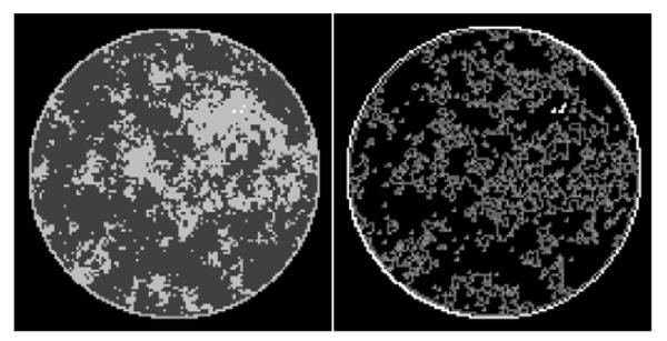
(Left) Discrete phantom modeled after a breast CT application shown in the gray-scale window [0.174 cm⁻¹, 0.253 cm⁻¹]. (Right) Gradient magnitude image (GMI) of the phantom shown in the gray scale window [0.0 cm⁻¹, 0.1 cm⁻¹]. The units of the GMI are also cm⁻¹, because the numerical implementation of ▽ involves only the differences between neighboring pixels without dividing by the physical pixel dimension. The phantom array is composed of 12,892 pixel values, and there are 4,053 non-zero values in the GMI.

A. DETERMINING ν AND λ

As shown in Eq. (17), the two linear transforms ▽ and X are combined into the transform K with the combination parameter ν. Different values of ν do not affect the solution of the optimization problems considered here, but it can affect the value of ∥K∥₂ and consequently the step length and convergence rate of the CP algorithms. If the system configuration is fixed, then it is worthwhile to perform a parameter sweep over ν to find the value which leads to the fastest convergence rate. But for our purpose, where we are varying the configuration, such a parameter study is not beneficial. It is important, however, to standardize this parameter, because altering properties of the system model can implicitly yield quite different effective values of ν. The reason for this is that the spectrum of X varies substantially depending on the size of the data vector and image array, and the physical units of projection and image gradient values are different. To standardize ν, we define:

$${\nu }_{\text{crit}}\equiv {\Vert X\Vert }_2∕{\Vert \nabla \Vert }_2.$$ (25)

The critical value of ν, ν_crit, is chosen so that ∥X∥2 equal to ν∥▽∥₂. Note that altering units on one of the transforms is automatically compensated with a different value of ν_crit. For the present investigations ν = ν_crit unless stated otherwise.

The role of λ is more important than that of ν for the reweighting algorithms, because adjusting λ both affects convergence speed and enables control over the stability of the reweighted constrained TpV minimization. In order to separate these two roles of λ, we illustrate its effect on the convex case p = 1, and a nonconvex example with p = 0.5. In the convex p = 1 case stability of the algorithm is not an issue because there is no reweighting as the weights in Algorithm 2 evaluate to unity.

For this illustration, an ideal data simulation is specified where the number of views are too few for X to have a left inverse. The number of views is set to 25, a value which will turn out to be too few for convex TV minimization, but sufficient for nonconvex TpV minimization. The simulation data are consistent in that no noise is included and the projector for the data matches that of the algorithm. Accordingly, we select ∊ = 0 for the test runs.

A Run of Constrained TV Minimization, the p = 1 Case

Figure 2 plots the various convergence metrics and the image RMSE for 1,000 iterations of Algorithm 2 with p = 1 and ∊ = 0. Note that the value of η plays no role for p = 1, because the exponent in the expression of the weights is p – 1 and accordingly the weights will all be unity in this case regardless of the value of η. Individual runs for λ = 10⁻⁴, 10⁻³, and 10⁻² are shown. We discuss the convergence criteria from top to bottom.

FIGURE 2.

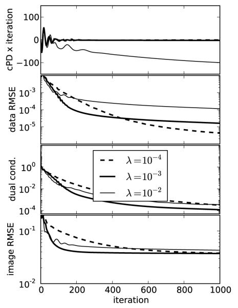
Convergence plots for image reconstruction from noiseless data containing 25 projections using Algorithm 2 with three different values of λ. For these results, we set p = 1.0 which yields convex constrained TV minimization and set ∊ = 0. The top three plots are used to evaluate convergence of the algorithm, and the middle value λ = 10⁻³ shows the fastest convergence rate. Note that for this convex case Algorithm 2 is proved to converge for any value of λ. The bottom plot indicates the discrepancy from the test phantom. The image RMSE is normalized by dividing the actual RMSE values in cm⁻¹ by 0.194 cm⁻¹, the linear attenuation coefficient of the background fat tissue. That this image RMSE does not tend to zero while the convergence criteria do results from the fact that too few projections are available for accurate reconstruction by constrained TV minimization. Another indication for having too few views is that the solution TV is less than the test phantom TV.

The top panel of Figure 2 indicates the value of cPD multiplied by the iteration number. This plot is shown this way because cPD can be either negative or positive as it approaches zero, and multiplication by the iteration number helps to indicate the empirical convergence rate of this metric for different values of λ. From this sub-figure we see that the values of λ = 10⁻⁴, and 10⁻³ show empirical convergence faster than the reciprocal of the iteration number while cPD corresponding to λ = 10⁻² shows a convergence rate near the reciprocal of the iteration number. The second panel of Figure 2 indicates the data RMSE, which tends to zero because the data are ideal. The third panel shows the constraint on the dual variables from Eq. (22) by plotting the left hand side of this equation, and this quantity also tends to zero. In each of these convergence plots we obtain the fastest rate with λ = 10⁻³, among the three values shown. The image RMSE shown in the bottom panel is not a convergence metric because it says nothing about whether or not the image estimate is a solution to Eq. (4), but this metric is clearly of theoretical interest because it is an indicator of the success of the image reconstruction. For 25 views and p = 1, we see that the image RMSE is tending to a non-zero value and that the number of views is insufficient for exact image recovery.

A Run of Constrained TpV Minimization, the p = 0.5 Case

For this p = 0.5 case all conditions are kept the same as the previous p = 1.0 case except for the p value, and we point out that the value of η = 0.194 × 10⁻² cm⁻¹ now plays a role, η here is selected to be 1% of the background fat attenuation coefficient. The corresponding convergence plots are shown in Figure 3, and similar convergence rates to the p = 1.0 case are seen with a couple of notable exceptions. First, the λ = 10⁻² case yields unstable iteration as indicated by a steady, if slow, increase in cPD and a level dependence of the data RMSE and dual constraint. Second, the convergence rates, according to the convergence criteria, seem to be similar between λ = 10⁻⁴ and 10⁻³, yet the image RMSE for λ = 10⁻³ shows much lower values and a rapid drop at 500 iterations.

FIGURE 3.

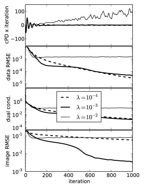
Same as Figure 2 except p = 0.5 yielding a nonconvex constrained TpV minimization problem. For p < 1, selecting λ too large can lead to unstable behavior seen in the λ = 10⁻² case as convergence metrics do not decay with iteration number. The fat normalized image RMSE plot is interesting in that the curve corresponding to λ = 10⁻³ shows a rapid drop at 500 iterations and correspondingly we see in Figure 4 that this run accurately recovers the phantom within the 1,000 iterations.

The corresponding images at iteration 1,000 along with the TV weights are shown in Figure 4. The image estimates corroborate the image RMSE plot from Figure 3 showing accurate recovery for λ = 10⁻³ alone at 1,000 iterations. We reiterate that the reason for image estimate inaccuracy is different for λ = 10⁻² and 10⁻⁴. For the former case, the reweighting is unstable and the test phantom will not be recovered at any iteration number, while for the latter case, the reweighting is stable but more iterations are needed. Indeed, for this particular case, we have continued the iteration and find that the test phantom is accurately recovered at 2,500 iterations for λ = 10⁻⁴.

FIGURE 4.

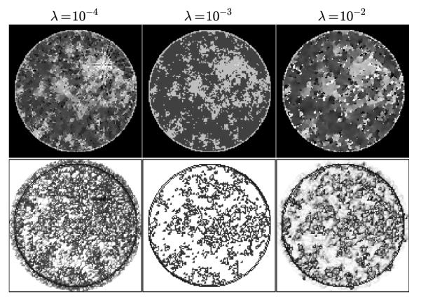
Top row shows images at iteration 1,000 obtained for various values of λ using Algorithm 2 for p = 0.5. It is clear that the phantom is recovered visually at this iteration number for λ = 10⁻³. Shown in the bottom row are the computed weighting images at iteration 1,000. For the recovered case of λ = 10⁻³ the weight image is 1.0 at all pixels where the GMI is zero.

As an aid to determining optimal values of λ, we have found it useful to monitor the change in the weighting function:

$$\Delta w={\Vert w_{n+1}-w_n\Vert }_2,$$ (26)

and partial step lengths:

$$\Delta d={\Vert X^T(y_{n+1}-y_n)\Vert }_2,$$ (27)

$$\Delta h={\Vert \nu {\nabla }^T(z_{n+1}-z_n)\Vert }_2.$$ (28)

The use of △w is straightforward as it is reasonable to expect that the weighting function should converge to a fixed weight if the reweighting procedure is stable. As seen in the top panel of Figure 5, △w decreases to the lowest value for λ = 10⁻³. For λ = 10⁻², △w does not decay, which is consistent with instability of the reweighting, and for λ = 10⁻⁴, △w does show steady decay but just not as rapid as that of λ = 10⁻³. It is also useful to examine the magnitude of the separate terms in the image update at line 12 of Algorithm 2. The quantity △d indicates the change in the image estimate due to data fidelity, and △h represents the change in the image due to the weighted TV minimization. Empirically, we find the best convergence behavior when △h is of similar magnitude to △d and λ is an effective control parameter for controlling the relative sizes of these step lengths. For the convex case of p = 1.0, we find that △h and △d are still useful for selecting λ, but clearly △w is not because there is no reweighting involved.

FIGURE 5.

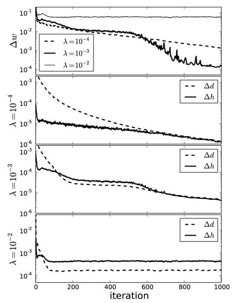
As an aid to selecting λ it is useful to plot the step lengths △d and △h, defined in the text, as a function of iteration number. If △d ⪢ △h, λ is too low yielding slow convergence. If △d ≈ △h, λ is near the optimal value for algorithm convergence rate. If △d ⪡ △h, λ is too large and the algorithm behavior is likely unstable for p < 1. The change in the weighting image, △w shown at top, is also a useful indicator for convergence of the reweighting algorithm.

V. PHANTOM RECOVERY WITH SPARSE-VIEW SAMPLING

The isolated algorithm tests for 25 view projection data indicate the possibility for accurate image reconstruction from fewer views for nonconvex TpV minimization, at p = 0.5, than convex TV minimization. In this section, we explore this possibility more thoroughly, varying the number of views and value of p. In order to perform this parameter survey there are three technical issues to address: (1) the study design and stopping rule, (2) how to obtain results for p = 2.0, and (3) how to handle the algorithm parameter λ.

Study Design

The phantom recovery study employs ideal projection data so that only the issue of sampling sufficiency comes into question. In principle, the data error parameter ∊ could be set to zero and image RMSE computed as a function of number of views and value of p. Doing so, however, causes problems in comparing results between different parameter values, because we cannot hope to solve the optimization problem with ∊ = 0 accurately. Instead, we employ the study design from Ref. [5] and choose a small but nonzero ∊. We select ∊ so that the relative data RMSE ∊’ defined

$${∊}^{\prime }\equiv \frac{∊}{\max \left(\mathbf{g}\right)\sqrt{\text{size}\left(\mathbf{g}\right)}}$$

is 10⁻⁵. During the iteration we use a stringent stopping rule and require that

$$0.999\times {10}^{-15}\le \frac{{\Vert X{\mathbf{f}}_n-\mathbf{g}\Vert }_2}{\max \left(\mathbf{g}\right)\sqrt{\text{size}\left(\mathbf{g}\right)}}\le 1.001\times {10}^{-5},$$ (29)

for 100 consecutive iterations.

Algorithm for TpV Minimization With p = 2.0

When p = 2.0, TpV becomes the standard quadratic roughness metric, and the corresponding optimization problem is

$${\mathbf{f}}^{\circ }=\underset{\mathbf{f}}{\arg \min }\left\{\frac{\lambda }{{\nu }^2}{\Vert \nu \nabla \mathbf{f}\Vert }_2^2+{\delta }_{B_2\left(∊\right)}(X\mathbf{f}-\mathbf{g})\right\},$$ (30)

where the denominator in the first term is ν² in order to make the optimization problem independent of ν. Note that both isotropic and anisotropic TpV are the same when p = 2.0. Because the objective function is quadratic, reweighting is not necessary, and there are many algorithm choices available. In Ref. [5], the Lagrangian form of Eq. (30) is solved using the conjugate gradients algorithm adjusting the Lagrange multiplier so that the desired ∊ is obtained. For this work, we derive a different instance of the CP algorithm to handle the quadratic penalty. To obtain the pseudocode, we modify Algorithm 2 by removing the reweighting, i.e. w ← 1, and replacing line 11 with

$${\overrightarrow{\mathbf{z}}}_{n+1}\leftarrow {\overrightarrow{\mathbf{z}}}_n^{\prime }∕(1+\sigma {\nu }^2∕(2\lambda \left)\right).$$

This modification directly solves the constrained quadratic roughness problem.

Automatic Setting of the Algorithm Parameter λ

As noted in Sec. IV-A, there is trial and error involved in selecting the optimal value of λ for fastest algorithm convergence. While this issue is manageable for a fixed configuration, it complicates surveys over configuration parameters, such as the number of views, because the optimal λ is likely different for each configuration. Furthermore, a bad choice of λ leading to instability of the reweighting causes the algorithm to never terminate by the specified stopping rule. In order to complete the parameter survey without intervention, we allow λ to vary with iteration number according to the following formula:

$${\lambda }_n\leftarrow {\lambda }_0{2}^{-\lfloor {\log }_{2}n\rfloor },$$ (31)

yielding the sequence

$${\lambda }_n={\lambda }_0\left\{1,\frac{1}{2},\frac{1}{2},\frac{1}{4},\frac{1}{4},\frac{1}{4},\frac{1}{4},\frac{1}{8},\dots \right\}.$$ (32)

By having a decaying schedule for λ, we are assured that at some finite iteration number the reweighting algorithm becomes stable and dwelling on fixed values yields behavior similar to the basic algorithm within the plateaus of λ_n. Opening this possibility of variable λ_n raises the question of other decay schedules or adaptive control, but such studies are beyond the scope of this article.

For the present results where p is varied in [0.1, 2.0] and the number of views range from 18 to 80, we find the sequence of λ_n in Eq. (31) sufficient. Furthermore, with λ₀ set to 1, the algorithm automatically converges to a solution satisfying the stopping rule specified in Eq. (29) for all numbers of views and values of p in the scope of the study. The smallest and largest number of iterations required are 4,331 and 33,920, respectively. Even though we found it sufficient to set λ₀ = 1, we introduce this parameter in case there are other conceivable tomographic system configurations that call for larger λ.

A. TEST PHANTOM RECOVERY RESULTS

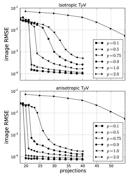
The phantom recovery results for both isotropic and anisotropic TpV minimization are summarized in Figure 6. For reference, we include the p = 2.0 case, which does not exploit GMI sparsity. The image RMSE is reported as a fraction of the background fat attenuation. In the plots the image RMSE can be small, but it cannot be numerically zero because the data error tolerance parameter ∊ is not zero. Nevertheless some parameter choices lead to small image RMSE values, and for this work we say that the image is accurately recovered if the image RMSE is less than 10⁻³, or in other words 0.1% of fat attenuation. By comparison, the contrast between fibroglandular and fat is 20%. Because image reconstruction by constrained TpV minimization exploits GMI sparsity, it is interesting to compare number of samples m = size(g) for accurate image recovery to the number of GMI nonzeros.

FIGURE 6.

Image recovery plots for both isotropic and anisotropic TpV minimization subject to the data error constraint ∊’ = 10⁻⁵. The constraint parameter on the data RMSE is related to the ℓ₂ data error tolerance by: ${∊}^{\prime }=∊∕\left(\mathbf{max}\right(\mathbf{g}\left)\sqrt{\mathit{m}}\right)$, where m = size(g) is the total number of measurements.

Accurate recovery for the p = 2.0 case, which is the same for both isotropic and anisotropic TpV, occurs at 80 views – a number which can be interpreted as full sampling for the problem. At this number of views, the number of samples is m = 20,480 which is about 67% more than the number of pixels in the image array. That such an overdetermined configuration is needed for accurate image reconstruction for p = 2 is a consequence of the condition number of X [5].

For p ≤ 1, both isotropic and anisotropic TpV minimization are exploiting GMI sparsity for accurate image reconstruction and it is clear from both graphs that substantial reduction in the number of samples is permitted by this strategy. Starting with isotropic TpV, we observe that for the convex case, p = 1, accurate image reconstruction occurs at 35 views where m = 8,960 which is less than the number of image pixels n = 12,892 and is a little more than twice the phantom GMI sparsity 4,053. Reducing p to p < 1, leads to nonconvex TpV minimization but also to more effective exploitation of GMI sparsity. As seen in the top graph of Figure 6, even introducing a little nonconvexity as in the p = 0.9 case yields a dramatic drop in the number of views as we obtain accurate image reconstruction at 30 views, where m = 7,680. For the present simulation, it appears that this strategy saturates at p = 0.5, where accurate image reconstruction occurs at 22 views and even going to p = 0.1 does not alter the necessary number of projections. Although, we do note that p = 0.1 does yield slightly smaller image RMSE than p = 0.5, indicating a possible increased robustness to some forms of data inconsistency. At 22 views, the number of samples is quite low as m = 5,632, which is only 39% greater than the number of GMI nonzeros.

Comparing anisotropic TpV with the isotropic case, we observe that even greater sampling reduction is seen as accurate image reconstruction is observed at lower numbers of views for p ≤ 1. For p = 0.1 and 0.5, accurate image reconstruction is obtained at 20 views, corresponding to m = 5,120 – only 26% greater than the number of GMI nonzeros. One might argue that the GMI sparsity might not provide the correct reference for anisotropic TpV and instead sparsity in the phantom gradient itself should be the correct quantity of comparison. But we point out that the components of the phantom gradient are not independent, and the GMI sparsity provides a better estimate of the number of underlying independent parameters for the phantom gradient.

VI. IMAGE RECONSTRUCTION WITH NOISY PROJECTION DATA

The previous sets of results demonstrate the theoretical motivation of constrained TpV minimization for image reconstruction in CT. To consider use of the above algorithms on clinical data, it is important to understand the algorithms’ response to inconsistency with the employed data model in Eq. (2). Response to data inconsistency is important to assess, because it provides a sense of algorithm robustness and because algorithm implementation choices, equivalent under ideal data conditions, may not be equivalent in the presence of data inconsistency. The data model used in the present formulation of constrained TpV minimization is simplistic in that it ignores important physical factors such as the polychromaticity of the X-ray beam, X-ray scatter, partial volume averaging, and noise. While it may be possible to include some of these physical factors into the constrained TpV minimization for the purpose of potential image quality gain, such an effort is beyond the scope of this article. Instead, in this section we present reconstructed images from simulated data including one of the most important sources of data inconsistency for the breast CT application, namely noise. Later, in Sec. VII, we present reconstructed images from an actual breast CT scan data set, which naturally includes all the physical factors implicitly.

In this section, the simulated projection data are generated from a data model where the system size is scaled up and noise is included at a level typical of breast CT. The breast CT model is challenging because the prototype systems are designed to function at very low X-ray intensities so that the exposure to the subject is equivalent to two-view full-field digital mammography [35].

The image array is taken here to be the inscribed circle of a 512 × 512 pixel array with the square pixels having width 0.35 mm. The scan configuration is again circular fan-beam with the same geometry as described in Sec. IV, but the number of projections is 200 and the detector now consists of 1024 bins of width 0.36 mm. Noise is generated using a Poisson model with mean equal to the computed mean of the number of transmitted photons at each detector bin, where the integrated incident flux at each bin, per projection, is 66,000 photons. For the present simulations, the breast phantom is also modified in order to avoid isolated pixels of fibroglandular tissue. The phantom is generated, as before, with a power law noise distribution, but this image is smoothed by a Gaussian with 4 pixel full-width-half-maximum (FWHM) prior to binning into fat and fibroglandular tissues. No microcalcifications are modeled in the phantom. The new phantom and fan-beam FBP reconstructed images are shown in Figure 7.

FIGURE 7.

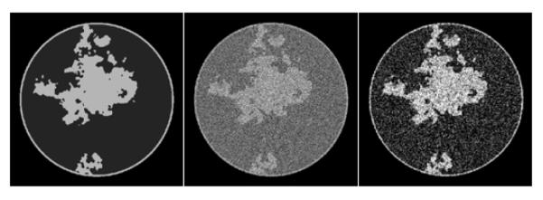
A breast CT simulation using linear attenuation coefficients for a 50 keV mono-energetic X-ray beam. The noise level is typical for prototype breast CT scanners. Shown are FBP reconstructions with a ramp filter and the same image after smoothing by a Gaussian of FWHM of 0.8 pixels. The FBP images serve to indicate visually the noise level inherent in the data.

The purpose of the present simulations is to illustrate in detail how realistic and challenging levels of data inconsistency impact the TpV motivated reweighting algorithm. The number of projections, being selected as 200, is fewer than the 500 views acquired in typical breast CT prototypes. For 200 projections the total number of samples is 200 × 1024 = 204,800, and the number of pixels is 205,892. While this system is undersampled, it is more than the number required by constrained TpV minimization for accurate image reconstruction from noiseless data at any value of p ≤ 1. In this way we isolate the issue of noise response, separating it from projection angular undersampling.

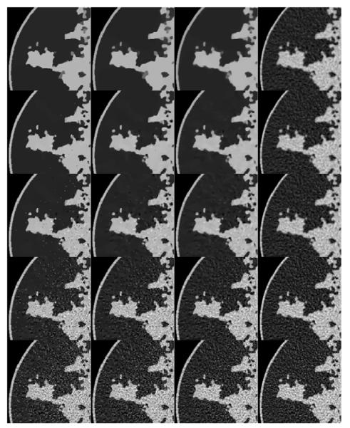
The results for image reconstruction by constrained TpV minimization for nonconvex p = 0.5 and 0.8 are compared with convex p = 1.0 and 2.0 in Figure 8. One of the convenient features of employing a hard data-error constraint is that the rows of the image array have identical data fidelity, allowing us to focus only on the impact of p. We point out that the p = 2.0 case is not GMI sparsity-exploiting, and as a consequence the corresponding images potentially suffer from both noise and undersampling artifacts.

FIGURE 8.

Reconstructed ROIs for p = 0.5, 0.8, 1.0, and 2.0 for columns 1, 2, 3, and 4, respectively. The data error constraint parameter ∊ is set so as to correspond to a data RMSE of 0.015, 0.0145, 0.014, 0.012, and 0.01 for rows 1, 2, 3, 4, and 5, respectively. Shown in the array of images are a blow up ROI of the upper left side of the image so that small details can be seen clearly.

The array of images illustrates an important feature of the use of nonconvex TpV. With the underlying object model being complex, yet piecewise constant, the TpV quasinorm reduces the speckle noise in regions of uniform attenuation coefficient relative to p = 1.0 and 2.0. In terms of image RMSE relative to the truth, the panel with the lowest error appears in the second row and second column, corresponding to p = 0.8 and ∊’ = 0.0145; we point out, however, that image RMSE is not always the most appropriate measure of image quality and that image quality evaluation should take into account the imaging task [36]. Nevertheless the noise suppressing properties of TpV shows promise and may prove useful to image analysis algorithms such as those for segmentation.

Scrutinizing the nonconvex images in Figure 8, there is a potential difficulty for the breast CT application. As ∊’ increases, the speckle noise is reduced but there also appear isolated pixels with high gray values which could potentially be mistaken for microcalcifications. In practice, these isolated peaks can be differentiated from actual structure because the latter generally involve groups of pixels. Nevertheless these specks can be distracting, and we discuss their origin and how to avoid these artifacts.

In Figure 9, we focus on the panel that corresponds to p = 0.5 and ∊’ = 0.0145. On the left most column the same ROI shown in Figure 8 is shown again along with the converged weight image w. The weight image is unity in uniform regions and small at pixels belonging to the edges of tissue structures; in this way noise in the uniform regions can be heavily smoothed away without blurring the edges. In the ROI there are a few residual specks due to data noise and we can see that these specks correspond to specks of low weighting in w and these pixels are being mistaken for edge pixels of true structure. If such specks interfere with the function of the imaging system as they would, for example, in the breast CT application, there are measures which can be taken to avoid them.

FIGURE 9.

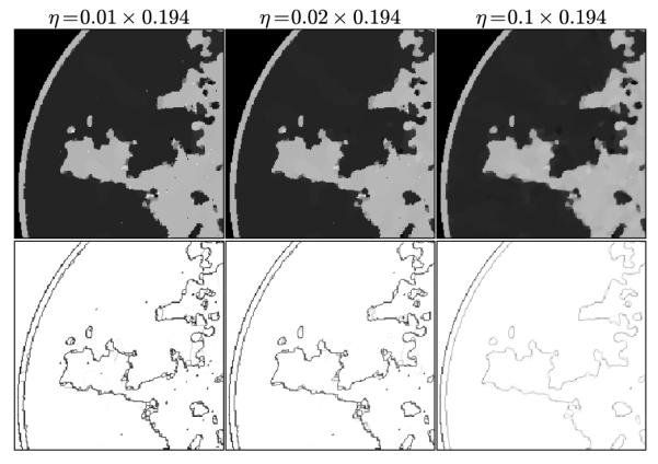
Focusing on the case of p = 0.5 and ∊ set so that the data RMSE is 0.0145, we illustrate the reconstructed ROI dependence on the parameter η in the top row. Shown in the bottom row is the corresponding impact on the weighting image.

Within the framework of the ℓ₁ reweighting algorithm, one important option is to vary η. The value of η used here is 1% of the background fat attenuation value, and it is much smaller than the contrast between fat and fibroglandular tissue. By increasing η, the speck artifacts can be removed while still maintaining some of the enhanced edge-preserving feature of the TpV reweighting scheme. The effect of increasing η is shown in the middle and right columns of Figure 9. As η increases specks are removed but the weighting at edge pixels also increases.

Another approach is to realize that the purpose of the ℓ₁ reweighting algorithm is to study image recovery under ideal data conditions, where it is important to be able to recover the phantom to arbitrarily high accuracy. For noisy data it may be advantageous to employ quadratic reweighting, which provides a different response in the image to data noise.

A. TpV MINIMIZATION BY QUADRATIC REWEIGHTING

The original nonconvex TpV minimization problem from Eq. (4) can also be addressed by use of quadratic reweighting as illustrated in Appendix VIII-A. To implement quadratic reweighting, the convex weighted ℓ₁-based optimization problem in Eq. (10) is replaced by the following convex weighted quadratic optimization problem

$${\mathbf{f}}^{\circ }=\underset{\mathbf{f}}{\arg \min }\left\{\frac{\lambda }{{\nu }^2}{\Vert \nu \sqrt{\mathbf{w}}\mid \nabla \mathbf{f}\mid \Vert }_2^2+{\delta }_{B_2\left(∊\right)}(X\mathbf{f}-\mathbf{g})\right\},$$ (33)

which modifies Eq. (30) by including a weighting factor in the quadratic roughness penalty. The corresponding dual maximization problem is

$$\begin{array}{cc}\hfill {({\mathbf{y}}^{\circ },{\overrightarrow{\mathbf{z}}}^{\circ })}^T=\underset{{(\mathbf{y},\overrightarrow{\mathbf{z}})}^T}{\arg \max }& \{-∊{\Vert \mathbf{y}\Vert }_2-{\mathbf{y}}^T\mathbf{g}-\frac{{\nu }^2}{4\lambda }{\Vert \mid \overrightarrow{\mathbf{z}}\mid ∕\sqrt{\mathbf{w}}\Vert }_2^2\phantom{\}}\hfill \\ \hfill & \phantom{\{}-{\delta }_0(-\nu {\nabla }^T\overrightarrow{\mathbf{z}}-X^T\mathbf{y})\}.\hfill \end{array}$$ (34)

and accordingly

$$\begin{array}{cc}\hfill {\mathrm{cPD}}_{\text{quad}}=& \frac{\lambda }{{\nu }^2}{\Vert \nu \sqrt{\mathbf{w}}\mid \nabla \mathbf{f}\mid \Vert }_2^2+∊{\Vert \mathbf{y}\Vert }_2+{\mathbf{y}}^T\mathbf{g}\hfill \\ \hfill & +\frac{{\nu }^2}{4\lambda }{\Vert \mid \overrightarrow{\mathbf{z}}\mid ∕\sqrt{\mathbf{w}}\Vert }_2^2.\hfill \end{array}$$ (35)

The pseudocode for TpV minimization by quadratic reweighting is given in Algorithm 4. The difference between this algorithm and Algorithm 2 appears in line 9, where the exponent of the weights expression is changed from p – 1 to p – 2, and line 11, where the form of the update step for the dual gradient variable is altered.

The quadratic reweighting algorithm has a different response to noise and other inconsistency mainly because of the parameter η. The weighted image roughness term with finite η is smooth, whereas the same term for ℓ₁-reweighting is nonsmooth even when η > 0. To see the qualitative difference between these algorithms, Figure 10 shows ROIs for these algorithms and the same parameters p = 0.8 and ∊’ = 0.0145. For both ROIs η = 0.194 × 10⁻² cm⁻¹, which is 1% of the fat attenuation. The quality of the noise is markedly different with the quadratic reweighting exchanging the sparse specks with more blobby variations which would not be mistaken for microcalcifications.

Algorithm 4.

Pseudocode for N Steps of the CP Algorithm Instance for Quadratic Reweighted Constrained TpV Minimization

1: INPUT: data g, data-error tolerance ∊, exponent p, and smoothing parameter η

2: INPUT: algorithm parameters ν; λ

3: L ← ∥(X, ν▽)∥2; τ ← 1/L; σ ← 1/L; θ ← 1; n ←  0

4: initialize f0, y0, and ${\overrightarrow{\mathbf{z}}}_0$ to zero vectors

5: ${\stackrel{‒}{\mathbf{f}}}_0\leftarrow {\mathbf{f}}_0$

6: repeat

7: ${\mathbf{y}}_n^{\prime }\leftarrow {\mathbf{y}}_n+\sigma (X{\stackrel{‒}{\mathbf{f}}}_n-\mathbf{g})$

8: ${\mathbf{y}}_{n+1}\leftarrow \max ({\Vert {\mathbf{y}}_n^{\prime }\Vert }_2-\sigma ∊,0)\frac{{\mathbf{y}}_n^{\prime }}{{\Vert {\mathbf{y}}_n^{\prime }\Vert }_2}$

9: $\mathbf{w}\leftarrow {\left(\sqrt{{\eta }^2+{\mid \nabla {\stackrel{‒}{\mathbf{f}}}_n\mid }^2}∕\eta \right)}^{p-2}$

10: ${\overrightarrow{\mathbf{z}}}_n^{\prime }={\overrightarrow{\mathbf{z}}}_n+\sigma \nu \nabla {\stackrel{‒}{\mathbf{f}}}_n$

11: ${\overrightarrow{\mathbf{z}}}_{n+1}\leftarrow {\overrightarrow{\mathbf{z}}}_n^{\prime }∕(1+\sigma {\nu }^2∕(2\mathbf{w}\lambda \left)\right)$

12: ${\mathbf{f}}_{n+1}\leftarrow {\mathbf{f}}_n-\tau (X^T{\mathbf{y}}_{n+1}+\nu {\nabla }^T{\overrightarrow{\mathbf{z}}}_{n+1})$

13: ${\stackrel{‒}{\mathbf{f}}}_{n+1}\leftarrow {\mathbf{f}}_{n+1}+\theta ({\mathbf{f}}_{n+1}-{\mathbf{f}}_n)$

14: n ← n + 1

15: until n ≥ N

16: OUTPUT: fN

17: OUTPUT: w, yN, and ${\overrightarrow{\mathbf{z}}}_N$ for evaluating cPDquad and conditions 3.

FIGURE 10.

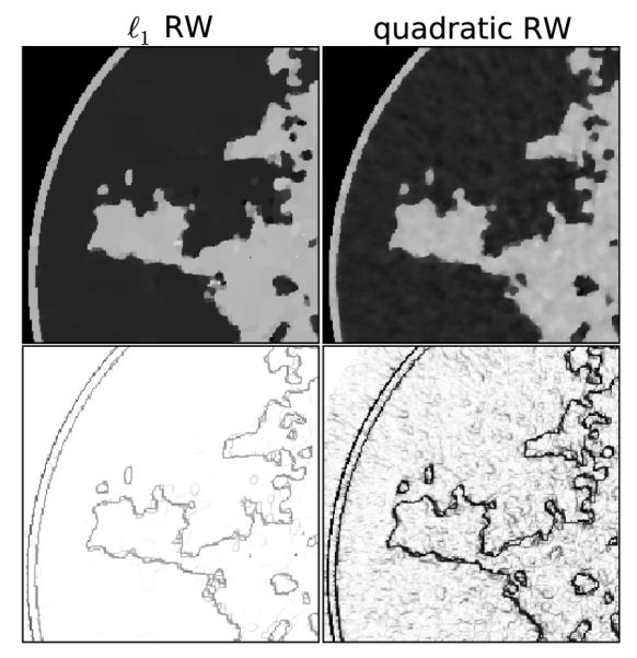
Focusing on the case of p = 0.8 and ∊’ = 0.0145, we illustrate the reconstructed ROI for (left) ℓ₁ reweighting compared with (right) quadratic reweighting. The parameter η = 0.194 × 10⁻² or 1% of the fat attenuation. Shown in the bottom row is the corresponding weighting image.

VII. APPLICATION TO CLINICAL BREAST CT DATA

While the simulations of Sec. VI illustrate the properties of the proposed IIR algorithm on a realistic simulation of breast CT, the data model used does not contain all the inconsistencies present in an actual scanner. Thus, we apply the algorithm to a clinical breast CT data set. The purpose of doing so is to first demonstrate that use of nonconvex TpV minimization can yield useful images under actual clinical conditions, and that the nonconvexity of the problem formulation does not lead to strange image artifacts. The second goal is to survey image properties for different values of p and data-error fidelity parameter ∊. To this end we perform reconstructions on a single data set, displaying the same slice. We make no attempt to find optimal p and ∊, nor to claim that the present algorithm is better than other image reconstruction algorithms. Ultimately, evaluation of the algorithm needs to be tied together with acquisition optimization. As the present algorithm appears to be robust against angular undersampling, it is possible that the breast CT acquisition could be altered to include fewer projections in a step-and-shoot mode, allowing for greater X-ray intensity for each projection, while maintaining the total dose of 2 mammographic projections.

The prototype breast CT scanner at UC Davis is described in Refs. [37] and [38]. The data set consists of 500 projection views acquired on a 768 × 1024 flat-panel detector with pixel size of (0.388 mm)². The volume reconstruction is performed on a 700×700×350 image array with cubic voxels of dimen sion (0.194 mm)³.

The particular version of TpV minimization is quadratic reweighting, shown in Algorithm 4, with η = 0.194 × 10⁻² cm⁻¹, the same value as the simulation. For quadratic reweighting, the p = 2 case does not need to be dealt with separately as is the case for ℓ₁ reweighting. Setting p = 2 in Algorithm 4 sets the weights w to one. For each reconstruction, the TpV minimization algorithm is run for 1000 iterations in order to obtain converged volumes, but we note that in practice this may be too high a computational burden and that it is likely not necessary to obtain accurate convergence for TpV minimization to yield clinically useful volumes [24].

Breast CT volumes are reconstructed for a range of parameters: 0.5 ≤ p ≤ 2.0, and relative data-error RMSE 0.011 ≤ ∊’ ≤ 0.012. For reference to the standard image reconstruction algorithm, we show one of the TpV minimization images in comparison with image reconstruction by the Feldkamp-Davis-Kress (FDK) algorithm in Figure 11. The selected TpV minimization image for the comparison is obtained for p = 0.8 and ∊’ = 0.0115. Given that the number of projections is 500, we do not expect large differences between FDK and IIR algorithms, and we observe in Figure 11 that the two images show similar structures with the TpV minimization image showing, visually, a lower noise level. That the two images have similar structure content provides a challenging check on the TpV minimization IIR algorithm.

FIGURE 11.

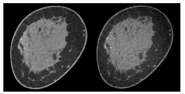
(Left) A slice from a volume reconstructed from breast CT data by TpV minimization, using quadratic reweighting. The parameters yielding this image are p = 0.8 and relative data RMSE ∊’ = 0.0115. (Right) The corresponding slice image generated by the Feldkamp-Davis-Kress (FDK) algorithm. The display gray scale window is [0.164,0.263] cm⁻¹.

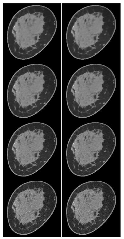
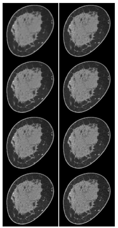
To appreciate the impact of varying p and ∊’, we show arrays of images of the same full slice in Figures 12 and 13, and ROIs in Figure 14. In the full slice images we observe little difference for the tight data-error constraint of ∊’ = 0.011, which is understandable because the view sampling rate is high and the set of feasible images satisfying the data-error constraint is relatively small. There is, however, a small but visually noticeable change in the quality of the noise as p varies. As the data-error constraint is relaxed, we observe that the smaller values of p become regularized more rapidly than larger p. The regularization for nonconvex TpV is not uniform. As ∊’ increases, noise on the soft tissue is reduced substantially while the high contrast microcalcifications are preserved with little blurring.

FIGURE 12.

Slice images obtained with TpV minimization from breast CT data for (left column) p = 0.5 and (right column) p = 0.8. The relative data-error RMSE increases from the bottom row to top row with values ∊’ = 0.011, 0.0115, 0.01175, and 0.012. The display gray scale window is [0.164,0.263] cm⁻¹.

FIGURE 13.

Same as Figure 12 except that the left and right columns show images for p = 1.0 and p = 2.0, respectively.

FIGURE 14.

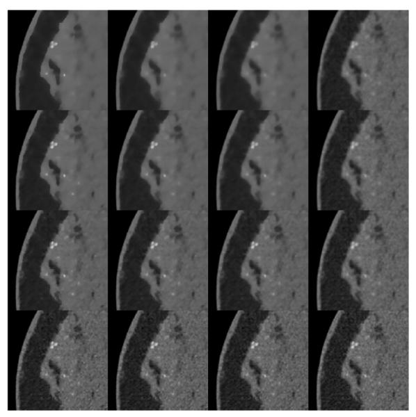
Expanded ROIs of the images shown in Figures 12 and 13. The ROI corresponds to the left-center part of the image containing the microcalcifications. The gray scale window is expanded to [0.164,0.303] cm⁻¹ in order to accommodate the higher attenuation values of the microcalcifications. The columns correspond to p = 0.5, 0.8, 1.0, and 2.0 from left to right. And the rows correspond to ∊’ = 0.011, 0.0115, 0.01175, and 0.012 from bottom to top.

To better visualize the impact of the p and ∊’ on the microcalcifications and to observe more local texture changes in the soft tissue, we show an ROI array in Figure 14. The GMI sparsity promoting values of p, p ≤ 1.0 all show rapid regularization of the soft tissue with increasing ∊’, while the texture change for p = 2.0, is much more gradual. For the higher contrast microcalcifications, the visual dependence with increasing ∊’ is quite different, depending on p. For p = 0.5, we note little change in the sharpness of the microcalcifications. Rather, the calcifications disappear as ∊’ increases with smaller calcifications disappearing at lower ∊’. At the other extreme, p = 2.0, the microcalcifications exhibit the more traditional trend of becoming more blurry, albeit that this trend is not very strong over the shown range of ∊’. The intermediate values of p show trends which are a combination of the rapid reduction in contrast and standard blurring.

With these preliminary results, we cannot yet make a recommendation for an optimal image reconstruction algorithm for the breast CT system. The results instead are intended to demonstrate the effect of the parameters p and ∊’. Moreover the proper choice of algorithm depends on the scanner configuration, visual task, and type of observer (human or machine). We do expect, however, that use of nonconvex TpV minimization will facilitate scanning configurations with a lower view angle sampling rate, which could impact the optimal balance between number of views and X-ray beam intensity.

VIII. CONCLUSION

This work develops accurate reweighting IIR algorithms for application to CT that are used to investigate sparse data image reconstruction with nonconvex TpV minimization. The algorithms are efficient enough for research purposes in that accurate solution is obtained within hundreds to thousands of iterations.

Employing ℓ₁-reweighting for both isotropic and anisotropic TpV minimization, we observe substantial reduction in the necessary number of projections for accurate recovery of the test phantom. In fact, the number of measurements needed for p = 0.5 is a small fraction larger than the number of nonzero elements of the test phantom’s GMI. These experiments do not necessarily generalize to a rule relating number of samples to GMI sparsity, but the results are nonetheless striking especially considering that the phantom has no particular symmetry and has the complexity similar to what might be found for fibroglandular tissue in breast CT. It may not be practical to reduce the number of views to the limit of ideal image recovery, but it is important to identify this limit. With this knowledge there is the option to operate at a number of views slightly greater than the recovery limit, where there are still fewer projections than what would be needed for convex TV minimization or algorithms that do not exploit GMI sparsity.

The response to noise present in a realistic breast CT simulation is also tested along with application to an actual clinical breast CT data set. The results show that the reweighting algorithms provide images that may be clinically useful. The fact that the IIR algorithms employing nonconvex TpV allows for accurate image recovery with very sparse projection data could prove interesting for fixed dose trade off studies. Namely, the operating point in the balance between number of projections and exposure per projection may be shifted toward fewer projections with the use of nonconvex TpV minimization.

Biography

EMIL Y. SIDKY (M’11) received the B.S. degree in physics, astronomy-physics, and mathematics from the University of Wisconsin - Madison in 1987 and the Ph.D. in physics from The University of Chicago in 1993. He held academic positions in physics at the University of Copenhagen and Kansas State University. He joined the University of Chicago in 2001, where he is currently a Research Associate Professor. His current interests are in CT image reconstruction, large-scale optimization, and objective assessment of image quality.

RICK CHARTRAND (M’06–SM’12) received the B.Sc. (Hons.) degree in mathematics from the University of Manitoba in 1993 and the Ph.D. degree in mathematics from the University of California, Berkeley, in 1999. He held academic positions at Middlebury College and the University of Illinois at Chicago before coming to Los Alamos National Laboratory in 2003, where he is currently a Technical Staff Member with the Applied Mathematics and Plasma Physics Group. His research interests include compressive sensing, nonconvex continuous optimization, image processing, dictionary learning, computing on accelerated platforms, and geometric modeling of high-dimensional data.

JOHN M. BOONE was born in Los Angeles, CA, USA. He received the B.A. degree in biophysics from University of California, Berkeley, in 1979 and the M.S. and Ph.D. degrees in radiological sciences from University of California Irvine in 1981 and 1985, respectively. He held faculty positions at the University of Missouri Columbia and Thomas Jefferson University, Philadelphia, PA, USA, before joining the faculty at University of California, Davis, Sacramento, CA, USA, in 1992, where he is currently a Professor and Vice Chair (Research) of radiology and Professor of biomedical engineering. His interests are in the development of dedicated breast computed tomography (CT) systems, radiation dosimetry in CT, and image quality assessment in breast imaging and body CT. He is a fellow of the American Association of Physicists in Medicine, the Society of Breast Imaging, and the American College of Radiology.

XIAOCHUAN PAN received the bachelor’s degree from Beijing University, Beijing, China, in 1982, the master’s degree from the Institute of Physics, Chinese Academy of Sciences, Beijing, in 1986, and the master’s and Ph.D. degrees from the University of Chicago, Chicago, USA, in 1988 and 1991, respectively, all in physics. He is currently a Professor with the Departments of Radiology and Radiation and Cellular Oncology and the Committee on Medical Physics, University of Chicago. His research interests include physics, algorithms, and applications of tomographic imaging. He is a recipient of awards, such as the IEEE NPSS Early Achievement Award and the IEEE EMBS Technical Award, and a fellow of AAPM, AIMBE, IAMBE, OSA, and SPIE. He has served as a chair and/or a reviewer of study sections/review panels for funding agencies, including NIH, NSF, and NSERC, as an Associate Editor (or editorial board member) for journals in the field such as the IEEE TRANSACTIONS ON MEDICAL IMAGING, IEEE TRANSACTIONS ON BIOMEDICAL ENGINEERING, IEEE JOURNAL OF TRANSLATIONAL ENGINEERING IN HEALTH AND MEDICINE, Physics in Medicine and Biology, and Medical Physics, as a Chair/Member of technical committees of professional organizations, such as IEEE and RSNA, and as a chair/member of programs, themes, and technical/scientific committees for conferences, such as IEEE EMBC, IEEE MIC, RSNA, AAPM, and MICCIA.

APPENDIX.

A. ILLUSTRATION OF REWEIGHTING FOR NONCONVEX OPTIMIZATION

For the purpose of this article being self-contained, we illustrate here a simple one dimensional example of the use of reweighting to solve a nonconvex optimization. So that there is some resemblance to the optimization problems discussed in the text, we select a constrained ℓ_p-minimization problem as an example

$$x^{\circ }=\underset{x}{\arg \min }\varphi \left(x\right)=\underset{x}{\arg \min }\{{\mid x\mid }^p+{\delta }_P(x-1\left)\right\},$$ (36)

where the set P stands for all nonnegative real numbers and the corresponding indicator function encodes the constraint x ≥ 1. The objective function of this nonconvex minimization problem is represented by the solid black curves of Figures 15 and 16.

FIGURE 15.

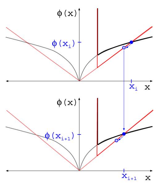
Illustration of one iteration of ℓ₁-reweighting for solving the nonconvex optimization Eq. (36). The dashed black curve is the ℓ_p quasinorm for some p with 0 < p ≤ 1. The solid black curve is the complete objective of Eq. (36). The solution estimate x_i is indicated by the solid blue circle in the top graph. The intermediate convex weighted ℓ₁ minimization is indicated by the solid red curve, where the weight is selected so that the red curve intersects the solid blue circle. The estimate x_i+1, indicated by the shaded blue circle in the top graph and the solid circle in the bottom graph, is generated by a single iteration of the Chambolle-Pock algorithm, which takes a step toward the solution. The bottom graph illustrates how the weight is adjusted so that the surrogate weighted ℓ₁ term intersects the solid blue circle corresponding x_i+1.

FIGURE 16.

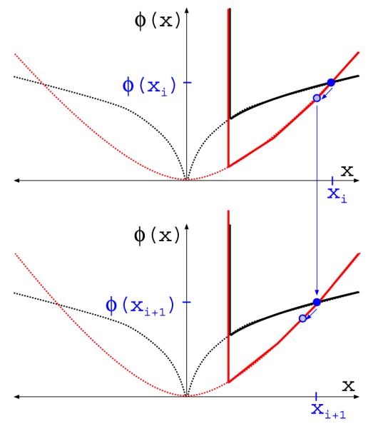
Same as Figure 15 accept that the figure illustrates quadratic reweighting.

The use of reweighting here involves making an initial estimate x_est for x. This estimate is then used to replace the nonconvex objective function with a convex function taking on the same value at x_est. In the context of ℓ₁-reweighting a weighted ℓ₁-norm replaces the ℓ_p term and the weighting factor is used to match the convex and nonconvex objectives at x_est. In this case, the weighting factor is

$$w={\mid x_{\text{est}}\mid }^p∕\mid x_{\text{est}}\mid ={\mid x_{\text{est}}\mid }^{(p-1)}.$$ (37)

The intermediate convex optimization acting as a surrogate for Eq. (36) is

$$x^{\circ }=\underset{x}{\arg \min }\varphi \left(x\right)=\underset{x}{\arg \min }\{w\mid x\mid +{\delta }_P(x-1\left)\right\},$$ (38)

which can be solved by a host of convex optimization algorithms such as the Chambolle-Pock algorithm used in the text. There is some freedom in designing the reweighting algorithm, reflecting how accurate the intermediate optimization Eq. (38) is solved. For the algorithms in the text only one iteration of the solver for the intermediate problem is taken. The result is then assigned to x_est, which is in turn used to compute new weights. An illustration of this one-intermediate-step ℓ₁-reweighting algorithm is shown in Figure 15.

For quadratic reweighting the weights and intermediate convex optimization problem are

$$w={\mid x_{\text{est}}\mid }^p∕{\mid x_{\text{est}}\mid }^2={\mid x_{\text{est}}\mid }^{(p-2)},$$ (39)

and

$$x^{\circ }=\underset{x}{\arg \min }\varphi \left(x\right)=\underset{x}{\arg \min }\left\{w{\mid x\mid }^2+{\delta }_P(x-1)\right\},$$ (40)

respectively. The corresponding one-intermediate-step quadratic reweighting algorithm is shown in Figure 16.

The 1D nonconvex problem, Eq. (36), discussed here is used for illustration purposes. But there are peculiarities of this low dimensional example. For example, it is clear from both Figures 15 and 16 that the solution of Eq. (36) coincides with the solutions of both the weighted ℓ₁ and quadratic surrogate convex optimization problems. This will not be the case for the multidimensional optimization problems considered in the text. Also, for the multidimensional case it is important to guard against potential division by zero in computing the weights. For the present one dimensional problem this danger seems remote. Nevertheless a possible corresponding weight for ℓ₁-reweighting is

$$w={\sqrt{{\eta }^2+{\mid x_{\text{est}}\mid }^2}}^{(p-1)},$$ (41)

where η is a small nonnegative real number. And similarly for quadratic reweighting

$$w={\sqrt{{\eta }^2+{\mid x_{\text{est}}\mid }^2}}^{(p-2)}.$$ (42)

The following sections show derivations for G*, F*, prox_τ [G], and prox_σ [F*] from Sec. III-A.

B. DERIVATION OF G* AND prox_τ [G]

As G(f) = 0, it is easy to show that

$$G^{\ast }\left(\mathbf{f}\right)={\delta }_0\left(\mathbf{f}\right),$$

(see for example Eq. (18) of Ref. [30] and subsequent discussion). It is also easy to show that

$${\text{prox}}_{\tau }\left[G\right]\left(\mathbf{f}\right)=\mathbf{f}.$$

C. DERIVATION OF F*

This computation is more involved, and we split this up into two, defining

$$\begin{array}{cc}\hfill F_1\left(\mathbf{y}\right)=& {\delta }_{B_2\left(∊\right)}(\mathbf{y}-\mathbf{g}),\hfill \\ \hfill F_2\left(\overrightarrow{\mathbf{z}}\right)=& \frac{\lambda }{\nu }{\Vert (\mathbf{w}\mid \overrightarrow{\mathbf{z}}\mid )\Vert }_1.\hfill \end{array}$$ (43)

Starting with $F_1^{\ast }$,

$$F_1^{\ast }\left(\mathbf{y}\right)=\underset{{\mathbf{y}}^{\prime }}{\max }\left\{{\mathbf{y}}^T{\mathbf{y}}^{\prime }-F_1\left({\mathbf{y}}^{\prime }\right)\right\}$$ (44)

$$=\underset{{\mathbf{y}}^{\prime }}{\max }\left\{{\mathbf{y}}^T{\mathbf{y}}^{\prime }-{\delta }_{B_2\left(∊\right)}({\mathbf{y}}^{\prime }-\mathbf{g})\right\};$$ (45)

substituting y” = y’ – g, we obtain

$$F_1^{\ast }\left(\mathbf{y}\right)={\mathbf{y}}^T\mathbf{g}+\underset{{\mathbf{y}}^{″}}{\max }\left\{{\mathbf{y}}^T{\mathbf{y}}^{″}-{\delta }_{B_2\left(∊\right)}\left({\mathbf{y}}^{″}\right)\right\},$$ (46)

$${\mathbf{y}}^{″}=∊\mathbf{y}∕{\Vert \mathbf{y}\Vert }_2,\text{and}$$ (47)

$$F_1^{\ast }\left(\mathbf{y}\right)={\mathbf{y}}^T\mathbf{g}+∊{\Vert \mathbf{y}\Vert }_2.$$ (48)

The maximizer, y”, at Eq. (47) is derived by noting that the objective in Eq. (46) is maximized when y” ∝ y and the magnitude of y” is limited to ∊ by the indicator function. The next term $F_2^{\ast }$ is

$$F_2^{\ast }\left(\overrightarrow{\mathbf{z}}\right)=\underset{{\overrightarrow{\mathbf{z}}}^{\prime }}{\max }\left\{{\overrightarrow{\mathbf{z}}}^T{\overrightarrow{\mathbf{z}}}^{\prime }-F_2\left({\overrightarrow{\mathbf{z}}}^{\prime }\right)\right\}$$ (49)

$$=\underset{{\overrightarrow{\mathbf{z}}}^{\prime }}{\max }\left\{{\overrightarrow{\mathbf{z}}}^T{\overrightarrow{\mathbf{z}}}^{\prime }-\frac{\lambda }{\nu }{\Vert (\mathbf{w}\mid {\overrightarrow{\mathbf{z}}}^{\prime }\mid )\Vert }_1\right\}.$$ (50)

Now we substitute the polar decompositions $\overrightarrow{\mathbf{z}}=\mathbf{z}\widehat{\mathbf{z}}$ and ${\overrightarrow{\mathbf{z}}}^{\prime }={\mathbf{z}}^{\prime }{\widehat{\mathbf{z}}}^{\prime }$, where z, z’ are non-negative scalar images and $\widehat{\mathbf{z}},{\widehat{\mathbf{z}}}^{\prime }$ are spatial unit-vector images. Since w and z are non-negative, we obtain

$$F_2^{\ast }\left(\overrightarrow{\mathbf{z}}\right)=\underset{{\mathbf{z}}^{\prime }\in {[0,\infty )}^N}{\max }\left\{{\mathbf{z}}^T{\mathbf{z}}^{\prime }-\frac{\lambda }{\nu }{\Vert \left({\mathbf{wz}}^{\prime }\right)\Vert }_1\right\}$$ (51)

$$=\underset{{\mathbf{z}}^{\prime }\in {[0,\infty )}^N}{\max }\left\{{\mathbf{z}}^T{\mathbf{z}}^{\prime }-\frac{\lambda }{\nu }{\mathbf{w}}^T{\mathbf{z}}^{\prime }\right\}$$ (52)

$$={\delta }_{E_{\infty }(\lambda \mathbf{w}∕\nu )}(\mid \overrightarrow{\mathbf{z}}\mid ).$$ (53)

In going from Eq. (50) to Eq. (51), we note that the second term in the objective does not depend on ${\widehat{\mathbf{z}}}^{\prime }$ and, fixing ${\mathbf{z}}^{\prime }$ and allowing ${\widehat{\mathbf{z}}}^{\prime }$ to vary, the objective function is maximized when the spatial-unit-vectors in ${\widehat{\mathbf{z}}}^{\prime }$ point in the same direction as $\widehat{\mathbf{z}}$, i.e. ${\widehat{\mathbf{z}}}^{\prime }=\widehat{\mathbf{z}}$. The indicator function at the last line comes about from considering two cases regarding the coefficient of z’ in Eq. (52): if all components of z – λw/ν are non-positive the objective function is maximized at z’ = 0 where its value is zero; otherwise if one component of z – λw/ν is positive the objective function can be made arbitrarily large. Equivalently, the coefficients of z/(λw/ν) can be compared to 1: if the maximum coefficient, i.e. ∥z/(λw/ν)∥_∞, is less than 1 then the maximization problem yields 0; otherwise, it yields ∞.

Combining the terms,

$$F^{\ast }(\mathbf{y},\overrightarrow{\mathbf{z}})={\mathbf{y}}^T\mathbf{g}+∊{\Vert \mathbf{y}\Vert }_2+{\delta }_{E_{\infty }(\lambda \mathbf{w}∕\nu )}(\mid \overrightarrow{\mathbf{z}}\mid ).$$ (54)

D. DERIVATION OF prox_σ [F*]$(\mathbf{y},\overrightarrow{\mathbf{z}})$

Next we compute prox_σ$\left[F_1^{\ast }\right]$(y):

$${\text{prox}}_{\sigma }\left[F_1^{\ast }\right]\left(\mathbf{y}\right)=\underset{{\mathbf{y}}^{\prime }}{\arg \min }\left\{{\mathbf{y}}^{\prime T}\mathbf{g}+∊{\Vert {\mathbf{y}}^{\prime }\Vert }_2+\frac{1}{2\sigma }{\Vert \mathbf{y}-{\mathbf{y}}^{\prime }\Vert }_2^2\right\}$$ (55)

$$=\underset{{\mathbf{y}}^{\prime }}{\arg \min }\left\{∊{\Vert {\mathbf{y}}^{\prime }\Vert }_2+\frac{1}{2\sigma }{\Vert {\mathbf{y}}^{\prime }-\mathbf{y}+\sigma \mathbf{g}\Vert }_2^2\right\},$$ (56)

by completing the square and ignoring terms independent of y’. From the symmetry of the objective function in Eq. (56), the minimizer lies on the segment between y’ = 0 and y’ = y – σg, so we can convert to a scalar minimization problem over non-negative y’ as follows:

$${\text{prox}}_{\sigma }\left[F_1^{\ast }\right]\left(\mathbf{y}\right)=\frac{\mathbf{y}-\sigma \mathbf{g}}{{\Vert \mathbf{y}-\sigma \mathbf{g}\Vert }^2}$$ (57)

$$\times \underset{y^{\prime }\in [0,\infty )}{\arg \min }\left\{∊y^{\prime }+\frac{1}{2\sigma }{(y^{\prime }-{\Vert \mathbf{y}-\sigma \mathbf{g}\Vert }_2)}^2\right\}$$ (58)

$$=\max ({\Vert \mathbf{y}-\sigma \mathbf{g}\Vert }_2-\sigma ∊,0)\frac{\mathbf{y}-\sigma \mathbf{g}}{{\Vert \mathbf{y}-\sigma \mathbf{g}\Vert }^2}.$$ (59)

Now we compute prox_σ$\left[F_2^{\ast }\right]\left(\overrightarrow{\mathbf{z}}\right)$:

$${\text{prox}}_{\sigma }\left[F_2^{\ast }\right]\left(\overrightarrow{\mathbf{z}}\right)=\underset{{\overrightarrow{\mathbf{z}}}^{\prime }}{\arg \min }\left\{{\delta }_{E_{\infty }(\lambda \mathbf{w}∕\nu )}(\mid {\overrightarrow{\mathbf{z}}}^{\prime }\mid )+\frac{1}{2\sigma }{\Vert \overrightarrow{\mathbf{z}}-{\overrightarrow{\mathbf{z}}}^{\prime }\Vert }_2^2\right\}$$ (60)

$$=\widehat{\mathbf{z}}\underset{{\mathbf{z}}^{\prime }}{\arg \min }\left\{{\delta }_{E_{\infty }(\lambda \mathbf{w}∕\nu )}\left({\mathbf{z}}^{\prime }\right)+\frac{1}{2\sigma }{\Vert \mathbf{z}-{\mathbf{z}}^{\prime }\Vert }_2^2\right\},$$ (61)

by making the same polar decomposition substitutions as in Eq. (51), because the indicator term does not depend on ${\widehat{\mathbf{z}}}^{\prime }$ and the quadratic term is minimized when ${\widehat{\mathbf{z}}}^{\prime }=\widehat{\mathbf{z}}$ for fixed ${\mathbf{z}}^{\prime }$. The objective function of Eq. (61) is separable and the result of the minimization is a component-wise thresholding of z by the maximum value of the corresponding component of λw/ν:

$${\text{prox}}_{\sigma }\left[F_2^{\ast }\right]\left(\overrightarrow{\mathbf{z}}\right)=\widehat{\mathbf{z}}\min (\lambda \mathbf{w}∕\nu ,\mathbf{z})$$ (62)

$$=\overrightarrow{\mathbf{z}}(\lambda \mathbf{w}∕\nu )∕\max (\lambda \mathbf{w}∕\nu ,\mathbf{z}).$$ (63)

The form of the prox in Eq. (63) is equivalent to that of Eq. (62), but it is computationally more convenient because the computation of $\widehat{\mathbf{z}}$ in Eq. (62) needs to avoid potential division by zero. The denominator of Eq. (63), on the other hand, is strictly positive.

REFERENCES

- [1].Sidky EY, Kao C-M, Pan X. Accurate image reconstruction from few-views and limited-angle data in divergent-beam CT. J. X-Ray Sci. Technol. 2006 Jun.14(no. 2):119–139. [Google Scholar]
- [2].Sidky EY, Pan X. Image reconstruction in circular cone-beam computed tomography by constrained, total-variation minimization. Phys. Med. Biol. 2008 Sep.53(no. 17):4777–4807. doi: 10.1088/0031-9155/53/17/021. [DOI] [PMC free article] [PubMed] [Google Scholar]
- [3].Defrise M, Vanhove C, Liu X. An algorithm for total variation regularization in high-dimensional linear problems. Inverse Problems. 2011;27(no. 6):065002-1–065002-16. [Google Scholar]
- [4].Jensen TL, Jørgensen JH, Hansen PC, Jensen SH. Implementation of an optimal first-order method for strongly convex total variation regularization. BIT Numer. Math. 2012;52(no. 2):329–356. [Google Scholar]
- [5].Jørgensen JS, Sidky EY, Pan X. Quantifying admissible undersampling for sparsity-exploiting iterative image reconstruction in X-ray CT. IEEE Trans. Med. Imag. 2013 Feb.32(no. 2):460–473. doi: 10.1109/TMI.2012.2230185. [DOI] [PMC free article] [PubMed] [Google Scholar]
- [6].Ramani S, Fessler J. A splitting-based iterative algorithm for accelerated statistical X-ray CT reconstruction. IEEE Trans. Med. Imag. 2012 Mar.31(no. 3):677–688. doi: 10.1109/TMI.2011.2175233. [DOI] [PMC free article] [PubMed] [Google Scholar]
- [7].Chen GH, Tang J, Leng S. Prior image constrained compressed sensing (PICCS): A method to accurately reconstruct dynamic CT images from highly undersampled projection data sets. Med. Phys. 2008 Feb.35(no. 2):660–663. doi: 10.1118/1.2836423. [DOI] [PMC free article] [PubMed] [Google Scholar]
- [8].Bian J, Siewerdsen JH, Han X, Sidky EY, Prince JL, Pelizzari CA, et al. Evaluation of sparse-view reconstruction from flat-panel-detector cone-beam CT. Phys. Med. Biol. 2010 Nov.55(no. 22):6575–6599. doi: 10.1088/0031-9155/55/22/001. [DOI] [PMC free article] [PubMed] [Google Scholar]
- [9].Sidky EY, Anastasio MA, Pan X. Image reconstruction exploiting object sparsity in boundary-enhanced X-ray phase-contrast tomography. Opt. Exp. 2010 May;18(no. 10):10404–10422. doi: 10.1364/OE.18.010404. [DOI] [PMC free article] [PubMed] [Google Scholar]
- [10].Ritschl L, Bergner F, Fleischmann C, Kachelrieß M. Improved total variation-based CT image reconstruction applied to clinical data. Phys. Med. Biol. 2011 Mar.56(no. 6):1545–1562. doi: 10.1088/0031-9155/56/6/003. [DOI] [PubMed] [Google Scholar]
- [11].Han X, Bian J, Eaker DR, Kline TL, Sidky EY, Ritman EL, et al. Algorithm-enabled low-dose micro-CT imaging. IEEE Trans. Med. Imag. 2011 Mar.30(no. 3):606–620. doi: 10.1109/TMI.2010.2089695. [DOI] [PMC free article] [PubMed] [Google Scholar]
- [12].Han X, Bian J, Ritman EL, Sidky EY, Pan X. Optimization-based reconstruction of sparse images from few-view projections. Phys. Med. Biol. 2012 Aug.57(no. 16):5245–5274. doi: 10.1088/0031-9155/57/16/5245. [DOI] [PMC free article] [PubMed] [Google Scholar]
- [13].Song J, Liu QH, Johnson GA, Badea CT. Sparseness prior based iterative image reconstruction for retrospectively gated cardiac micro-CT. Med. Phys. 2007 Oct.34:4476–4483. doi: 10.1118/1.2795830. [DOI] [PMC free article] [PubMed] [Google Scholar]
- [14].Chen G-H, Tang J, Hsieh J. Temporal resolution improvement using PICCS in MDCT cardiac imaging. Med. Phys. 2009 Jun.36(no. 6):2130–2135. doi: 10.1118/1.3130018. [DOI] [PMC free article] [PubMed] [Google Scholar]
- [15].Bergner F, Berkus T, Oelhafen M, Kunz P, Pan T, Grimmer R, et al. An investigation of 4D cone-beam CT algorithms for slowly rotating scanners. Med. Phys. 2010 Sep.37(no. 9):5044–5054. doi: 10.1118/1.3480986. [DOI] [PubMed] [Google Scholar]
- [16].Ritschl L, Sawall S, Knaup M, Hess A, Kachelrieß M. Iterative 4D cardiac micro-CT image reconstruction using an adaptive spatio-temporal sparsity prior. Phys. Med. Biol. 2012 Mar.57(no. 6):1517–1526. doi: 10.1088/0031-9155/57/6/1517. [DOI] [PubMed] [Google Scholar]
- [17].Kuntz J, Flach B, Kueres R, Semmler W, Kachelrieß M, Bartling S. Constrained reconstructions for 4D intervention guidance. Phys. Med. Biol. 2013 May;58(no. 10):3283–3300. doi: 10.1088/0031-9155/58/10/3283. [DOI] [PubMed] [Google Scholar]
- [18].Chartrand R, Staneva V. Restricted isometry properties and nonconvex compressive sensing. Inverse Problems. 2008 Jun.24(no. 3):035020-1–035020-14. [Google Scholar]
- [19].Daubechies I, DeVore R, Fornasier M, Güntürk CS. Iteratively reweighted least squares minimization for sparse recovery. Commun. Pure Appl. Math. 2010 Jan.63(no. 1):1–38. [Google Scholar]
- [20].Chartrand R. Nonconvex splitting for regularized low-rank + sparse decomposition. IEEE Trans. Signal Process. 2012 Nov.60(no. 11):5810–5819. [Google Scholar]
- [21].Chartrand R. Nonconvex compressive sensing and reconstruction of gradient-sparse images: Random vs. tomographic Fourier sampling. Proc. IEEE ICIP. 2008 Oct.:2624–2627. [Google Scholar]
- [22].Ramirez-Giraldo JC, Trzasko J, Leng S, Yu L, Manduca A, McCollough CH. Nonconvex prior image constrained compressed sensing (NCPICCS): Theory and simulations on perfusion CT. Med. Phys. 2011 Apr.38(no. 4):2157–2167. doi: 10.1118/1.3560878. [DOI] [PMC free article] [PubMed] [Google Scholar]
- [23].Zhang X, Xing L. Sequentially reweighted TV minimization for CT metal artifact reduction. Med. Phys. 2013 Jul.40(no. 7):071907-1–071907-12. doi: 10.1118/1.4811129. [DOI] [PMC free article] [PubMed] [Google Scholar]
- [24].Sidky EY, Pan X, Reiser IS, Nishikawa RM, Moore RH, Kopans DB. Enhanced imaging of microcalcifications in digital breast tomosynthesis through improved image-reconstruction algorithms. Med. Phys. 2009 Nov.36(no. 11):4920–4932. doi: 10.1118/1.3232211. [DOI] [PMC free article] [PubMed] [Google Scholar]
- [25].Candès EJ, Romberg J, Tao T. Robust uncertainty principles: Exact signal reconstruction from highly incomplete frequency information. IEEE Trans. Inf. Theory. 2006 Feb.52(no. 2):489–509. [Google Scholar]
- [26].Candès EJ, Wakin MB. An introduction to compressive sampling. IEEE Signal Process. Mag. 2008 Mar.25(no. 2):21–30. [Google Scholar]
- [27].Chartrand R. Exact reconstructions of sparse signals via nonconvex minimization. IEEE Signal Process. Lett. 2007 Oct.14(no. 10):707–710. [Google Scholar]
- [28].Sidky EY, Chartrand R, Pan X. Image reconstruction from few views by non-convex optimization. Proc. IEEE NSS Conf. Rec. 2007 Nov.:3526–3530. [Google Scholar]
- [29].Chambolle A, Pock T. A first-order primal-dual algorithm for convex problems with applications to imaging. J. Math. Imag. Vis. 2011 May;40(no. 1):120–145. [Google Scholar]
- [30].Sidky EY, Jørgensen JH, Pan X. Convex optimization problem prototyping for image reconstruction in computed tomography with the Chambolle–Pock algorithm. Phys. Med. Biol. 2012;57(no. 10):3065–3091. doi: 10.1088/0031-9155/57/10/3065. [DOI] [PMC free article] [PubMed] [Google Scholar]
- [31].Candès EJ, Wakin MB, Boyd SP. Enhancing sparsity by reweighted ℓ1 minimization. Fourier Anal. Appl. 2008 Dec.14(no. 5):877–905. [Google Scholar]
- [32].Chartrand R, Yin W. Iteratively reweighted algorithms for compressive sensing. Proc. IEEE Int. Conf. Acoust., Speech, Signal Process. 2008 Apr.:3869–3872. [Google Scholar]
- [33].Niu T, Zhu L. Accelerated barrier optimization compressed sensing (ABOCS) reconstruction for cone-beam CT: Phantom studies. Med. Phys. 2012 Jul.39(no. 7):4588–4598. doi: 10.1118/1.4729837. [DOI] [PMC free article] [PubMed] [Google Scholar]
- [34].Reiser I, Nishikawa RM. Task-based assessment of breast tomosynthesis: Effect of acquisition parameters and quantum noise. Med. Phys. 2010 Apr.37(no. 4):1591–1600. doi: 10.1118/1.3357288. [DOI] [PMC free article] [PubMed] [Google Scholar]
- [35].Boone JM, Kwan ALC, Seibert JA, Shah N, Lindfors KK, Nelson TR. Technique factors and their relationship to radiation dose in pendant geometry breast CT. Med. Phys. 2005 Dec.32(no. 12):3767–3776. doi: 10.1118/1.2128126. [DOI] [PubMed] [Google Scholar]
- [36].Barrett HH, Myers KJ. Foundations of Image Science. Wiley; Hoboken, NJ, USA: 2004. [Google Scholar]
- [37].Kwan ALC, Boone JM, Yang K, Huang S-Y. Evaluation of the spatial resolution characteristics of a cone-beam breast CT scanner. Med. Phys. 2007 Jan.34(no. 1):275–281. doi: 10.1118/1.2400830. [DOI] [PubMed] [Google Scholar]
- [38].Prionas ND, Lindfors KK, Ray S, Huang S-Y, Beckett LA, Monsky WL, et al. Contrast-enhanced dedicated breast CT: Initial clinical experience. Radiology. 2010 Sep.256(no. 3):714–723. doi: 10.1148/radiol.10092311. [DOI] [PMC free article] [PubMed] [Google Scholar]