Automated Volumetry and Regional Thickness Analysis of Hippocampal Subfields and Medial Temporal Cortical Structures in Mild Cognitive Impairment

Abstract

We evaluate a fully automatic technique for labeling hippocampal subfields and cortical subregions in the medial temporal lobe (MTL) in in vivo 3 Tesla MRI. The method performs segmentation on a T2-weighted MRI scan with 0.4 × 0.4 × 2.0 mm³ resolution, partial brain coverage, and oblique orientation. Hippocampal subfields, entorhinal cortex, and perirhinal cortex are labeled using a pipeline that combines multi-atlas label fusion and learning-based error correction. In contrast to earlier work on automatic subfield segmentation in T2-weighted MRI (Yushkevich et al., 2010), our approach requires no manual initialization, labels hippocampal subfields over a greater anterior-posterior extent, and labels the perirhinal cortex, which is further subdivided into Brodmann areas 35 and 36. The accuracy of the automatic segmentation relative to manual segmentation is measured using cross-validation in 29 subjects from a study of amnestic Mild Cognitive Impairment (aMCI), and is highest for the dentate gyrus (Dice coefficient is 0.823), CA1 (0.803), perirhinal cortex (0.797) and entorhinal cortex (0.786) labels. A larger cohort of 83 subjects is used to examine the effects of aMCI in the hippocampal region using both subfield volume and regional subfield thickness maps. Most significant differences between aMCI and healthy aging are observed bilaterally in the CA1 subfield and in the left Brodmann area 35. Thickness analysis results are consistent with volumetry, but provide additional regional specificity and suggest non-uniformity in the effects of aMCI on hippocampal subfields and MTL cortical subregions.

1. Introduction

There has been increased interest in the recent literature in imaging the subfields of the hippocampal formation using MRI. Greater focus on subfields is driven, in part, by the desire to better characterize the complex brain networks that involve the hippocampus, and to more effectively detect the presence and progression of brain disorders to which the hippocampal region is particularly vulnerable, such as Alzheimer’s disease (AD), semantic dementia, temporal lobe epilepsy, and others. In most applications, interest is not restricted to the hippocampus alone and extends to imaging and quantification of the functionally related cortical subregions, particularly the entorhinal cortex (ERC), perirhinal cortex (PRC) and parahippocampal cortex (PHC), which together form the parahippocampal gyrus (PHG). These cortical regions are tightly interconnected with the hippocampus as part of the medial temporal memory networks (Squire et al., 2004; van Strien et al., 2009; Yassa and Stark, 2011; Wolk et al., 2011; Ranganath and Ritchey, 2013). While the cortical MTL regions appear to support episodic memory function in conjunction with the hippocampus, a number of memory models suggest dissociable representations and processes linked to these subregions (Yonelinas et al., 2010; Eichenbaum et al., 2007; Norman, 2010). For example, one particularly influential model has suggested that PRC supports object representations while the PHC supports contextual aspects of prior experience, particularly spatial. The hippocampus then binds this information together to represent rich, episodic information (Eichenbaum et al., 2007). An additional motivation for more granular measurement of MTL cortical subregions is that the PRC and ERC are amongst the earliest sites of neurodegeneration in AD (Braak and Braak, 1995; Bobinski et al., 1997; Simić et al., 1997; West et al., 2004). Similarly, hippocampal subfields are variably affected by AD pathology and also may differentially support critical memory processes, such as pattern separation and pattern completion (Yassa and Stark, 2011). Whereas hippocampal volumetry and morphometry are well-established techniques in quantitative neuroimaging, obtaining such measures at the level of hippocampal subfields and subregions of the parahippocampal gyrus has proven to be a greater technological challenge due to their small size, complex shape, and considerable anatomical variability.

Prior work on quantitative in vivo imaging of hippocampal subfields can be categorized in terms of MRI acquisition. Although MRI parameters vary widely in the subfield literature, two broad categories can be defined. In one category, there are the approaches that operate on what we will refer to as “routine” T1-weighted 1.5 or 3 Tesla MRI scans, with resolution on the order of 1 × 1 × 1 mm³ and whole-brain field of view. Such scans are acquired almost universally in today’s neuroimaging studies. In the other category are the approaches that require more “dedicated” MRI scans that target the hippocampal region specifically. An example of the “routine” and “dedicated” scans in the same subject is given in Figure 1.

Figure 1.

Example slices from the T1-weighted (left) and T2-weighted (right) images of the hippocampal region from one of the subjects in this study. The bottom panel is a zoomed in region around the right hippocampus. The T1-weighed image is representative of what we describe as “routine” MRI in the text, while the T2-weighted image is an example of a “dedicated” MRI scan tailored for hippocampal subfield imaging. The slice plane is coronal for the T1-weighted image and oblique coronal (orthogonal to the hippocampal main axis) for the T2-weighted image.

The appearance of the hippocampus in the “routine” T1-weighted scans tends to be nearly homogeneous, making it difficult to see anatomical details, such as the laminar organization of the hippocampus, that are necessary for manually labeling subfields. In fact, we are not aware of any published study that has implemented and validated a manual hippocampal subfield segmentation protocol in the “routine” T1-weighted scans. Instead, most subfield imaging work in the “routine” scans relies on computational morphological techniques. These include template-based approaches (Wang et al., 2006; Apostolova et al., 2006; Bakker et al., 2008; Yushkevich et al., 2009), which segment the hippocampus as a single structure, deform the segmented hippocampi to a volumetric or surface template, and associate regional statistics (e.g., group differences in thickness, or differences in task-related fMRI activation) with specific subfields by defining anatomical regions of interest directly in template space. A more recent class of papers uses the automatic segmentation algorithm provided by the FreeSurfer software (Van Leemput et al., 2009; Fischl, 2012; Iglesias et al., 2013) to estimate hippocampal subfield volumes directly in the “routine” T1-weighted scans. The underlying technique was developed and validated in what we would term “dedicated” T1-weighted MRI scans with 0.4 × 0.4 × 0.8mm³ resolution and acquisition time of 35 min (Van Leemput et al., 2009). However nearly all published applications of this technique have been to T1-weighted MRI with “routine” resolution on the order of 1 × 1 × 1 mm³ (e.g., Hanseeuw et al., 2011; Engvig et al., 2012; Teicher et al., 2012; Lim et al., 2012; Iglesias et al., 2013; Pereira et al., 2013). To our knowledge, the accuracy of the Van Leemput et al. (2009) technique relative to manual segmentation has not been evaluated at this lower resolution.

The “dedicated” MRI sequences targeting the hippocampus tend to have high resolution in the plane orthogonal to the hippocampal main axis (usually < 0.5 × 0.5mm²), attained at the cost of increased slice thickness, greater acquisition time, or higher MRI field strength (Zeineh et al., 2003; Mueller et al., 2007a; Mueller and Weiner, 2009; Van Leemput et al., 2009; Ekstrom et al., 2009; La Joie et al., 2013; Malykhin et al., 2010; Kerchner et al., 2010; Yassa et al., 2010; Henry et al., 2011; Bonnici et al., 2012; Wisse et al., 2012; Pluta et al., 2012; Winterburn et al., 2013; Olsen et al., 2013; Kirov et al., 2013). The majority of the “dedicated” sequences in the literature employ T2 or T2* weighting and a field of view that covers only a portion of the brain. In most subjects, such scans reveal a thin hypointense band formed by the inner lamina of the CA subfield (stratum radiatum and stratum lacunosomoleculare), the outer lamina of the dentate gyrus (DG), and the vestigial hippocampal sulcus that separates them. Abbreviated as SRLM-HS, this hypointense band can serve as a visual cue for subfield labeling. At 7 Tesla, the ability to distinguish subfield layers improves further (Thomas et al., 2008; Breyer et al., 2010; Kerchner et al., 2010; Cho et al., 2010; Prudent et al., 2010; Henry et al., 2011; Wisse et al., 2012; Kirov et al., 2013), making it possible to isolate specific strata within hippocampal subfields (Kerchner et al., 2010; Kirov et al., 2013). A number of manual segmentation protocols for “dedicated” MRI have been implemented in the literature (Mueller and Weiner, 2009; Malykhin et al., 2010; Ekstrom et al., 2009; La Joie et al., 2010; Kerchner et al., 2010; Preston et al., 2010; Libby et al., 2012; Pluta et al., 2012; Wisse et al., 2012; Olsen et al., 2013; Winterburn et al., 2013). However, there has been limited work on automatic subfield segmentation in these “dedicated” T2-weighted MRI scans (Flores, 2012; Pipitone et al., 2014). Given that manual segmentation is very time consuming, requires extensive training and evaluation, and can be subject to rater bias, there is a pressing need for an effective automatic segmentation method.

In (Yushkevich et al., 2010), we presented an automated subfield segmentation technique targeting “dedicated” T2-weighted oblique coronal MRI of the hippocampal region, and showed that the agreement between the automatic segmentation and manual segmentation was comparable to the inter-rater reliability of manual segmentation. However, our prior work had a significant limitation: the subfields were labeled only on a few MRI slices in the body region of the hippocampus. This restriction caused more than two thirds of the hippocampal formation to be ignored by the subfield measurements, which may weaken the sensitivity of the subfield measurements to hippocampal neurodegeneration, as the reduction in size along the main axis of the hippocampus is not reflected by the measurements. Restricting the segmentation to the hippocampal body also required the user to manually tag slices as belonging to the body, head or tail region, rendering the method not fully automatic. The present paper addresses these limitations by extending subfield segmentation to the whole length of the hippocampus. It also expands the number and extent of cortical subregions that are labeled, including the PRC, which is further subdivided into Brodmann areas 35 and 36.

Our approach, which we call ASHS (automatic segmentation of hippocampal subfields), leverages multi-atlas segmentation and machine learning techniques. As illustrated in Figure 2, ASHS consists of a training pipeline and a segmentation pipeline. The ASHS training pipeline takes as its input manually labeled “dedicated” T2-weighted MRI scans and whole-brain “routine” T1-weighted scans from a set of subjects and generates a dataset called an atlas package. The ASHS segmentation pipeline uses this atlas package to label T2-weighted MRI scans of new subjects automatically. In the current paper we train and evaluate ASHS using a specific T2-weighted MRI sequence and a specific manual segmentation protocol. However, the structure of ASHS allows it to be easily re-trained use data acquired with a different MRI sequence and labeled with a different segmentation protocol. Given the large variability in the imaging protocols and subfield labeling schemes proposed in the MRI literature, we view this inherent adaptability as an important strength of ASHS. An open-source implementation of ASHS is provided.¹

Figure 2.

Graphical illustration of the training and segmentation pipelines in ASHS. The ASHS training pipeline takes as its input a set of “atlas” datasets, each consisting of a T1-weighted and T2-weighted MRI scans of the same subject, and a manual segmentation of the T2-weighted MRI scan. The training pipeline outputs an “atlas package,” which is then used as the input to the ASHS segmentation pipeline. The segmentation pipeline uses the atlas package to automatically label the T2-weighted MRI of a new subject, using that subject’s T1-weighted MRI as an additional input. The steps listed in the ASHS training pipeline, as well as the composition of the atlas package, are described in Section 2.7 and further detailed in Appendix A. The steps of the ASHS segmentation pipeline are described in Section 2.8 and Appendix B.

In addition to extending the earlier segmentation approach to more slices and structures, we present a technique for regional thickness analysis of the substructures labeled by ASHS. Inspired by the hippocampus unfolding work by Zeineh et al. (2003) and Ekstrom et al. (2009), we use a smooth surface representation to model the strip of gray matter formed by the CA subfields, subiculum, ERC and PRC in each subject, and extract maps of pointwise thickness, which are then analyzed statistically in the space of an unbiased population template. Such thickness analysis provides greater regional specificity than volumetry, and can also mitigate the uncertainty of anatomical boundaries that is inherent in any volumetric subfield analysis based on in vivo MRI.

This paper evaluates ASHS in the context of amnestic Mild Cognitive Impairment (aMCI), a population enriched in patients with prodromal AD. First, cross-validation analysis is carried out on a set of 29 manually labeled MRI scans from a study of aMCI (Section 3). Second, the ability of subfield volume features derived from ASHS to discriminate between aMCI and normal controls is evaluated, compared to the discriminative ability of whole-hippocampus and subfield-specific measures extracted from T1-weighted MRI (Section 4). Lastly, regional thickness analysis is carried out on the ASHS segmentations to further localize aMCI effects in the hippocampal region (Section 5).

2. Materials and Methods

2.1. Subjects

MRI were acquired in 92 participants from a research study of aging and cognitive impairment conducted at the Penn Memory Center at the University of Pennsylvania. The subjects include 45 patients with diagnosis of aMCI (established using the Petersen (2004) criteria) and 47 cognitively normal controls recruited from the community. All subjects were recruited from the Penn Memory Center/Alzheimer’s Disease Center (PMC/ADC). The human subjects research in this study was performed in compliance with the Code of Ethics of the World Medical Association (Declaration of Helsinki) and the standards established by the University of Pennsylvania Institutional Review Board and the National Institutes of Health. All subjects provided informed consent for this study.

2.2. Image Acquisition

MRI scans were acquired on a 3T Siemens Trio scanner at the Hospital of the University of Pennsylvania over the course of 3.5 years. Most of the scans (n=77, 40 NC, 37 MCI) were acquired using an 8-channel array coil. Approximately 2.75 years into the study, the MRI protocol was changed, and scans began to be acquired using a 32-channel coil (n=15, 7 NC, 8 MCI). Both protocols include a “routine” T1-weighted (MPRAGE) whole-brain scan and a “dedicated” T2-weighted (TSE) scan with partial brain coverage and an oblique coronal slice orientation (positioned orthogonally to the main axis of the hippocampus), adapted from (Mueller et al., 2007b; Thomas et al., 2004; Vita et al., 2003). The parameters of the T2-weighted scan with the 8-channel coil are {TR/TE: 5310/68 ms, echo train length 15, 18.3 ms echo spacing, 150° flip angle, 0% phase oversampling, 0.4 x 0.4 mm² in plane resolution, 2 mm slice thickness, 30 interleaved slices with 0.6 mm gap, acquisition time 7:12 min}; with the 32-channel coil, the parameters are {TR/TE: 7200/76 ms, echo train length 15, 15.2 ms echo spacing, 150° flip angle, 75% phase oversampling, 0.4 x 0.4 mm² in plane resolution, 2 mm slice thickness, 30 interleaved slices with no gap, acquisition time 6:29 min}. The parameters of the T1-weighted scan on the 8-channel coil are {TR/TE/TI=1600/3.87/950 ms, 15° flip angle, 1.0 × 1.0 × 1.0mm³ resolution, acquisition time 5:13 min}; for the 32-channel coil, the parameters are {TR/TE/TI=1900/2.89/900 ms, 9° flip angle, 1.0 × 1.0 × 1.0 mm³ resolution, acquisition time 4:26 min}.

2.3. Image Quality Assessment

The oblique coronal T2-weighted MRI sequence used in this work is susceptible to subject motion, which can cause severe blurring of the images. As we discuss in Section 6.4, this is one of the disadvantages of “dedicated” T2-weighted subfield imaging, relative to “routine” T1-weighted MRI. Images were examined visually for the presence of artifacts, and those with severe or moderate artifact were excluded from subsequent analysis. Images with incorrectly placed field of view that fail to cover the full anterior-posterior extent of the hippocampus were also excluded. Overall, 5 of the 92 images were excluded due to motion artifact and one was excluded due to partial field of view.

2.4. Manual Segmentation

Author JP performed manual segmentation of the hippocampal subfields and the anterior subregions of the parahippocampal gyrus in T2-weighted scans of 29 subjects (15 controls, 14 aMCI). We refer to these 29 subjects as the “atlas subset”. These subjects were selected early in the study on the basis of JP’s judgment that their manual segmentation would be feasible. Due to this selection process, the image quality of the scans in the atlas set is higher than in the full dataset. All images in the atlas set were acquired using the eight-channel MRI coil.

A segmentation protocol was developed with the realization that in vivo T2-weighted MRI only offers limited visual features for differentiating between hippocampal subfields and parahippocampal gyrus subregions. Like earlier in vivo subfield segmentation protocols (Mueller and Weiner, 2009; Malykhin et al., 2010; Ekstrom et al., 2009; La Joie et al., 2010; Kerchner et al., 2010; Preston et al., 2010; Libby et al., 2012; Pluta et al., 2012; Wisse et al., 2012; Olsen et al., 2013; Winterburn et al., 2013), it relies on the combination of intensity features and geometrical rules to specify subfield boundaries. The document outlining the segmentation protocol is included as Supplementary Material. The set of anatomical labels used in the segmentation is described briefly in Table 1. For the subfields of the hippocampus, the protocol used in our previous study (Yushkevich et al., 2010) was extended to include anterior and posterior portions of the hippocampus that were previously assigned summary ‘head’ or ‘tail’ labels. This extension was informed by the use of printed atlases (Duvernoy, 2005) as well as by visual examination of postmortem MRI and histology images from (Adler et al., 2013).

Table 1.

Summary of the anatomical labels used in the manual segmentation protocol. Details of the segmentation protocol are provided in the Supplementary Material. The top portion of the table lists the “primary” labels, i.e., those assigned to voxels by manual segmentation. The bottom portion lists derived “compound” labels, which are only used in the analysis. Compound labels are derived by merging groups of primary labels (e.g., CA merges labels CA1, CA2 and CA3).

Abbr.	Name	Comments
Primary Labels
CA1 CA2 CA3	Cornu Ammonis Fields CA1-3	CA labels include stratum pyramidale and stratum oriens. The hypointense layer of voxels (understood to combine the CA strata radiatum, lacunosum and moleculare (SRLM); the vestigial hippocampal sulcus (HS); and stratum moleculare of the DG) is split evenly between the CA and DG labels. The CA2 and CA3 subfields are labeled in the posterior portion of the hippocampal head and in the body; elsewhere they are merged into the CA1 label.
DG	Dentate Gyrus	Includes the inner half of the hypointense band; the polymorphic and granular cell layers; and the hilus, which some authors consider to be CA4. (Lorente de Nó, 1934; Duvernoy, 2005)
SUB	Subiculum	Includes subiculum proper, presubiculum and parasubiculum. SUB is labeled in the head and body, but not in the tail of the hippocampus.
MISC	Miscellaneous	Used to label cysts and cerebrospinal fluid in the hippocampus.
ERC	Entorhinal cortex	The ehMTL structures are labeled beginning at the most anterior slice of the hippocampal body and ending one slice past the most anterior slice of the hippocampal head.
BA35	Brodmann area 35
BA36	Brodmann area 36
CS	Collateral Sulcus
Compound Labels (only used for analysis)
CA	Cornu Ammonis	Combines labels CA1, CA2, and CA3
HIPP	Hippocampus	Combines labels CA, DG, and SUB
PRC	Perirhinal Cortex	Combines labels BA35 and BA36

In the parahippocampal gyrus, the segmentation protocol includes the ERC and the PRC subregions, with the PRC further divided into Brodmann areas 35 and 36 (BA36/BA36). The PHC, which forms the posterior portion of the parahippocampal gyrus, was not labeled and will be included in future work. The protocol for labeling the ERC and PRC was derived from (Ding and Van Hoesen, 2010). Author SLD served as the consultant for the segmentation effort, and provided detailed feedback on the segmentation of the ERC and PRC regions in each of the atlas datasets.

2.4.1. Extent of the Subfields in the MRI Slice Direction

Although the T2-weighted MRI offers excellent resolution in the oblique coronal plane, the relatively thick slices and highly anisotropic voxels pose a challenge when defining the anterior and posterior extents of certain structures. Because the resolution along the anterior-posterior axis is low, slice boundaries are used to define the extents of several structures. The relative extent of the different labels along the T2-weighted MRI slice direction is illustrated in Figure 1. We first designate MRI slices as being in the hippocampal head, body or tail. The most posterior head slice is the slice in which the uncus first appears. The division between body and tail is defined on the basis of shape, but frequently coincides with the appearance of the wing of the ambient cistern (see Supplementary Material). Whereas the division into CA and DG labels is carried out along the entire length of the hippocampus, subfields CA2 and CA3 are only traced in the posterior portion of the head and in the body, and are merged into the CA1 label elsewhere. The subiculum (SUB) is traced in the head and body, but not in the tail. ERC, PRC and the collateral sulcus are traced in the slices beginning one slice anterior of the head, and ending one slice posterior of the head. It is important to note that these slice boundaries are somewhat artificial, and that the actual structures extend beyond the designated slice boundaries. The need to impose these boundaries is one of the main limitations of the anisotropic T2-weighted MRI modality.

2.4.2. Intra-Rater Reliability Analysis

Approximately five months after the completion of the segmentation of the atlas set, a subset of the subjects in the atlas set (“reliability” subset) were randomly chosen and re-segmented by rater JP to compute intra-rater reliability. The reliability subset includes data from 12 subjects (6 aMCI, 6 NC). The structures in the left hemisphere were selected in half of the subjects (N=6, 3 aMCI and 3 NC), and in the other half, the right hemisphere was segmented.

2.5. Overview of ASHS Algorithm and Software

The open-source ASHS software implementation consists of shell scripts that invoke image analysis algorithms from publicly available software packages FSL (Smith et al., 2004) and ANTS (Avants et al., 2008a). ASHS also takes advantage of Convert3D (www.itksnap.org/c3d), a command-line front-end to the Insight Toolkit (Yoo and Ackerman, 2005), and open-source implementations of the Joint Label Fusion (Wang et al., 2012) and Corrective Learning (Wang et al., 2011) algorithms. ASHS scripts utilize the Sun / Oracle Grid Engine to achieve parallelization in a computing cluster environment.

ASHS can operate in two modes, “training” and “segmentation”. In training mode, ASHS is given a set of “atlases” (representative images with corresponding manual segmentations), along with configuration files describing the segmentation protocol and the parameters of the algorithm. The output of the training mode is a dataset referred to as an “atlas package”, which can subsequently be used to label new images using the ASHS segmentation mode. In segmentation mode, ASHS takes as input the raw image data to be segmented, along with an atlas package, and produces segmentations of the desired anatomical structures.

2.6. ASHS Core Algorithms

Prior to describing the steps of the ASHS training and segmentation pipelines, we summarize the core algorithms used in ASHS: joint label fusion (JLF) and corrective learning (CL). Along with the image registration algorithms ANTS (Avants et al., 2008b) and FSL/FLIRT (Smith et al., 2004), these algorithms form the essential building blocks of the ASHS pipelines.

2.6.1. Joint Label Fusion (JLF)

JLF is a multi-atlas image segmentation algorithm (Wang et al., 2012). To obtain a segmentation of a set of structures in a target image, it performs deformable registration (using ANTS) between the target image and a set of labeled atlas images. At each voxel in the target image, each registered atlas provides a “weak” segmentation. JLF combines these weak segmentations by assigning each atlas a weight (a different set of weights is assigned at each voxel) and applying weighted voting to derive a consensus “strong” segmentation for the target image. The unique feature of JLF compared to earlier multi-atlas segmentation methods that employ weighted voting (Aljabar et al., 2009; Artaechevarria et al., 2009; Heckemann et al., 2010; Landman and Warfield, 2012; Sabuncu et al., 2010) is that when atlas weights are computed, an attempt is made to estimate the correlation between pairs of atlases, and the weights between correlated atlases are reduced. This allows the method to account for redundant information in the atlas set, and leads to improved segmentation performance. Combined with the CL algorithm described below, JLF achieved the best segmentation performance among 25 methods in a recent challenge on multi-label brain segmentation (Landman and Warfield, 2012).

2.6.2. Corrective Learning (CL)

CL is a general-purpose segmentation post-processing technique (Wang et al., 2011). It serves as a wrapper around a given “host” automatic segmentation method. After applying the host method to a target image, CL tries to detect the voxels mislabeled by the host method, and assign correct labels to those voxels. For each anatomical label l, we train an AdaBoost classifier (Freund and Schapire, 1995) using a set of training images for which both manual and automatic segmentations by the host method are available. The training examples for each classifier are voxels in the region of interest (ROI) obtained by dilating the host method’s segmentation of the label l with a small structuring element, pooled across all training images. Voxels assigned label l in the manual segmentation serve as training examples for the “positive” class, and voxels assigned any other label are examples of the “negative” class. The features used to train the classifier include the intensity of the training image in a patch centered on a voxel; the posterior probability maps produced by the host method in the same patch; the position of the voxel relative to the center of mass of the host method’s segmentation of label l. When segmenting a target image, the host method is first applied, and then each voxel in the ROI surrounding the automatic segmentation result is fed into each classifier. The voxel is then assigned the label of the classifier for which the largest probability of belonging to the positive class is obtained.

2.7. ASHS Training Pipeline

The ASHS training pipeline is used to produce a dataset, called an atlas package, which is subsequently used by the ASHS segmentation pipeline to automatically label anatomical structures in MRI scans. The input to the ASHS training pipeline consists of a set of N atlases. Each atlas contains data from a single subject and includes a “routine” whole-brain T1-weighted MRI scan; a “dedicated” oblique coronal T2-weighted MRI scan; and the manual segmentation of the structures of interest in the T2-weighted scan. The ASHS training pipeline consists of four steps that are summarized below. Additional details on the implementation of each step are given in Appendices A1–A4.

1. In each atlas, the T2-weighted MRI scan is aligned to the T1-weighted MRI scan using rigid registration.

2. The T1-weighted MRI scans from all N atlases are registered to an unbiased template using ANTS deformable registration. This template is included in the atlas package and is used by the ASHS segmentation pipeline for finding the hippocampal region.

3. Separate left and right hippocampal regions of interest (ROI) are obtained in the unbiased template. For each side, the ROI is obtained by merging the anatomical labels from that side in each atlas into a single label, mapping the resulting binary segmentations into the template space, and extracting a rectangular box that covers all the segmentations in the template space. The left and right template ROIs are supersampled to isotropic resolution matching the in-plane resolution of the T2-weighted scans (0.4 × 0.4 × 0.4 mm³). The T1-weighted and T2-weighted MRI scans from all atlases are resampled into the space of the left and right template ROIs and included in the atlas package.

4. Corrective learning (CL) classifiers are trained by comparing the leave-one-out automatic segmentations of the T2-weighted MRI scans in the atlas to their corresponding manual segmentations. Leave-one-out segmentations are obtained by performing deformable registration between the T2-weighted MRI in each atlas and the T2-weighted MRIs in all other atlases, and then applying the Joint Label Fusion (JLF) algorithm to the warped T2-weighted MRIs and the corresponding warped segmentations. To reduce computational cost, registration between pairs of T2-weighted scans is performed in the space of the left and right template ROIs, and is initialized by the transformation between each atlas and the template. CL classifiers are trained separately for the left and right sides. The parameters of the trained CL classifiers are included in the atlas package.

2.8. ASHS Segmentation Pipeline

The ASHS segmentation pipeline is used to automatically segment the structures of interest in T2-weighted MRI scans of new subjects. The inputs to the ASHS segmentation pipeline are the T1 and T2-weighted scans of the new subject, and the atlas package created by the ASHS training pipeline. The ASHS segmentation pipeline consists of four steps that are summarized below. Additional details on the implementation of each step are given in Appendices B1–B4.

1. The T2-weighted MRI scan of the new subject is aligned to his or her T1-weighted MRI scan using rigid registration.

2. The T1-weighted scan of the new subject is registered to the unbiased population template contained in the atlas package using ANTS deformable registration. The deformation fields obtained by this registration are used to resample the T1-weighted and T2-weighted scans of the new subject into the space of the left and right template ROIs.

3. Within each template ROI, each of the T2-weighted scans in the atlas package is registered to the T2 scan of the new subject using ANTS deformable registration. The manual segmentations of the T2-weighted scans in the atlas package are mapped into the space of the new subject’s T2-weighted scan. A consensus multi-atlas segmentation of the new subject’s T2-weighted scan is computed using JLF.

4. The CL classifiers contained in the atlas package are applied to the consensus segmentation produced by JLF. The output of this step is a “corrected” segmentation of the new subject’s T2-weighted scan.

5. Steps 3 and 4 are repeated, with the registration between the T2-weighted scans in the atlas package and the new subject’s T2-weighted scan initialized by the segmentations produced in Step 4. Such an initialization results in improved registration quality, which in turn improves the quality of JLF/CL segmentation. We refer to this step as bootstrapping.

2.9. Post-Processing of ASHS Segmentations

The manual segmentation protocol only traces the anterior subregions of the parahippocampal gyrus (ERC, PRC) on a fixed range of T2 MRI slices, starting one slice anterior of the hippocampal head, and ending one slice posterior of the head (Figure 3). We chose this range of slices as because we believe that they could be most reliably segmented manually, recognizing that the ERC and PRC actually extend further in the anterior and posterior directions. However, the JLF and CL algorithms that form ASHS operate on a voxel by voxel basis, and thus produce ERC/PRC segmentations whose anterior and posterior extents do not fall on a slice boundary. To make the boundaries of ASHS segmentations more consistent with manual segmentations, we apply a simple heuristic post-processing operation to remove slices with partial labeling of ERC/PRC from the ASHS output. The heuristic rule examines the total number of voxels labeled as ERC, BA35 or BA36 in each slice, and if a slice has fewer than 25% of the median number of such voxels per slice for that subject, it is cleared, i.e., the ERC/PRC voxels in the slice are replaced by the background label. For example, if the ASHS output has 5 slices in which PRC and ERC are labeled, and the number of voxels with either the ERC, BA35 or BA36 labels in these slices are 10, 90, 80, 75, and 25, then applying the heuristic would clear slice 1 (10 is less than 25% of 80, the median) while the rest of the slices would not be affected.

Figure 3.

The extent along the anterior-posterior axis (A–P in the figure) of the different anatomical labels included in the manual segmentation protocol. Dashed vertical lines outline MRI slices (the number of slices is variable from subject to subject). A 3D rendering of the manual segmentation viewed from a location superior to the hippocampus is shown for reference. Abbreviations: CA: cornu Ammonis; DG: dentate gyrus; SUB: subiculum; ERC: entorhinal cortex; BA35/36: Brodmann area 35/36 (which together form the perirhinal cortex); CS: collateral sulcus.

A side effect of the artificial slice boundaries being imposed onto the ERC/PRC segmentations in the manual and automatic protocols is that the extent of these cortical regions in the MRI slice direction is not indicative of their actual size, and may actually be confounded by the anterior-posterior extent of the hippocampal head. Thus, for the purposes of statistical analysis, the volumes of the ERC and the PRC substructures are normalized by the extent of their segmentation in the slice direction, as follows:

$$[\text{normalized}\text{volume}]=\frac{[\text{volume}]}{[\text{extent}\text{in}\text{slices}]·[\text{slice}\text{thickness}]}.$$ (1)

2.10. Additional Measurements

2.10.1. Intracranial Volume

Intracranial volume was estimated using deformation fields obtained when warping each subject’s T1-weighted MRI to the whole-brain template. The FSL Brain Extraction Tool (Smith, 2002) was applied to the template to create a mask and the mask was deformed to each subject’s MRI to obtain a volume measurement.

2.10.2. T1-weighted MRI Volumetry

In order to assess the added value of subfield-specific hippocampal volumetry over whole-hippocampus volumetry, we obtained MTL structure and substructure volumes using FreeSurfer 5.1 software (Fischl, 2012). T1-weighted images were examined for artifacts, and then passed to the FreeSurfer application. The left and right whole hippocampus volume and ERC gray matter volumes were extracted from the main FreeSurfer pipeline. Additionally, the output of the (Van Leemput et al., 2009) algorithm was used to extract volumes of hippocampal subfields. Output was examined visually to check for segmentation failures, and these cases were excluded from the subsequent analysis.

3. Evaluation of ASHS Accuracy using Cross-Validation

3.1. Overlap Analysis

Relative overlap between corresponding manual and automatic segmentations was measured for individual labels using the Dice similarity coefficient (DSC). Additionally, we measured the generalized Dice coefficient (GDSC), an overall measure of agreement between multi-label segmentations (Crum et al., 2006). Appendix C gives formal definitions of these metrics. Since we are not interested in measuring overlap in the non-tissue voxels, GDSC was computed for the set of foreground labels (CA1, CA2, CA3, DG, SUB, ERC, BA35 and BA36). DSC and GDSC were computed separately for the left and right sides in each subject in each ASHS cross-validation experiment. DSC and GDSC between repeated manual segmentation attempts were also computed and used to estimate intra-rater reliability.

Table 2 reports the overall cross-validation accuracy of ASHS segmentation relative to the manual rater after the different stages of the algorithm, measured in terms of GDSC across all substructures. Whereas, on average, single-atlas segmentations produced by warping individual atlases into the target image have very poor performance, combining them with JLF offers a very sizable improvement in mean GDSC (from 0.563 to 0.752). The bootstrap step increases the mean GDSC by 0.017, to 0.769, and the subsequent CL error correction step improves the GDSC by another 0.01, to 0.779. All improvements are highly significant on the paired t-test.

Table 2.

Overall agreement between automatic and manual segmentation after the different stages of the ASHS algorithm. For each stage, the table lists the mean, standard deviation, and range of the generalized Dice similarity coefficient (DSC) between manual and automatic segmentations of the 29 subjects in the cross-validation experiments. Generalized DSC is a measure of overall overlap across the subfields CA1-3, DG, SUB, ERC, BA35 and BA36.

	Left Side				Right Side
ASHS Stage	Mean	S.D.	Min	Max	Mean	S.D.	Min	Max
Single atlas (average)	0.562	0.037	0.466	0.627	0.564	0.037	0.472	0.625
Initial Joint Label Fusion (JLF)	0.750***	0.038	0.625	0.834	0.753***	0.038	0.649	0.821
Bootstrapped JLF	0.770***	0.028	0.677	0.843	0.767***	0.037	0.670	0.836
Corrective Learning	0.780***	0.027	0.701	0.853	0.777***	0.034	0.689	0.847

Asterisks indicate significant difference on the paired t-test between the current stage and the previous stage (^*** indicates one-sided p-value below 0.001).

Figure 4 shows representative results of applying automatic segmentation in three of the 90 cross-validation segmentation experiments that were performed on the atlas set. For each example, the ASHS result is shown side by side with a cropped region from the T2-weighted MRI and the manual segmentation. The three examples represent the full range of segmentation performance relative to the manual segmentation, showing the cases with the worst, median and best GDSC. Notably, even in the worst case (Figure 4), the overall location of the anatomical structures is consistent with the manual segmentation, and the errors are largely local. The greatest errors occur in voxels assigned the CA2 and CA3 label by the manual segmentation, as well as in the lateral extent of BA36. Figure 4 illustrates a frequent area of mismatch: the set of slices on which ASHS labels ERC and PRC is in disagreement with the set of slices where these structures are labeled by the expert.

Figure 4.

Examples of automatic segmentation results from the cross-validation experiment with the worst, median (middle panel) and best (bottom panel) overall performance relative to the manual segmentation, as measured by generalized Dice similarity coefficient (DSC). The first five columns in each panel show coronal slices taken through the hippocampal region from anterior to posterior. The last column shows a sagittal slice through the hippocampus. The worst and median segmentation results are in the right hemisphere; the best result in the left hemisphere.

For individual substructures, the cross-validation accuracy of the ASHS final output relative to the manual segmentation is presented in Table 3. Table 3 also reports the intra-rater reliability of the manual segmentation. Both the ASHS-manual agreement and the intra-rater reliability are averaged over all subjects, as well as averaged separately for the aMCI and NC groups. ASHS average accuracy exceeds DSC of 0.8 for the CA1 and DG subfields, and is between 0.75 and 0.8 for the SUB, ERC and BA36 labels, as well as the compound labels CA and PRC (see Table 1 for the definitions). Overlap is lowest for the smallest subfields CA2 and CA3. The intra-rater reliability of manual segmentation is much higher than the ASHS-manual agreement, exceeding 0.9 for CA1, CA, DG and PRC, and exceeding 0.8 for all substructures. There are few statistically significant differences in overlap between the aMCI and NC groups in either ASHS-manual agreement or intra-rater reliability. In structures where there are significant differences (CA3 and HIPP for ASHS-manual agreement; BA35 and BA36 for intra-rater), the overlap is higher for the aMCI group.

Table 3.

ASHS segmentation performance and manual intra-rater reliability measured in terms of overlap, computed as generalized Dice similarity coefficient (DSC) and per-label DSC. Table 1 provides brief definitions of the primary and compound (in italics) anatomical labels used in this table. For the ASHS-to-manual performance, DSC is averaged over all 10 cross-validation experiments, each performed using 20 out of the 29 subjects as atlases and the remaining 9 subjects as test subjects. The columns ’aMCI’ and ’NC’ report the average DSC for test subjects in the respective group.

	ASHS vs. Manual Rater			Manual Intra-Rater Reliability
	All (n=29)	aMCI (n=14)	NC (n=15)	All (n=12)	aMCI (n=6)	NC (n=6)
GDSC	.779 (.031)	.780 (.034)	.778 (.027)	.886 (.018)	.895 (.011)	.878 (.020)
CA1	.803 (.036)	.807 (.030)	.799 (.042)	.905 (.017)	.903 (.020)	.907 (.016)
CA2	.552 (.136)	.541 (.143)	.564 (.126)	.817 (.080)	.790 (.094)	.844 (.059)
CA3	.525 (.107)	.547 (.102)**	.500 (.107)	.863 (.036)	.879 (.024)	.846 (.040)
CA	.797 (.035)	.801 (.029)	.793 (.040)	.905 (.017)	.904 (.021)	.906 (.015)
DG	.823 (.030)	.827 (.030)	.819 (.029)	.923 (.017)	.922 (.020)	.924 (.015)
SUB	.750 (.042)	.746 (.039)	.755 (.046)	.828 (.025)	.830 (.027)	.827 (.026)
ERC	.786 (.049)	.781 (.051)	.791 (.045)	.856 (.034)	.876 (.011)	.836 (.039)
BA35	.702 (.076)	.708 (.092)	.696 (.054)	.822 (.037)	.847 (.006)*	.796 (.037)
BA36	.777 (.059)	.776 (.067)	.779 (.049)	.897 (.019)	.909 (.008)*	.886 (.021)
PRC	.797 (.053)	.791 (.061)	.804 (.041)	.906 (.014)	.913 (.005)	.899 (.017)
HIPP	.893 (.019)	.896 (.015)**	.888 (.022)	.942 (.009)	.943 (.008)	.941 (.010)

Asterisks indicate statistically significant difference in overlap between aMCI and NC groups (^*: p < 0.05; ^**: p < 0.01)

Additionally, we compute the agreement between ASHS and manual segmentation separately for the head, body and tail sections of the hippocampus. For each hemisphere in each subject, we tag the T2-weighted MRI slices as belonging to the hippocampal head, body, tail, or neither (for slices anterior of the head and posterior of the tail) based on the manual segmentation, following the schematic shown in Figure 3. Then, for each cross-validation experiment, the DSC between the ASHS result and the manual segmentation is measured just in the head, body, or tail subset of slices. The average DSC for head, body and tail is reported in Table 4. The table also reports the average head/body/tail DSC for the intra-rater reliability analysis. Overall, ASHS overlap with manual segmentation is highest in the hippocampal body, and is considerably lower in the head and tail slices. This is likely explained by (1) the fact that the anatomical complexity of the hippocampal head and tail is greater than in the body and (2) the fact that the errors in the head and tail include disagreement in the anterior-posterior extent of the subfields (e.g., the DG may occupy a different number of slices in the tail for the manual and automatic segmentations), whereas in the body the error is primarily due to the in-plane disagreement. Notably, for manual intra-rater reliability, the difference between head, tail and body is much smaller than for ASHS.

Table 4.

ASHS segmentation performance and manual intra-rater reliability computed in the slices spanning the head, body and tail of the hippocampus. For each subject/side, the T2-weighted slices marked as head, body, or tail in the manual segmentation are extracted and DSC is computed only within those slices. Average DSC is reported across all cross-validation experiments.

	ASHS vs. Manual Rater			Manual Intra-Rater Reliability
	Head	Body	Tail	Head	Body	Tail
CA1	.777 (.040)	.878 (.029)	.805 (.088)	.905 (.017)	.911 (.020)	.894 (.031)
CA2	.482 (.192)	.594 (.157)		.820 (.081)	.815 (.113)
CA3	.537 (.117)	.431 (.168)		.881 (.034)	.743 (.103)
CA	.770 (.038)	.869 (.032)		.904 (.017)	.911 (.022)
DG	.788 (.036)	.892 (.030)	.796 (.080)	.922 (.016)	.929 (.025)	.912 (.029)
SUB	.761 (.051)	.747 (.057)		.815 (.034)	.846 (.033)
ERC	.831 (.038)			.850 (.036)
BA35	.747 (.073)			.818 (.048)
BA36	.827 (.046)			.896 (.020)
PRC	.850 (.036)			.906 (.017)
HIPP	.891 (.018)	.920 (.017)	.877 (.071)	.941 (.009)	.946 (.013)	.938 (.013)

In the case of the ERC and the PRC subregions, the average overlap between ASHS and manual segmentation is much higher in the subset of slices tagged “head” than for the whole 3D extent of these structures, as listed in Table 3 (0.831 vs. 0.786 for ERC, 0.747 vs. 0.702 for BA35, 0.827 vs. 0.777 for BA36; 0.850 vs. 0.797 for PRC). As shown in the schematic in Figure 3, the segmentation of the ERC and PRC extends one slice past the “head” slices in both the anterior and posterior directions. By restricting the overlap comparison to just the “head” slices, we eliminate most of the disagreement due to the ERC/PRC labels occupying a different set of slices in the manual and automatic segmentations. The substantial differences in DSC between the two ways of measuring overlap suggest that a significant amount of the segmentation error for the ERC and PRC may be explained by the variability in the extent of the segmentation along the slice dimension.

3.2. Volume Agreement

Figure 5 uses Bland-Altman plots (Bland and Altman, 2007) to illustrate the agreement between substructure volumes extracted using ASHS and manual segmentation. The differences between the ASHS and manual volume measurements are plotted on the vertical axis, against the average of the two types of measurements on the horizontal axis. The mean difference (bias) between the ASHS and manual volumes and the limits of agreement are also plotted. Additionally, the figure reports the interclass correlation coefficient (ICC) for each substructure. ICC is computed using the ICC(2,1) method in (Shrout and Fleiss, 1979). For labels whose extent in the slice direction is specified in the protocol to fall on a slice boundary (i.e., ERC, BA35, BA36 and the compound label PRC), Figure 6 provides Bland-Altman plots and ICC for the normalized volume, defined in (1). Agreement between automatic and manual volume measurements is highest for the DG and CA1 subfields (ICC=0.836 for CA1 and 0.893 for DG), while CA2 and CA3 have the lowest values. Normalized volumes have better agreement than unnormalized volumes for BA35 (ICC=0.718 vs. 0.693) and BA36 (ICC=0.790 vs. 0.720), although interestingly not ERC (ICC=0.731 vs. 0.744). Bias is low for all subfields.

Figure 5.

Bland-Altman plots comparing substructure volumes computed by ASHS to the corresponding volumes from manual segmentation. The x-axis plots the average of the two volume measurements, and the y-axis plots their difference. The mean difference between ASHS and manual volumes (bias) is shown as a solid horizontal line, and the limits of agreement are plotted as dashed lines. Each plot also reports the interclass correlation coefficient (ICC) between the ASHS and manual volume measurements. In addition to the subfields listed in Figure 3, the plots include “compound” labels CA (CA1+CA2+CA3), PRC (BA35+BA36), and whole hippocampus (HIPP: CA+DG+SUB).

Figure 6.

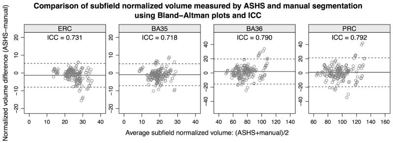
Bland-Altman plots and intraclass correlation coefficients (ICC) for the normalized volume of the ERC and the PRC subregions BA35 and BA36.

4. Evaluation of ASHS in the Context of Volumetric Group Difference Analysis in aMCI

4.1. Sub-Cohort Selection for Volumetry Analysis

Figure 7 illustrates the composition of the larger cohort used in the volumetric group difference analysis. Of the 92 subjects enrolled in the study, 29 were atlas subjects. Of the remaining 63 subjects, 57 passed image quality control for both T1-weighted and T2-weighted images; 5 had T2-weighted MRI with significant motion artifact; and one had a T2-weighted MRI with only partial coverage of the hippocampus. ASHS was trained using the 29 atlas subjects, and applied to segment the 57 non-atlas subjects who passed quality control. Visual inspection of ASHS segmentation results was performed, and in one subject, ASHS failed to label the hippocampal region (i.e., segmentation labels appeared elsewhere in the brain, as shown in Figure 7). The ASHS segmentations of the remaining 56 non-atlas subjects were available for analysis. Additionally, for the 29 subjects in the atlas set, the results of the cross-validation experiments were averaged to produce a single segmentation per subject. Specifically, if a subject had been segmented multiple times during cross-validation (since there were 90 experiments with 29 subjects, on average each subject had 3 segmentation attempts), the label posterior probability maps after the CL error correction step from the different segmentation attempts were averaged and used to produce a single consensus segmentation. Then the heuristic ERC/PRC post-processing step in Section 2.9 was applied to this consensus segmentation. After combining these averaged cross-validation segmentations of the 29 atlas subjects with the segmentations of the 56 non-atlas subjects, a total of 85 subjects with ASHS segmentations were available for analysis.

Figure 7.

Composition of the “full” cohort used in the volumetry and thickness analyses. The cohort combines the atlas set, for which segmentations produced using cross-validation are used, and most of the non-atlas subjects, which are segmented using ASHS trained on the atlas set. The bottom portion of the figure shows examples of the images excluded from the analysis. Please see text for details.

For extracting comparison measures, FreeSurfer was used to segment the T1-weighted MRI scans of these 85 subjects. Results were examined visually, and in two subjects (one atlas subject, one non-atlas subject), the FreeSurfer segmentations only partially covered the hippocampus. These two subjects were excluded from the subfield volumetry experiments. Thus, volumetry experiments were performed in the cohort of 83 subjects.

The demographic characteristics of this set of 83 subjects are presented in Table 5.

Table 5.

Summary of the composition of the full cohort and the atlas subset, including demographics, MRI coil used (8-channel or 32-channel), and cognitive testing. The p-values are two-tailed and computed using the t-test for numerical variables and using the Fisher exact test for sex and MRI coil.

	Full Cohort (n=83)					Atlas Subset (n=29)
	NC (n=43)		aMCI (n=40)		p	NC (n=15)		aMCI (n=14)		p
	Mean ± S.D.	Range	Mean ± S.D.	Range		Mean ± S.D.	Range	Mean ± S.D.	Range
Sex (male/female)	25 / 18		18 / 22		0.2752	7 / 8		6 / 8		1.0000
Age	71.0±9.6	54–88	71.8±7.0	56–85	0.6737	66.3±9.5	54–84	71.9±6.2	63–80	0.0696
Education (years)	16.5±2.9	12–20	16.6±2.7	12–20	0.9179	15.6±2.6	12–20	16.9±2.8	12–20	0.1994
MRI coil (8ch/32ch)	37 / 6		32 / 8		0.5624	15 / 0		14 / 0		1.0000
MMSE	29.4±0.9	27–30	27.3±1.8	22–30	0.0000	29.5±1.0	27–30	26.9±1.7	24–30	0.0001
CERAD word list total	23.8±3.6	16–30	16.4±4.1	8–24	0.0000	24.7±2.9	21–29	16.2±3.2	11–23	0.0000
Delayed Recall	8.4±1.6	4–10	3.6±2.1	0–8	0.0000	8.7±1.8	4–10	3.4±2.1	0–8	0.0000

Abbreviations: MMSE: Mini-Mental State Examination; CERAD: Consortium to Establish a Registry for Alzheimer’s Disease.

4.2. Subfield Volumetry Analysis Results

ASHS-derived volumes of hippocampal subfields and normalized volumes of the cortical subregions were compared statistically between the aMCI and NC groups. For each anatomical label, a general linear model (GLM) was fitted to the volumetric measurement of interest (i.e., volume or normalized volume), with group membership as the factor of interest. Age and ICV were included as covariates. The Student’s t-statistic and the p-value for the NC-aMCI contrast were computed from the fitted GLM for each anatomical label. Additionally, we computed the area under ROC curve (AUC) statistics for the NC-aMCI comparison after normalizing the dependent variable by age and ICV. This normalization was performed by fitting a GLM with the volumetric measurement as the dependent variable, age and ICV as independent variables, and taking the residuals.

The results of this statistical analysis are reported in the top panel of Table 6. On the left side, a significant group effect is found in all substructures except CA2, CA3 and SUB. The measures with the largest t-statistic and AUC values on the left side are the normalized volume of BA35 (t=4.80, AUC=0.784), the volume of the CA (t=4.45, AUC=0.785), followed by the PRC normalized volume (t=3.76, AUC=0.727) and the DG volume (t=3.58, AUC=0.730). The group difference for the left HIPP label (which combines CA, DG and SUB labels) is also very strong (t=4.20, AUC=0.763). On the right side, a similar picture emerges in the hippocampus, with largest group difference in CA (t=4.07, AUC=0.736) followed by DG difference (t=2.82, AUC=0.667). However, the strong effect in the BA35 is no longer present on the right side (t=1.58, AUC=0.622); in fact none of the right ERC/PRC measures reach significance.

Table 6.

Comparison of the size of hippocampal subfields and parahippocampal gyrus subregions between aMCI patients and controls, with age and ICV as covariates. The top panel of the figure lists summary statistics and group difference statistics for the different anatomical labels generated by ASHS, and the bottom panel lists corresponding statistics for the different FreeSurfer labels, which include substructures segmented by the Van Leemput et al. (2009) algorithm, as well as the whole hippocampus volume and ERC gray matter volume. For ASHS hippocampal subfield labels and all FreeSurfer labels, the statistics are computed on volume measurements. For ASHS parahippocampal gyrus subregions, the statistics are computed on volumes normalized by their extent in the slice direction (Equation 1).

For each label, the Table lists the mean and standard deviation of the measurement of interest (volume or normalized volume) in the aMCI (n=41) and NC (n=44) groups. These means and standard deviations are computed after the measures are corrected for age and ICV, as described in the text. For each label, the Table also gives the t-Statistic for the group difference between NC and aMCI, with age and ICV as covariates (82 degrees of freedom), as well as the corresponding p-value for a one-sided alternative hypothesis (aMCI < NC).

Lastly, for each label, the Table lists the area under the receiving operator characteristic curve (AUC). The AUC reflects the ability of the age and ICV-corrected measurements to discriminate between aMCI and NC conditions. The radius (half width) of the 95% confidence interval on the AUC, computed using the (DeLong et al., 1988) bootstrap-based method, is also given for each anatomical label.

ASHS
	Volume							Normalized Volume
	CA1	CA2	CA3	CA	DG	SUB	HIPP	ERC	BA35	BA36	PRC
Left Side
Mean (NC)	1241.80	14.86	62.30	1318.96	760.79	343.22	2422.97	25.04	19.82	80.75	100.47
Mean (MCI)	1089.93	13.81	56.68	1160.42	675.28	323.43	2159.12	22.84	16.16	71.01	87.13
SD (NC)	115.40	5.58	18.03	118.15	86.89	46.07	204.26	2.66	3.33	15.03	16.23
SD (MCI)	193.09	5.90	17.47	196.97	126.67	55.19	349.46	5.00	3.56	14.14	15.82
T-stat	4.35	0.83	1.43	4.45	3.58	1.76	4.20	2.51	4.80	3.01	3.76
P-value	4.0e-05	0.41	0.16	2.8e-05	0.00060	0.082	6.9e-05	0.014	7.3e-06	0.0035	0.00033
AUC	0.783	0.572	0.581	0.785	0.730	0.615	0.763	0.668	0.784	0.685	0.727
AUC 95% C.I. radius	0.102	0.126	0.125	0.101	0.111	0.123	0.108	0.121	0.102	0.116	0.109
Right Side
Mean (NC)	1258.97	21.29	72.43	1352.68	760.47	341.84	2455.00	24.26	19.42	69.38	88.74
Mean (MCI)	1117.07	18.27	64.17	1199.51	691.88	319.05	2210.44	22.95	17.94	69.66	87.51
SD (NC)	134.38	5.22	20.86	138.93	95.85	45.81	240.49	3.93	4.09	14.47	16.74
SD (MCI)	187.65	5.01	23.12	197.77	122.89	58.81	357.78	5.19	4.35	15.29	17.87
T-stat	3.95	2.66	1.70	4.07	2.82	1.96	3.65	1.29	1.58	−0.09	0.32
P-value	0.00017	0.0094	0.094	0.00011	0.0060	0.054	0.00047	0.20	0.12	0.93	0.75
AUC	0.726	0.645	0.605	0.736	0.667	0.615	0.709	0.585	0.622	0.478	0.504
AUC 95% C.I. radius	0.110	0.119	0.126	0.108	0.117	0.123	0.112	0.126	0.124	0.127	0.127

FreeSurfer
	PreSub	CA1	CA23	Fimb	Sub	DG	H. Fissure	H. Other	HIPP (FS)	ERC (FS)
Left Side
Mean (NC)	423.54	303.80	870.93	59.50	575.99	488.49	40.47	320.14	3727.28	1983.02
Mean (MCI)	382.88	300.66	800.24	47.14	518.65	445.27	45.21	306.60	3311.30	1747.60
SD (NC)	56.42	38.52	96.95	24.62	61.98	56.24	16.20	60.79	331.64	360.22
SD (MCI)	68.70	41.25	117.88	23.60	87.86	69.82	27.43	68.27	573.46	393.33
T-stat	2.93	0.36	2.97	2.31	3.43	3.09	−0.96	0.95	4.05	2.82
P-value	0.0044	0.72	0.0040	0.023	0.0010	0.0028	0.34	0.35	0.00012	0.0060
AUC	0.660	0.542	0.678	0.633	0.706	0.688	0.492	0.638	0.744	0.688
AUC 95% C.I. radius	0.119	0.128	0.117	0.121	0.116	0.117	0.130	0.125	0.110	0.119
Right Side
Mean (NC)	406.80	314.29	928.21	34.41	561.43	517.39	46.01	340.73	3710.02	1768.22
Mean (MCI)	390.77	304.59	844.73	28.73	527.25	473.94	47.65	325.60	3382.20	1698.44
SD (NC)	51.90	38.72	108.96	16.27	55.40	64.23	20.03	51.95	430.72	357.83
SD (MCI)	72.09	41.89	120.13	18.03	84.00	70.80	21.28	58.56	531.40	436.49
T-stat	1.16	1.09	3.29	1.49	2.18	2.91	−0.36	1.24	3.07	0.79
P-value	0.25	0.28	0.0015	0.14	0.032	0.0047	0.72	0.22	0.0029	0.43
AUC	0.566	0.576	0.706	0.598	0.642	0.683	0.485	0.595	0.693	0.526
AUC 95% C.I. radius	0.127	0.125	0.113	0.124	0.126	0.116	0.129	0.125	0.116	0.128

The bottom panel of Table 6 includes the results of group comparison using whole hippocampal volume, ERC grey matter volume, and hippocampal subfield volumes computed by FreeSurfer from the T1-weighted MRI in the same group of 83 subjects. The t-statistics obtained for the FreeSurfer whole hippocampal volume are slightly below those for the ASHS HIPP label (4.05 vs. 4.20 on the left, 3.07 vs. 3.65 on the right). The FreeSurfer ERC volume is significantly different between the groups only on the left, and the t-statistic for the left FreeSurfer ERC (2.82) is greater than for the ASHS ERC label (2.51) but smaller than for the ASHS BA35 label (4.80). Interestingly, for both the FreeSurfer ERC and the T2-based ERC/PRC, the group effect is only significant on the left side.

For the group differences computed using the Van Leemput et al. (2009) algorithm in FreeSurfer, t-statistics and AUCs for subfields in the left hippocampus are lower than those for FreeSurfer whole hippocampus volume (the left subiculum subfield has the highest statistics, with t = 3.43, AUC=0.706 vs. t = 4.05, AUC=0.744 for the whole hippocampus). On the right, the FreeSurfer CA23 subfield has higher t-statistic and AUC than FreeSurfer whole hippocampus volume (t = 3.29, AUC=0.706 vs. t = 3.07, AUC=0.693), and those statistics are just slightly less than for the ASHS CA volume (t = 4.07, AUC=0.736).

The covariates in the general linear model (age and ICV) were selected a priori, matching the statistical analysis performed in (Mueller et al., 2010). However, stepwise regression analysis using age, gender, education, MRI coil, and ICV as covariates and combined left and right hippocampal volume (computed using either FreeSurfer or ASHS) as dependent variables resulted in age, ICV and MRI coil being retained in the best fitting model, i.e., the model that yielded the lowest Bayesian Information Criterion (BIC). When the statistical analysis above was repeated with age, ICV, and MRI coil as covariates, the results were highly consistent with the ones reported in Table 6, with an overall slight increase in t-statistic and AUC for most structures. The largest overall t-statistics and AUCs remained in the left ASHS BA35 (t=4.95, AUC=0.785) and left ASHS CA (t=4.62, AUC=0.797) subfields, but on the right, the statistics for the FreeSurfer measures increased substantially more than for ASHS measures, bringing the two sets of measures much closer (right ASHS CA: t=4.29, AUC=0.743; right FreeSurfer CA23: t=3.89, AUC=0.749; right FreeSurfer DG: t=3.50, AUC=0.730).

Lastly, repeating the statistical analysis without covarying for age and ICV resulted in a slight reduction in the t-statistics and AUCs for most ASHS and FreeSurfer measurements, with the overall order of the statistics highly consistent with the results presented in Table 6.

5. Regional Subfield Thickness Analysis using ASHS

In addition to providing volume measures analyzed above, ASHS makes it possible to extract regional measures of subfield thickness and to analyze them in a common template space. This section describes the approach for thickness estimation (Section 5.1) and gives the results of regional comparison of subfield thickness between the aMCI and NC subjects (Section 5.2).

5.1. Methods for Regional Thickness Estimation in ASHS Output Segmentations

To complement global substructure volume measurements provided by ASHS with localized structural measurements, we perform additional image processing steps on the ASHS output. These steps include approximating ASHS segmentations with smooth boundaries, establishing correspondences between subjects, and extracting regional thickness maps.

5.1.1. Template-based Smooth Approximation for ASHS Segmentations

Because of the high voxel aspect ratio of the T2 images, the segmentations produced by ASHS (as well as manual segmentations) have a highly discontinuous surface with step edges (Figure 8A). Such discontinuities pose a challenge for shape analysis and extraction of thickness measures. Furthermore, statistical analysis of pointwise feature maps requires pointwise correspondences between all subjects’ segmentations, which are not produced by ASHS.

Figure 8.

Steps in the thickness computation pipeline. (A): a surface mesh of the combined segmentation of the CA, SUB, ERC and PRC structures in the right hemisphere in one subject; the step edges in the segmentation can be observed. (B): the surface mesh for the same set of structures in the unbiased population template constructed from 85 ASHS segmentations; the surface of the mesh is much smoother. (C): the smooth template surface warped to the space of the subject’s segmentation. (D): superimposition of the segmentation (A) and the warped template (C) showing that (C) provides a smooth approximation to (A). (E): Pruned Voronoi skeleton computed from the warped template surface. (F) Thickness (distance to the skeleton) mapped onto the boundary of the warped template.

To enable shape analysis, we apply a computational anatomy algorithm similar in spirit to the whole-hippocampal morphometry carried out in (Miller et al., 2005; Wang et al., 2007). For each hemisphere, an unbiased population template is constructed from the multi-label segmentations produced by ASHS. The approach is similar to the one used to build a template from the T1-weighted images in Section A.2, except that since the input images are multi-label segmentations rather than intensity images, a different image similarity metric is employed. Specifically, the mean square intensity difference metric is computed for each label separately, and the sum of these per-label metrics is minimized by the registration. The template resulting from this procedure has a very smooth surface, compared with the input segmentations (Figure 8B). By warping the template surface into the space of each input segmentation (using the diffeomorphic deformation fields generated during the construction of the unbiased template), we obtain a smooth and topologically consistent approximation of each input multi-label segmentation that is suitable for measuring regional thickness (Figure 8C,D).

5.1.2. Thickness Maps

Thickness maps are computed in the space of each subject from the smooth surfaces obtained above. Rather than computing a separate thickness map for each individual subfield or substructure, which would be problematic for smaller substructures and would cause a discontinuity in the thickness measurement along substructure boundaries, we combine substructures into two groups corresponding to the layered structure of the hippocampus. One group consists just of the DG subfield, while the other group, analogous to the (Zeineh et al., 2003; Ekstrom et al., 2009) hippocampus unfolding approach, combines all other subfields, i.e., the strip of gray matter encompassing the CA subfields, SUB, ERC and PRC (Figure 8B). Left and right hemispheres are analyzed separately. Given a smooth surface-based representation of a group of structures in a given subject’s space, thickness is computed for each surface point by extracting the Voronoi skeleton of the surface, pruning the skeleton to remove extraneous branches (Ogniewicz and Kübler, 1995)², and computing the distance from each point on the surface to the closest point on the pruned skeleton (Figure 8E,F). Lastly, thickness maps computed for each subject are mapped back into the space of the unbiased template for statistical analysis.

5.2. Results of Subfield Thickness Analysis in aMCI

Regional thickness analysis was applied to the output of ASHS segmentation in the cohort of 85 subjects (83 subjects analyzed in Section 4 plus the two subjects for whom FreeSurfer segmentation failed but the ASHS segmentation was acceptable). Surface representations of the DG label and the strip of tissue formed by combining the CA, SUB, ERC, BA35 and BA35 labels were extracted in template space and warped into the subject space, serving as a smooth interpolation of the corresponding structures in the ASHS segmentation output. The accuracy of the smooth interpolation was measured symmetric root mean square (RMS) surface distance (Gerig et al., 2001). For the surface combining the CA, SUB, ERC, BA35 and BA35 labels, the average symmetric RMS surface distance between the smooth interpolated surface (cyan surface in Figure 8D) and the surface of the ASHS segmentation (brown surface in Figure 8D) is 0.27±0.05 mm. For the surface of the DG, the average symmetric RMS distance is 0.19±0.04 mm.

Regional thickness maps computed for each subject using the smooth surface representations of the ASHS segmentations were brought back into the template space for statistical analysis. At each surface point, a general linear model (GLM) was fitted, with thickness at that point as the dependent variable, disease status as the factor of interest, and age and ICV as covariates. Figure 9 plots the map of the t-statistic for the NC-aMCI contrast derived from these point-wise GLMs. Uncorrected p-values were pooled across the four surfaces, and corrected for multiple comparisons using the False Discovery Rate (FDR) approach (Benjamini and Yekutieli, 2001).

Figure 9.

Surface-based statistical analysis of thickness differences between controls and aMCI patients, performed in the space of an unbiased population template derived from ASHS segmentation, and visualized from two different viewpoints. The top row shows the combined surface model composed of the CA, SUB, ERC, BA35 and BA36 subfields, with each vertex assigned the corresponding subfield label. The second row shows the DG, which is modeled as a separate surface. The third and fourth rows plot the t-statistic maps for the statistical comparison of thickness, with age and intracranial volume (ICV) as covariates, between NC and aMCI groups, carried out on these surface models. The dark outline on the t-statistic maps indicates the regions where the p-value is below 0.05 after false discovery rate (FDR) correction.

The uncorrected p-value corresponding to the FDR correction threshold of 0.05 is p = 0.0122, and corresponds to t = 2.29. Surface regions where the t-statistic exceeds this threshold are outlined by a bold black curve in Figure 9. The largest supra-threshold regions are (a) a region that includes most of the left BA35 and a large portion of the left ERC; and (b) a region along the infero-lateral aspect of the left CA, extending along most of the hippocampal head and body. The corresponding regions on the right are smaller: there are two large supra-threshold regions located in the right ERC, and two large regions along the inferio-lateral aspect of the right CA, one in the head, and another in the posterior part of the body and anterior part of the tail. Two small regions with high t-values are located on the superior portion of the right CA in the head, with smaller corresponding regions on the left. Also, the DG contains supra-threshold regions bilaterally in the posterior half of the structure. Overall, the thickness maps are consistent with the volumetric findings, but offer greater regional specificity.

6. Discussion

Segmentation of hippocampal subfields and parahippocampal gyrus subregions in in vivo MRI is a challenging problem and a subject of some debate. Recently, van Strien et al. (2009) argued that this problem is ill-posed because the features used by neuroanatomists to define subfield boundaries are primarily cytoarchitectonic and are not visible in MRI even at the highest possible resolution. For example, the anatomical boundary between CA1 and CA2 subfields is defined based on the differences in the size and density of pyramidal cells (Duvernoy, 2005). Such differences clearly cannot be observed using MRI. Van Strien et al. also caution against estimating subfield boundaries based on geometric rules because the location of the cytoarchitectonic boundaries relative to morphological features varies between individuals. Long-term efforts are currently under way to better relate 3D shape and appearance features extractable from postmortem MRI to the subfield boundaries extracted from histological data (Adler et al., 2013; Augustinack et al., 2013). If these efforts succeed in characterizing the relationship between MRI features and true histologically derived boundaries, in the future it may be possible to infer true subfield boundaries from MRI scans in a probabilistic way with certain guarantees of anatomical correctness.

However, the challenges identified by van Strien et al. (2009) have not prevented a number of groups from defining subfield segmentation protocols for in vivo MRI. These protocols are only approximations of the underlying anatomical truth, and must necessarily rely on a combination of available image intensity features and heuristic geometrical rules to derive a labeling scheme that is reliable and reproducible. One argument that can be made in favor of these protocols is that even though the substructures that they extract may be somewhat different in location and shape from the underlying true anatomical subfields, as long as such substructures yield additional information about the effects of disease on the hippocampus and MTL, or offer greater statistical power compared to alternative measures, they are useful as biomarkers. Moreover, these protocols are not completely removed from the underlying anatomy: even though some boundaries might be off with respect to the true anatomical boundaries, the subfields extracted from MRI overlap substantially with their true anatomical counterparts, particularly for larger subfields. Thus, as long as the results reported on the basis of MRI-derived subfield measurements are interpreted with the understanding that the measurements themselves are approximate, they are still useful for understanding MTL structure and function. Indeed, the uncertainty of anatomical boundaries is not unique to hippocampal subfields, and the critical points raised by van Strien et al. (2009) can also be directed at in vivo MRI segmentation of many other brain structures and cortical regions. Although uncertainty is a concern, it does not invalidate the use of in vivo MRI for studying brain structure and function.

Accepting the fact that there is a place in the field for in vivo MRI subfield measurements (as long as their approximate nature is properly recognized), it is natural to seek for such measurements to be obtained automatically. Although no algorithm will likely ever be able to mimic the deep intellectual process employed by a human expert when inferring and approximating subfield boundaries, manual segmentation also has significant limitations: it is far too costly for large datasets, is difficult to replicate between research groups, and is subject to various rater biases and temporal drifts. By contrast, automatic segmentation scales well to large datasets and is completely reproducible. Thus any additional inaccuracy arising from the use of automatic segmentation over the standard of manual segmentation must be weighted carefully against these benefits.

On the whole, our results show that ASHS has good consistency with manual segmentation, although there is room for improvement relative to the very high intra-rater reliability of the manual segmentation. Of course, echoing the concerns of van Strien et al. (2009), that finding in itself does not imply that ASHS is accurately segmenting the true underlying anatomical boundaries. Given this uncertainty, it is important to relate the ASHS results to knowledge about the pathology of the underlying disease. It is therefore encouraging that our finding of significant CA1 and left BA35 atrophy in aMCI is consistent with the expectations of AD-related change (Braak and Braak, 1995). Furthermore, our regional thickness analysis mitigates some of the criticisms raised by van Strien et al. (2009) because it is carried out on a region combining the CA, SUB, ERC and PRC substructures, and most of the boundary of this region with the DG is formed by the SRLM-HS, which is visible in the in vivo MRI. Thickness analysis makes it possible to identify regions of atrophy without having to assign them to a specific subfield label.

6.1. ASHS performance in cross-validation experiments

Given the highly complex nature of the subfield segmentation problem, we find the ability of ASHS to replicate manual segmentation of a number of structures (CA1, DG, PRC) with average DSC near or above 0.8 (Table 3) to be very encouraging. Nevertheless, there remains a considerable gap between these results and the intra-rater reliability of manual segmentation by rater JP, which for many subfields is in excess of 0.9. It is important to note that JP is the primary developer of our manual segmentation protocol, and has been involved in labeling hippocampal subfields in both in vivo and postmortem data for over seven years. On average, he spent over eight hours to segment each MRI scan. His intra-rater reliability is probably considerably higher than would be expected for a typical technician performing manual segmentation.

In fact, although the agreement between ASHS and manual segmentation falls short of the intra-rater reliability of rater JP, it is quite similar to the intra-rater reliability of manual segmentation reported elsewhere in the literature. For instance, Olsen et al. (2013) report mean DSC of 0.80 for CA1, 0.85 for combined DG, CA2 and CA3, and 0.78 for SUB for intra-rater reliability as well as 0.73 for CA1, 0.83 for DG/CA2/CA3, and 0.69 for SUB for inter-rater reliability. These subfields are traced through ¾ of the anterior-posterior extent of the hippocampus. The MRI protocol in Olsen et al. (2013) is similar to ours. Winterburn et al. (2013) report mean intra-rater reliability with DSC of 0.78 for CA1, 0.83 for CA4/DG, and 0.75 for SUB. Winterburn et al. (2013) performed manual segmentation in “dedicated” T2-weighted MRI scans with longer acquisition times and significantly lower slice thickness than the scans used in our paper. They segmented the hippocampus along its entire length, and their protocol includes a separate label for the SRLM-HS. Higher intra-rater overlaps (DSC of 0.85 for CA1, 0.84 for DG and SUB, 0.83 for CA2) are reported by Wisse et al. (2012), but in scans acquired at 7 Tesla with isotropic 0.7 × 0.7 × 0.7mm3 resolution. We emphasize that measures such as DSC cannot be directly compared between papers utilizing different MRI sequences and segmentation protocols, as the voxel size, number and complexity of the labels, and other factors can affect DSC significantly. Nonetheless, the fact that ASHS accuracy for larger subfields falls in the “ball park” of the intra-rater reliability reported by other authors is encouraging.

The agreement of ASHS and manual segmentation in the hippocampal body (Table 4: DSC of 0.878 for CA1, 0.594 for CA2, 0.431 for CA3, 0.892 for DG, 0.747 for SUB) is consistent with our earlier body-only automatic segmentation results (Yushkevich et al., 2010) and close to the inter-rater reliability reported in that paper (DSC of 0.883 for CA1, 0.522 for CA2, 0.668 for CA3, 0.885 for DG, 0.768 for SUB). The only exception is the CA3 subfield, for which reliability is much lower for ASHS; this is likely explained by the changes to the manual segmentation protocol that resulted in a smaller and thinner CA3 in the body, compared with the earlier protocol.

The agreement between ASHS and manual segmentation for the subfields in the head of the hippocampus (Table 4: DSC of 0.777 for CA1, 0.788 for DG) and the tail of the hippocampus (0.805 for CA1, 0.796 for DG) is considerably lower than in the hippocampal body (0.878 for CA1, 0.892 for DG). Certainly, the segmentation problem in the head and tail is more challenging than in the body because of much more complex shape of the subfields and the less consistent agreement between the slice direction and the hippocampal anatomy. In the tail, the intra-rater reliability of manual segmentation is also lower than in the body. However, in the head and body, the manual segmentation intra-rater reliability is approximately the same. Thus there is apparent room for improvement in the segmentation of head, which perhaps may be achieved using a larger number of atlases or through algorithmic enhancements.

For the ERC and the PRC subregions, the agreement of ASHS and manual segmentation reported in Table 3 (DSC = 0.786 for ERC, 0.702 for BA35, 0.777 for BA36, 0.797 for PRC) are not quite as high as for the larger hippocampal subfields (DSC = 0.803 for CA1, 0.823 for DG), and substantially lower than intra-rater reliability for rater JP. However, compared with other work, the reliability of ASHS falls within the range of published intra-rater reliability, and above published inter-rater reliability. For instance, in oblique coronal T2-weighted MRI at 3 Tesla, Olsen et al. (2013) report mean intra-rater DSC of 0.79 for the ERC and 0.78 for the PRC, with the inter-rater DSC of 0.71 for the ERC and 0.75 for the PRC. However, the anterior-posterior extent of the ERC/PRC segmentation is larger in Olsen et al. (2013). At 7 Tesla, Wisse et al. (2012), report intra-rater DSC of 0.83 for the ERC.

Overall, for the larger subfields, ASHS appears to perform quite well relative to published data on inter-rater reliability of manual segmentation, and is within the range of some published data on intra-rater reliability.

6.2. ASHS performance compared with other automatic segmentation methods

The literature on automatic segmentation of hippocampal subfields and parahippocampal gyrus subregions is relatively limited, and ASHS appears to perform quite competitively compared to earlier published methods.

Van Leemput et al. (2009) were the first to publish an automatic subfield segmentation technique, which was implemented and evaluated in ultra high-resolution T1-weighted images, obtained by averaging a set of five high-resolution T1-weighted MRI scans, acquired over the course of 35 minutes, that were motion-corrected and resampled to 0.38 × 0.38 × 0.38mm³ resolution. Van Leemput et al. (2009) label hippocampal subfields along the entire length of the hippocampus (except for about the most posterior 1/6th of the hippocampus, which is not partitioned into subfields). They evaluate their results against manual segmentation in 10 cognitively normal subjects. The largest mean DSC values reported by Van Leemput et al. (2009, Figure 3) are approximately 0.75 for the subiculum and 0.74 for CA2-3, with the other subfields having DSC below 0.7. ASHS accuracy relative to manual segmentation is slightly higher, with DSC exceeding 0.8 for subfields CA1 and DG, despite the fact that our evaluation is carried out in a cohort that includes patients with aMCI. Of course, any direct comparison of DSC between methods must take into account the differences in the segmentation protocol.

Although Van Leemput et al. (2009) technique was evaluated in ultra-high resolution MRI, its implementation in FreeSurfer has been primarily used to perform subfield volumetry in “routine” 1mm³ isotropic T1-weighted MRI scans (Hanseeuw et al., 2011; Engvig et al., 2012; Teicher et al., 2012; Lim et al., 2012). To our knowledge, the accuracy of the FreeSurfer subfield segmentation at that resolution relative to manual segmentation has not been evaluated, making a comparison with ASHS difficult. Given the difficulty in visualizing subfields at 1mm³ isotropic resolution (Figure 1), we would expect accuracy to be lower than what is reported by Van Leemput et al. (2009) for ultra-high resolution MRI. However, an inherent advantage of the FreeSurfer approach relative to ASHS is that it does not require collecting a dedicated T2-weighted MRI scan, which means that it can be applied to many more studies and is more robust to motion and other MRI artifacts. Furthermore, because it operates on scans with isotropic or nearly isotropic resolution, the segmentation approach in FreeSurfer does not have to account for heuristic segmentation rules based on slice boundaries in the way that ASHS does.

Flores et al. (2012) developed an automated technique for labeling hippocampal subfields in 7 Tesla MRI. The segmentation is performed in the hippocampal body, and the best mean DSC reported is 0.7 for DG. Other subfields have lower mean DSC, although the protocol employed does not trace all strata in the CA and SUB, which results in thinner segmentations and thus lower DSC.

Recently, Chakravarty et al. (2013) developed a technique MAGeT-Brain that emulates multi-atlas segmentation in problems where only a small number of expert-labeled atlases is available. Pipitone et al. (2014) evaluate this technique in the hippocampus and, in addition to reporting competitive accuracy for whole-hippocampus segmentation, demonstrate the feasibility of using MAGeT-Brain to label hippocampal subfields in “routine” 0.9x0.9x0.9 mm3 T1-weighted MRI scans. To measure accuracy, the authors perform cross-validation on manually segmented high-resolution scans from (Winterburn et al., 2012), resampled to the 0.9x0.9x0.9 mm3 resolution. Pipitone et al. (2014) report average DSC in the range of 0.55 to 0.65, good accuracy given the errors introduced by the resampling of the segmentations to lower resolution, as well as the fact that only three labeled atlases are used by the method. The performance of MAGeT-Brain hippocampal subfield segmentation directly in high-resolution T2-weighted “dedicated” MRI has not been reported, but if it could be shown to be comparable to that of multi-atlas segmentation as was shown for the case of whole hippocampus segmentation, that would make MAGeT-Brain an excellent alternative to ASHS, whose requirement of ~20 manually segmented atlas images for training may not always be practical or cost-effective.

For the ERC and PRC, there are not many papers reporting overlap between manual and automatic segmentation. Klein and Tourville (2012) report the mean DSC of 0.84 between FreeSurfer segmentation of the ERC (Desikan et al., 2006) and manual segmentation. FreeSurfer uses T1-weighted MRI and surface-based registration to infer the ERC boundaries, and the underlying manual segmentation leverages a surface-based protocol. On the other hand, the best-performing method in the 2012 Grand Challenge on Multi-Atlas Labeling (Landman and Warfield, 2012), which used volumetric registration of T1-weighted MRI, only attained DSC of 0.75 for the “entorhinal area” label. ASHS attained DSC of 0.786 for the ERC, although when overlap was computed just in the set of slices spanning the hippocampus head (Table 4), the DSC increased to 0.831. Overall, the extent and definition of ERC is quite different between these approaches, which makes it difficult to compare DSC values. However, the high accuracy reported by (Desikan et al., 2006) for the FreeSurfer ERC suggests that ASHS segmentation of ERC and PRC could be improved by incorporating features from surface-based analysis of cortical gray matter in the isotropic T1-weighted MRI. As noted below, tighter integration between T1-weighted and T2-weighted MRI is one of the main directions for future work.

This paper applied ASHS using a protocol that separates PRC into Brodmann areas 35 and 36. The ability to label BA35 was recently introduced into the FreeSurfer framework by Augustinack et al. (2013), who leveraged postmortem imaging to build a probability distribution on the location of BA35 on the cortical surface. The reliability of automatic segmentation of BA35 using surface-based mapping relative to manual segmentation is evaluated by Augustinack et al. (2013) in 7 postmortem tissue samples, and reported in terms of median Hausdorff distance: 4.0 mm for the left BA35 and 3.2 mm for the right BA35. The corresponding measures for ASHS, evaluated in the 29 images in the atlas set is 2.9 mm for the left BA35 and 2.9 mm for the right BA35. For BA36, the median Hausdorff distance is 3.5 mm on the left and 3.4 mm on the right. Of course, too much cannot be read into a comparison of segmentation performance of different methods employing different protocols in different kinds of data (postmortem vs. in vivo), but the numbers above indicate that ASHS does a reasonable job of mimicking the human’s segmentation of BA35 and BA36.

6.3. Effects of aMCI on the Hippocampal Region

The volumetric analysis of the effects of aMCI on the hippocampal subfields and the anterior subregions of the parahippocampal gyrus using ASHS is generally consistent with the earlier findings from in vivo T2-weighted MRI studies and with neuropathology findings. Utilizing manual segmentation of oblique coronal T2-weighted MRI in the body of the hippocampus, (Mueller et al., 2010) reported a trend for lower CA1 and SUB volume in MCI (not reaching significance) and a significant effect in the CA1-2 transition zone. La Joie et al. (2013) manually segmented CA1, SUB, and “other” label consisting of CA2, CA3 and DG along the whole length of the hippocampus, and reported strong effects in the CA1 and SUB subfields, weaker effects in the whole hippocampus, and no effects in the “other” label. In the current paper, the largest group effects in the hippocampus are observed in the left and right CA, with smaller effects in the DG, and smaller yet effects in SUB.

The finding of a strong group difference for the ASHS CA label is in keeping with these earlier papers and the pathological staging of AD by Braak and Braak (1995), who identify CA1 as the earliest site of neurofibrillary tangle (NFT) formation in the hippocampus. The overall strength of the group difference in the ASHS DG label is somewhat surprising. While we are unaware of any neuropathology studies that examine regional volume loss in aMCI, in an autopsy study of AD patients and age-matched controls, Simić et al. (1997) report that all hippocampal areas undergo volume loss, though this loss is most pronounced in the CA1 (43% loss), followed by SUB and CA2/3 (36% loss), and only then DG (16% loss). It is possible that ASHS is more sensitive to DG changes because DG segmentation is the most accurate, in terms of DSC and ICC, of all subfields. Furthermore, our segmentation protocol splits the SRLM-HS layer between CA1 and DG, rather than assigning this layer a separate anatomical label as done by some authors, e.g. Winterburn et al. (2013). In their analysis of 7 Tesla MRI, Kerchner et al. (2010) report that SRLM-HS volume was highly sensitive to AD status. Thus the partial inclusion of SRLM-HS into the DG label may explain its sensitivity to aMCI status in our study. In future work, it may prove useful to separately label SRLM-HS rather than assign its voxels to CA1 and DG.

The strong bilateral CA1 effect obtained using ASHS diverges from the findings of Hanseeuw et al. (2011) and Lim et al. (2012), who analyzed subfield volumes in “routine” T1-weighted MRI scans of aMCI patients and age-matched controls using the FreeSurfer implementation of the (Van Leemput et al., 2009) technique, and found differences in CA2-3, subiculum and, in the case of Lim et al., presubiculum, but not CA1. This discrepancy can be explained by the differences in the segmentation protocols between FreeSurfer (Van Leemput et al., 2009) and ASHS. The ASHS CA1 label is much larger, covering most of the FreeSurfer CA1 and subiculum labels, while the CA1 label in the FreeSurfer protocol is relatively small and corresponds to the most lateral portion of the CA1 in our protocol.

Our finding of a very strong effect in the left BA35 normalized volume (t=4.80, AUC=0.784) is very in keeping in pathology. Braak and Braak (1995) refer to BA35 as the “transentorhinal region” and describe it as the earliest site of NFT formation in the brain. Somewhat surprising is that this effect is only detected on the left side in our study. This asymmetry is also borne out in the FreeSurfer ERC gray matter volumes and the ASHS regional thickness analysis. Overall, all effects are stronger on the left than on the right, which might be explained by the fact that patients with left hippocampal atrophy whose verbal memory is impaired more greatly tend to seek out medical care more frequently than those with right hippocampal atrophy. Memory testing at the Penn Memory Center is weighted to the verbal domain, as it is at many specialty clinics. The finding of greater effects sizes in the left MTL than in the right is relatively common in the literature for MCI and AD (Shi et al., 2009).

In the comparison with the FreeSurfer subfield-specific, whole-hippocampus and ERC volume measurements, the highest AUC values and t-statistics for the aMCI and NC comparison were observed using ASHS subfield measurements (bilateral CA and left BA35). However, the differences in AUC are not large, and lie well within the width of the 95% confidence intervals on the AUCs (Table 6). A larger sample would be required to demonstrate that these differences in AUC are statistically significant. In the current sample, the DeLong et al. (1988) test yields p = 0.3 comparing the areas under the ROC curves for the ASHS measurement with the highest AUC (left CA volume, AUC=0.785) and the FreeSurfer measurement with the highest AUC (left hippocampus volume, AUC=0.744). A more comprehensive comparison will be possible using ADNI2 data (Mueller et al., 2013), which will have T1-weighted and oblique coronal T2-weighted MRI scans in over 200 subjects.

Regional analysis of hippocampal thickness reveals several “hot spots” for loss of thickness in aMCI relative to controls. These are generally consistent with the volumetric findings, with large clusters located on the left and right CA, a large cluster spanning ERC and the left BA35 in the fundus of the collateral sulcus, and several other smaller clusters. Although the idea of using surface maps to examine the effects of disease on hippocampal subfields is not new, previous surface-based techniques (Apostolova et al., 2006; Wang et al., 2006) analyzed the surface of the whole hippocampus, with the features projected on the surface not differentiated between the CA and DG, meaning that an effect detected on the hippocampal surface could be equally attributable to either of these subfields. By contrast, the surface maps in the current paper do not mix CA and DG, and allow the attribution of thickness clusters to specific subfields.

6.4. Limitations and Opportunities for Improvement

The key limitation of ASHS, which is also the key limitation of the underlying manual segmentation protocol, is the reliance on highly anisotropic, T2-weighted MRI scans tailored to imaging the MTL. Although these scans are becoming more and more common, and have recently been made part of the ADNI2 study (Mueller et al., 2013), they are much less ubiquitous than the whole-brain isotropic 1 mm³ T1-weighted scans, which means that ASHS cannot be leveraged for many past and ongoing imaging studies. Including such a T2-weighted scan adds 6–7 minutes to the MRI protocol, which may be challenging in the age when structural MRI has to compete for time with a host of functional and diffusion-weighted scans. Furthermore, the T2-weighted scans are much more affected by patient motion than the T1-weighted scans, and they require additional training for the MRI technicians. In our study, 6.5% of the scans had to be rejected due to patient motion. The rejection rate may be much higher in clinical settings. By contrast, none of the T1-weighted scans had to be excluded. The anisotropic nature of the T2-weighted scans poses challenges for defining the anterior-posterior extents of many structures, and in the current work, heuristic slice boundaries and normalized volume measurements for the ERC and the PRC substructures had to be imposed to deal with this limitation.

One possible way to address this limitation is by taking greater advantage of the isotropic T1-weighted MRI in the segmentation pipeline. The current approach uses T1-weighted MRI for initial alignment of the hippocampal region, but does not leverage it in later steps such as label fusion, corrective learning, and smooth interpolation. The isotropic nature of the T1 images can potentially complement the T2-weighted MRI, particularly when segmenting cortical structures. Lastly, T1-MRI can be useful for imposing sheet topology on the cortical structures, which in turn can allow for geometrical features to be leveraged during segmentation. Incorporating T1-MRI would require additional methodological development, such as multi-modality versions of the JLF and CL algorithms. Furthermore, if both modalities are used during atlas-to-target registration, one must either determine the proper weighting for these modalities in the registration objective function, or pass as input to label fusion the results of multiple atlas-to-target registrations performed with different weighting. Furthermore, for T1-MRI to be useful in avoiding partial volume effects in cortical structures due to thick slices in T2-MRI, the manual segmentations, which themselves currently suffer from the partial volume problem, would have to be done in a combination of the two modalities, which is a non-trivial problem.

Our current segmentation protocol does not include the parahippocampal cortex (PHC), and the extent of the ERC and PRC is limited to a slab of slices around the hippocampal head. In future work, we intend to incorporate PHC and extend the ERC/PRC segmentation further in the anterior direction, similar to the work of (Ekstrom et al., 2009; Olsen et al., 2013) and others.

A limitation of the segmentation cross-validation experiments in Section Error! Reference source not found. is that they only consider a single MRI protocol and a single manual segmentation protocol. As a result, the experiments do not evaluate the ability of ASHS to generalize to new MRI protocols and new segmentation protocols, even though ASHS supports such generalization by providing a training module. In particular, even though we use 32-channel data in the MCI-NC comparison in Section Error! Reference source not found., the accuracy of ASHS relative to manual segmentation in this data is not known, as we did not have manual segmentations to which to compare. Evaluation of ASHS on new MRI protocols and new segmentation protocols will be part of future work. It is possible that some segmentation protocols would require ASHS to be extended. For instance, protocols that label the SRLM-HS as a very thin structure, such as (Winterburn et al. , 2013), might benefit from a modification that imposes topology and/or shape constraints on ASHS segmentations.

A limitation of the thickness analysis is that it constructs a single template from all segmentations, and thus does not account for variability in gyral and sulcal patterns, which is particularly significant in the PRC, for which Ding and Van Hoesen (2010) describe three distinct anatomical variants based on the branching of the collateral sulcus. In future work, the possibility of stratifying subjects into groups based on the variants of PRC will be investigated.

ASHS is computationally expensive and requires a substantial number of parameters to be set, mostly empirically. Although it is possible to run ASHS segmentation on a single CPU, training ASHS in a practical length of time requires a multi-node computing cluster. It is possible to optimize some of the ASHS parameters by using an additional layer of cross-validation on the atlas set, but this would increase the computation time and risks overfitting the parameter settings to a particular dataset, imaging protocol, or segmentation protocol. In preparing this paper, little parameter tweaking took place either for speed or accuracy.³

7. Conclusion

ASHS is a fully automatic algorithm for labeling hippocampal subfields and adjacent cortical subregions in oblique coronal T2-weighted MRI scans. Although such scans are not as commonly acquired as the isotropic T1-weighted MRI, they can be easily incorporated into research and clinical imaging studies at the cost of under seven minutes of additional scanning time. ASHS builds on earlier work that performed well for labeling subfields in the hippocampal body (Yushkevich et al., 2010), and introduces several improvements, most importantly, the ability to label subfields along the entire anterior-posterior extent of the hippocampus. Although the performance of ASHS vis-a-vis manual segmentation does not match the intra-rater reliability of the rater on whose segmentations the method was trained, it is competitive with published data on inter-rater reliability of manual segmentation and published evaluations of other automatic subfield segmentation techniques. When applied to data from a study of aMCI, the algorithm produces sensible results, with bilateral CA1 and left BA35 being the anatomical labels most significantly different between patients and controls, although, somewhat surprisingly, DG is also significantly different and right ERC/PRC not reaching significance. In addition to producing volume information, the algorithm provides regional thickness measurements, which provide a more detailed picture of the effects of aMCI on the hippocampal region. The software implementation of ASHS is provided in the public domain n and makes it possible to retrain the algorithm using other imaging data and segmentation protocols.

Table 7.

Accuracy of ASHS segmentation relative to manual segmentation, measured in terms of symmetric root mean squared surface distance (Gerig et al., 2001), as opposed to Dice similarity coefficient, which measures volumetric overlap. Smaller or thinner structures, such as CA2 and SUB, tend do have lower Dice coefficient than larger or thicker structures with similar distance errors.

Metric	CA1	CA2	CA3	CA	DG	SUB	ERC	BA35	BA36	PRC	HIPP
Symmetric RMS surface distance (mm) Smaller = Better	0.529	0.670	0.856	0.505	0.560	0.511	0.675	0.799	0.859	0.790	0.480
Relative volume overlap (DSC) Larger = Better	0.803	0.552	0.525	0.797	0.823	0.750	0.786	0.702	0.777	0.797	0.893

Appendix

A. ASHS Training Pipeline Details

This appendix provides additional details about the implementation of the ASHS training pipeline described in Section 2.7. Each section below expands on the corresponding step in Section 2.7.

A.1. Rigid Alignment of T1- and T2-Weighted MRI

The purpose of this step is to bring the T1 and T2-weighted scans of each subject into close alignment, correcting for subject motion that may have taken place between the scans. To maximize robustness to registration failure, alignment is performed using both FLIRT (Smith et al., 2004) and ANTS (Avants et al., 2008a) rigid registration algorithms, using the normalized mutual information (NMI) metric as the similarity measure. The method that yields the largest NMI value between the two modalities is used subsequently. ⁴

A.2. Deformable Registration of T1-weighted MRI to an Unbiased Template

T1-weighted MRI from all atlas subjects are used to construct an unbiased population template using the ANTS affine and high-dimensional deformable registration algorithms (Avants et al., 2008a) and the diffeomorphic image averaging approach (Joshi et al., 2004; Avants and Gee, 2004). This approach alternates between averaging the intensity of all images and registering all images to the intensity average. In our implementation, this is repeated for four iterations (more details about the parameters of the algorithm are provided in Table 8). Beyond four iterations, gains in groupwise registration are negligible with respect to the overall goal of the template construction, which is to allow localization of the left and right hippocampal regions.

Table 8.

Key parameters used by ASHS. Parameters of ANTS and other algorithms that do not appear in the table are set to their defaults in the corresponding software implementation.

Parameter	Value
Whole-brain T1-w MRI registration and template construction
ANTS optimization iterations (specified as the number of iterations at 4x subsampling, 2x subsampling, and full resolution, respectively)	60×20×0
Template-building iterations (i.e., number of times averaging and registration to average are alternated)	4
Regional T2-weighted MRI registration
ANTS optimization iterations	60×60×20
Joint Label Fusion
Patch size for estimating expected joint segmentation error, i.e. the size of N(x) in (Wang et al., 2012, Eqn. 18)	7×7×3 voxels
Window size for the local search algorithm, i.e., the size of N'(x) in (Wang et al., 2012, Eqn. 19)	7×7×3 voxels
Corrective Learning
Number of iterations of AdaBoost training	500
Maximum number of voxels sampled for training each classifier	100000
Size of the patch used to sample intensity features for the classifier	13×13×1 voxels

A.3. Construction of Left and Right Hippocampal ROIs in Template Space

For each hemisphere, a mask is computed in the template space. To compute the mask, for each subject, all the left or right labels in the manual segmentation are combined into a single label, and the combined segmentation is deformed into the space of the template. The segmentations from all subjects are averaged and a threshold is applied to extract a mask. To extract an ROI for each hemisphere, the mask is dilated using a spherical structuring element with 1cm radius, and a rectangular box containing the dilated mask is extracted. The template ROIs are then supersampled to 0.4 × 0.4 × 0.4 mm³ resolution. The T2-weighted scan from each subject is resampled into the space of each ROI by composing the T2-to-T1 rigid transformation from Step 1 and the T1-to-template deformable transformation from Step 2.

A.4. Step 4: Training of CL Classifiers via Leave-One-Out Segmentation

This step involves generating a leave-one-out automatic segmentation of each subject’s left and right hippocampus, followed by the training of CL classifiers. Without loss of generality, we describe the procedure for the left hemisphere.

For every pair of subjects in the atlas package, ANTS deformable registration is performed between their respective T2-weighed MRI scans resampled into the space of the left template ROI. Such ROI-limited deformable registration between pairs of atlases has a greater chance of successfully aligning substructures in the hippocampal region than direct registration between raw T2-weighted images, as the registration problem is much better initialized, with the hippocampal regions brought into alignment by the groupwise whole-brain T1 registration in Step 2. Furthermore, restricting registration to an ROI around the hippocampus greatly reduces computation time. Registration is performed using the Symmetric Normalization (SyN) algorithm in ANTS (Avants et al., 2008b), with normalized cross-correlation used as the similarity metric.

Next, a leave-one-out segmentation of each atlas subject k is computed using the JLF algorithm. For each subject m (m ≠ k), the T2-weighted MRI of subject m and its corresponding manual segmentation are resampled into the space of the T2-weighted MRI of subject k by composing five transformations: the T2-to-T1 rigid transformation for subject k; the T1-to-template transformation for subject k; the resampled T2 to resampled T2 transformation between subjects k and m; the inverse T1-to-template transformation for subject m; and the inverse T2-to-T1 transformation for subject m. The resulting N-1 warped T2-weighted scans and N-1 warped segmentations are input into the JLF algorithm to produce a multi-atlas segmentation of the left hemisphere in the T2-weighted scan of subject k.

As the result, for each subject in the atlas, we obtain a leave-one-out multi-atlas segmentation of the structures of interest in the left hemisphere. These segmentations, along with the corresponding manual segmentations of the atlas subjects and the T2-weighted MRI scans themselves are used as input to train the corrective learning (CL) classifiers, as described in (Wang et al., 2010).

B. ASHS Segmentation Pipeline Details

This appendix provides additional details about the implementation of the ASHS segmentation pipeline described in Section 2.8. Each section below expands on the corresponding step in Section 2.8.

B.1. Within-Subject Multi-Modality Alignment

Alignment of the new subject’s T2-weighted MRI to his or her T1-weighted MRI uses the same approach as in the ASHS training pipeline (Section A.1).

B.2. Registration to the Whole-Brain T1-MRI Template

The new subject’s T1-weighted MRI image is registered to the whole-brain T1-weighted MRI template contained in the atlas package (produced in Section A.2) using the SyN algorithm (Avants et al., 2008b) with the same affine and deformable registration parameters as when constructing the template. The resulting deformation is then used to resample the target subject’s T1 and T2 images into the space of the left and right hippocampal ROIs in the template.

B.3. Localized Deformable Registration of Atlas T2-Weighted MRIs to the New Subject

Deformable registration is performed in the space of the left and right hippocampal ROIs in the template, between the resampled T2-weighted MRI of the new subject and each of the resampled T2-weighted images from the atlas package. Same registration parameters as in Section A.4 are used.

B.4. Multi-Atlas JLF Segmentation and CL Error Correction

Multi-label segmentations from each of the atlas images are warped into the space of the target T2-weighted image by composing the warps and linear transformations between it and each of the atlas T2-weighted images (in all, five transformations are composed: target T2 to target T1; target to whole-brain template; target (resampled to template space) to atlas (resampled to template space); whole-brain template to atlas; atlas T1 to atlas T2). The JLF algorithm is applied to obtain posterior probability maps for each label in the target T2-weighted image. These posteriors, and the target T2-weighted image itself, are input to the CL classifiers, which yield corrected posterior probability maps for each label. A binary segmentation of the T2-weighted image is obtained by assigning the label with highest posterior value to each voxel.

B.5. Bootstrapping

The bootstrapping step is added to improve segmentation quality by making sure that a large fraction of the atlas-to-target registrations are of adequate quality. Problems with local minima and poor initialization cause many of the pairwise registrations between the atlases and the target image to misalign structures in the hippocampal region. While JLF can cope with the presence of poor registrations, overall performance is better when the underlying registrations are themselves improved. During the bootstrapping step, the segmentations obtained at the previous step are used to guide the registration between the target image and each of the atlases. Specifically, in each hemisphere, affine registration between the target image and the atlas is computed using robust point matching affine registration (Papademetris et al., 2003) between points sampled from the surface of the automatic segmentation of the target image and points sampled from the surface of the manual segmentation of the atlas. The similarity measure optimized by this registration is computed separately for each label, i.e., CA1 points are matched to CA1 points, etc. Using the affine registration between segmentation surfaces as the initialization, regional deformable image registration between the atlas and target T2-weighted images is performed, employing the same method and parameters as in Section B.3. Lastly, multi-atlas JLF segmentation and CL error correction (Section B.4) are repeated using the transformations computed in the bootstrap step.

C. Segmentation Similarity Metrics

Dice Similarity Coefficient (DSC): for a pair of segmentations S_a and S_b and a given label l, the DSC is given as

$$\text{DSC}(S_a,S_b;l)=2\frac{\mid \{x\in \mathrm{\Omega }:S_a(x)=S_b(x)=l\}\mid }{\mid \{x\in \mathrm{\Omega }:S_a(x)=l\}\mid +\mid \{x\in \mathrm{\Omega }:S_b(x)=l\}\mid }$$

(Dice, 1945),where Ω is the set of all voxel indices in the image.

Generalized Dice Similarity Coefficient (GDSC): for a pair of segmentations S_a and S_b and a set of foreground labels L_fg, GDSC (Crum et al., 2006) is computed as

$$\text{GDSC}(S_a,S_b)=2\frac{\mid \{x\in \mathrm{\Omega }:S_a(x)=S_b(x)\in L_{\text{fg}}\mid }{\mid \{x\in \mathrm{\Omega }:S_a(x)\in L_{\text{fg}}\}\mid +\mid \{x\in \mathrm{\Omega }:S_b(x)\in L_{\text{fg}}\}\mid }.$$

References

- Adler DH, Pluta J, Kadivar S, Craige C, Gee JC, Avants BB, Yushkevich PA. Histology-derived volumetric annotation of the human hippocampal subfields in postmortem MRI. Neuroimage. 2013 doi: 10.1016/j.neuroimage.2013.08.067. [DOI] [PMC free article] [PubMed] [Google Scholar]
- Aljabar P, Heckemann RA, Hammers A, Hajnal JV, Rueckert D. Multi-atlas based segmentation of brain images: atlas selection and its effect on accuracy. Neuroimage. 2009;46:726–738. doi: 10.1016/j.neuroimage.2009.02.018. [DOI] [PubMed] [Google Scholar]
- Apostolova LG, Dinov ID, Dutton RA, Hayashi KM, Toga AW, Cummings JL, Thompson PM. 3D comparison of hippocampal atrophy in amnestic mild cognitive impairment and Alzheimer’s disease. Brain. 2006;129:2867–2873. doi: 10.1093/brain/awl274. [DOI] [PubMed] [Google Scholar]
- Artaechevarria X, Munoz-Barrutia A, Ortiz-de Solorzano C. Combination strategies in multi-atlas image segmentation: application to brain MR data. IEEE Trans Med Imaging. 2009;28:1266–1277. doi: 10.1109/TMI.2009.2014372. [DOI] [PubMed] [Google Scholar]
- Augustinack JC, Huber KE, Stevens AA, Roy M, Frosch MP, van der Kouwe AJW, Wald LL, Van Leemput K, McKee AC, Fischl B Alzheimer’s Disease Neuroimaging Initiative. Predicting the location of human perirhinal cortex, brodmann’s area 35, from MRI. Neuroimage. 2013;64:32–42. doi: 10.1016/j.neuroimage.2012.08.071. [DOI] [PMC free article] [PubMed] [Google Scholar]
- Avants B, Epstein C, Grossman M, Gee J. Symmetric diffeomorphic image registration with cross-correlation: Evaluating automated labeling of elderly and neurodegenerative brain. Medical Image Analysis. 2008a;12:26–41. doi: 10.1016/j.media.2007.06.004. [DOI] [PMC free article] [PubMed] [Google Scholar]
- Avants B, Gee JC. Geodesic estimation for large deformation anatomical shape averaging and interpolation. Neuroimage. 2004;23(Suppl 1):S139–S150. doi: 10.1016/j.neuroimage.2004.07.010. [DOI] [PubMed] [Google Scholar]
- Avants BB, Epstein CL, Grossman M, Gee JC. Symmetric diffeomorphic image registration with cross-correlation: evaluating automated labeling of elderly and neurodegenerative brain. Med Image Anal. 2008b;12:26–41. doi: 10.1016/j.media.2007.06.004. [DOI] [PMC free article] [PubMed] [Google Scholar]
- Bakker A, Kirwan CB, Miller M, Stark CEL. Pattern separation in the human hippocampal CA3 and dentate gyrus. Science. 2008;319:1640–2. doi: 10.1126/science.1152882. [DOI] [PMC free article] [PubMed] [Google Scholar]
- Benjamini Y, Yekutieli D. The control of the false discovery rate in multiple testing under dependency. The Annals of Statistics. 2001;29:1165–1188. [Google Scholar]
- Bland J, Altman D. Agreement between methods of measurement with multiple observations per individual. J Biopharm Stat. 2007;17:571–582. doi: 10.1080/10543400701329422. [DOI] [PubMed] [Google Scholar]
- Bobinski M, Wegiel J, Tarnawski M, Bobinski M, Reisberg B, de Leon MJ, Miller DC, Wisniewski HM. Relationships between regional neuronal loss and neurofibrillary changes in the hippocampal formation and duration and severity of Alzheimer disease. J Neuropathol Exp Neurol. 1997;56:414–420. doi: 10.1097/00005072-199704000-00010. [DOI] [PubMed] [Google Scholar]
- Bonnici HM, Chadwick MJ, Kumaran D, Hassabis D, Weiskopf N, Maguire EA. Multi-voxel pattern analysis in human hippocampal subfields. Front Hum Neurosci. 2012;6:290. doi: 10.3389/fnhum.2012.00290. [DOI] [PMC free article] [PubMed] [Google Scholar]
- Braak H, Braak E. Staging of Alzheimer’s disease-related neurofibrillary changes. Neurobiol Aging. 1995;16:271–8. doi: 10.1016/0197-4580(95)00021-6. discussion 278–84. [DOI] [PubMed] [Google Scholar]
- Breyer T, Wanke I, Maderwald S, Woermann F, Kraff O, Theysohn J, Ebner A, Forsting M, Ladd M, Schlamann M. Imaging of patients with hippocampal sclerosis at 7 Tesla: initial results. Academic radiology. 2010;17:421–426. doi: 10.1016/j.acra.2009.10.013. [DOI] [PubMed] [Google Scholar]
- Chakravarty MM, Steadman P, van Eede MC, Calcott RD, Gu V, Shaw P, Raznahan A, Collins DL, Lerch JP. Performing label-fusion-based segmentation using multiple automatically generated templates. Hum Brain Mapp. 2013;34(10):2635–54. doi: 10.1002/hbm.22092. [DOI] [PMC free article] [PubMed] [Google Scholar]
- Cho Z, Han J, Hwang S, Kim D, Kim K, Kim N, Kim S, Chi J, Park C, Kim Y. Quantitative analysis of the hippocampus using images obtained from 7.0 T MRI. Neuroimage. 2010;49:2134–2140. doi: 10.1016/j.neuroimage.2009.11.002. [DOI] [PubMed] [Google Scholar]
- Crum WR, Camara O, Hill DLG. Generalized overlap measures for evaluation and validation in medical image analysis. IEEE Trans Med Imaging. 2006;25:1451–61. doi: 10.1109/TMI.2006.880587. [DOI] [PubMed] [Google Scholar]
- DeLong E, DeLong D, Clarke-Pearson D. Comparing the areas under two or more correlated receiver operating characteristic curves: a nonparametric approach. Biometrics. 1988:837–845. [PubMed] [Google Scholar]
- Desikan RS, Ségonne F, Fischl B, Quinn BT, Dickerson BC, Blacker D, Buckner RL, Dale AM, Maguire RP, Hyman BT, Albert MS, Killiany RJ. An automated labeling system for subdividing the human cerebral cortex on mri scans into gyral based regions of interest. Neuroimage. 2006;31:968–80. doi: 10.1016/j.neuroimage.2006.01.021. [DOI] [PubMed] [Google Scholar]
- Ding SL, Van Hoesen GW. Borders, extent, and topography of human perirhinal cortex as revealed using multiple modern neuroanatomical and pathological markers. Hum Brain Mapp. 2010;31:1359–79. doi: 10.1002/hbm.20940. [DOI] [PMC free article] [PubMed] [Google Scholar]
- Duvernoy H. The Human Hippocampus: Functional Anatomy, Vascularization and Serial Sections with MRI. Berlin, Germany: Springer; 2005. [Google Scholar]
- Eichenbaum H, Yonelinas AR, Ranganath C. The Medial Temporal Lobe and Recognition Memory. Annu Rev Neurosci. 2007;30:123–52. doi: 10.1146/annurev.neuro.30.051606.094328. [DOI] [PMC free article] [PubMed] [Google Scholar]
- Ekstrom AD, Bazih AJ, Suthana NA, Al-Hakim R, Ogura K, Zeineh M, Burggren AC, Bookheimer SY. Advances in high-resolution imaging and computational unfolding of the human hippocampus. Neuroimage. 2009;47:42–9. doi: 10.1016/j.neuroimage.2009.03.017. [DOI] [PMC free article] [PubMed] [Google Scholar]
- Engvig A, Fjell AM, Westlye LT, Skaane NV, Sundseth O, Walhovd KB. Hippocampal subfield volumes correlate with memory training benefit in subjective memory impairment. Neuroimage. 2012;61:188–94. doi: 10.1016/j.neuroimage.2012.02.072. [DOI] [PubMed] [Google Scholar]
- Fischl B. Freesurfer. Neuroimage. 2012 doi: 10.1016/j.neuroimage.2012.01.021. [DOI] [PMC free article] [PubMed] [Google Scholar]
- Flores GS, de Haan G, Jasinschi R, Soldea O. Master’s thesis. Technische Universiteit Eindhoven; 2012. Automatic Segmentation of Hippocampal Substructures. [Google Scholar]
- Freund Y, Schapire R. A decision-theoretic generalization of on-line learning and an application to boosting. Computational Learning Theory: Second European Conference, EuroCOLT’95; Barcelona, Spain. March 13–15, 1995; Springer; 1995. p. 23. Proceedings. [Google Scholar]
- Gerig G, Jomier M, Chakos M. Medical Image Computing and Computer-Assisted Intervention–MICCAI. Vol. 2001. Springer; Berlin Heidelberg: 2001. Valmet: A new validation tool for assessing and improving 3D object segmentation; pp. 516–523. [Google Scholar]
- Hanseeuw BJ, Van Leemput K, Kavec M, Grandin C, Seron X, Ivanoiu A. Mild cognitive impairment: differential atrophy in the hippocampal subfields. AJNR Am J Neuroradiol. 2011;32:1658–61. doi: 10.3174/ajnr.A2589. [DOI] [PMC free article] [PubMed] [Google Scholar]
- Heckemann RA, Keihaninejad S, Aljabar P, Rueckert D, Hajnal JV, Hammers A Alzheimer’s Disease Neuroimaging Initiative. Improving intersubject image registration using tissue-class information benefits robustness and accuracy of multi-atlas based anatomical segmentation. Neuroimage. 2010;51:221–7. doi: 10.1016/j.neuroimage.2010.01.072. [DOI] [PubMed] [Google Scholar]
- Henry TR, Chupin M, Lehéricy S, Strupp JP, Sikora MA, Sha ZY, Ugurbil K, Van de Moortele PF. Hippocampal sclerosis in temporal lobe epilepsy: findings at 7 t. Radiology. 2011;261:199–209. doi: 10.1148/radiol.11101651. [DOI] [PMC free article] [PubMed] [Google Scholar]
- Iglesias JE, Sabuncu MR, Van Leemput K Alzheimer’s Disease Neuroimaging Initiative. Improved inference in bayesian segmentation using monte carlo sampling: application to hippocampal subfield volumetry. Med Image Anal. 2013;17:766–78. doi: 10.1016/j.media.2013.04.005. [DOI] [PMC free article] [PubMed] [Google Scholar]
- Joshi S, Davis B, Jomier M, Gerig G. Unbiased diffeomorphic atlas construction for computational anatomy. Neuroimage. 2004;23(Suppl 1):S151–S160. doi: 10.1016/j.neuroimage.2004.07.068. [DOI] [PubMed] [Google Scholar]
- Kerchner G, Hess C, Hammond-Rosenbluth K, Xu D, Rabinovici G, Kelley D, Vigneron D, Nelson S, Miller B. Hippocampal CA1 apical neuropil atrophy in mild alzheimer disease visualized with 7-T MRI. Neurology. 2010;75:1381–1387. doi: 10.1212/WNL.0b013e3181f736a1. [DOI] [PMC free article] [PubMed] [Google Scholar]
- Kirov II, Hardy CJ, Matsuda K, Messinger J, Cankurtaran CZ, Warren M, Wiggins GC, Perry NN, Babb JS, Goetz RR, George A, Malaspina D, Gonen O. In vivo 7 tesla imaging of the dentate granule cell layer in schizophrenia. Schizophrenia Research. 2013 doi: 10.1016/j.schres.2013.04.020. [DOI] [PMC free article] [PubMed] [Google Scholar]
- Klein A, Tourville J. 101 labeled brain images and a consistent human cortical labeling protocol. Front Neurosci. 2012;6:171. doi: 10.3389/fnins.2012.00171. [DOI] [PMC free article] [PubMed] [Google Scholar]
- La Joie R, Fouquet M, Mézenge F, Landeau B, Villain N, Mevel K, Pélerin A, Eustache F, Desgranges B, Chételat G. Differential effect of age on hippocampal subfields assessed using a new high-resolution 3T MR sequence. Neuroimage. 2010;53:506–514. doi: 10.1016/j.neuroimage.2010.06.024. [DOI] [PubMed] [Google Scholar]
- La Joie R, Perrotin A, de La Sayette V, Egret S, Doeuvre L, Belliard S, Eustache F, Desgranges B, Chételat G. Hippocampal subfield volumetry in mild cognitive impairment, alzheimer’s disease and semantic dementia. NeuroImage: Clinical. 2013;3:155–162. doi: 10.1016/j.nicl.2013.08.007. [DOI] [PMC free article] [PubMed] [Google Scholar]
- Landman BA, Warfield SK, editors. MICCAI 2012 Workshop on Multi-Atlas Labeling. CreateSpace. 2012 https://masi.vuse.vanderbilt.edu/workshop2012/images/c/c8/MICCAI_2012_Workshop_v2.pdf.
- Libby LA, Ekstrom AD, Ragland JD, Ranganath C. Differential connectivity of perirhinal and parahippocampal cortices within human hippocampal subregions revealed by high-resolution functional imaging. J Neurosci. 2012;32:6550–60. doi: 10.1523/JNEUROSCI.3711-11.2012. [DOI] [PMC free article] [PubMed] [Google Scholar]
- Lim HK, Hong SC, Jung WS, Ahn KJ, Won WY, Hahn C, Kim IS, Lee CU. Automated hippocampal subfield segmentation in amnestic mild cognitive impairments. Dement Geriatr Cogn Disord. 2012;33:327–33. doi: 10.1159/000339588. [DOI] [PubMed] [Google Scholar]
- Malykhin NV, Lebel RM, Coupland NJ, Wilman AH, Carter R. In vivo quantification of hippocampal subfields using 4.7 T fast spin echo imaging. Neuroimage. 2010;49:1224–1230. doi: 10.1016/j.neuroimage.2009.09.042. [DOI] [PubMed] [Google Scholar]
- Miller MI, Beg MF, Ceritoglu C, Stark C. Increasing the power of functional maps of the medial temporal lobe by using large deformation diffeomorphic metric mapping. Proc Natl Acad Sci U S A. 2005;102:9685–9690. doi: 10.1073/pnas.0503892102. [DOI] [PMC free article] [PubMed] [Google Scholar]
- Mueller S, Stables L, Du A, Schuff N, Truran D, Cashdollar N, Weiner M. Measurements of hippocampal subfields and age related changes with high resolution MRI at 4T. Neurobiology of Aging. 2007a;28:719–726. doi: 10.1016/j.neurobiolaging.2006.03.007. [DOI] [PMC free article] [PubMed] [Google Scholar]
- Mueller SG, Schuff N, Raptentsetsang S, Stables L, Weiner MW. Distinct atrophy pattern in hippocampal subfields in Alzheimer’s disease (AD) and mild cognitive impairment (MCI) Alzheimer’s and Dementia. 2007b;3:S113. [Google Scholar]
- Mueller SG, Schuff N, Yaffe K, Madison C, Miller B, Weiner MW. Hippocampal atrophy patterns in mild cognitive impairment and Alzheimer’s disease. Hum Brain Mapp. 2010;31:1339–47. doi: 10.1002/hbm.20934. [DOI] [PMC free article] [PubMed] [Google Scholar]
- Mueller SG, Weiner MW. Selective effect of age, Apo e4, and Alzheimer’s disease on hippocampal subfields. Hippocampus. 2009;19:558–564. doi: 10.1002/hipo.20614. [DOI] [PMC free article] [PubMed] [Google Scholar]
- Mueller SG, Yushkevich PA, Wang L, Van Leemput K, Mezher A, Das SR, Iglesias JE, Weiner MW. Collaboration for a systematic comparison of different techniques to measure subfield volumes: Announcement and first results. Alzheimer’s Association International Conference (AAIC).2013. [Google Scholar]
- Norman KA. How hippocampus and cortex contribute to recognition memory: Revisiting the complementary learning systems model. Hippocampus. 2010;20(11):1217–27. doi: 10.1002/hipo.20855. [DOI] [PMC free article] [PubMed] [Google Scholar]
- Lorente de Nó R. Studies on the structure of the cerebral cortex. ii. continuation of the study of the ammonic system. Journal für Psychologie und Neurologie 1934 [Google Scholar]
- Ogniewicz RL, Kébler O. Hierarchic Voronoi skeletons. Pattern Recognit. 1995;28:343–359. [Google Scholar]
- Olsen RK, Palombo DJ, Rabin JS, Levine B, Ryan JD, Rosenbaum RS. Volumetric analysis of medial temporal lobe subregions in developmental amnesia using high-resolution magnetic resonance imaging. Hippocampus. 2013 doi: 10.1002/hipo.22153. [DOI] [PMC free article] [PubMed] [Google Scholar]
- Papademetris X, Jackowski AP, Schultz RT, Staib LH, Duncan JS. Computing 3d non-rigid brain registration using extended robust point matching for composite multisubject fMRI analysis. In: Ellis RE, Peters TM, editors. Medical Image Computing and Computer-Assisted Intervention - MICCAI 2003. Springer; Berlin Heidelberg: 2003. pp. 788–795. [Google Scholar]
- Pereira JB, Valls-Pedret C, Ros E, Palacios E, Falcén C, Bargallé N, Bartrés-Faz D, Wahlund LO, Westman E, Junque C. Regional vulnerability of hippocampal subfields to aging measured by structural and diffusion mri. Hippocampus. 2013 doi: 10.1002/hipo.22234. [DOI] [PubMed] [Google Scholar]
- Petersen RC. Mild cognitive impairment as a diagnostic entity. J Intern Med. 2004;256:183–94. doi: 10.1111/j.1365-2796.2004.01388.x. [DOI] [PubMed] [Google Scholar]
- Pipitone J, Park MTM, Winterburn J, Lett TA, Lerch JP, Pruessner JC, Lepage M, Voineskos AN, Chakravarty MM the Alzheimer’s Disease Neuroimaging Initiative. Multi-atlas segmentation of the whole hippocampus and subfields using multiple automatically generated templates. Neuroimage. 2014 doi: 10.1016/j.neuroimage.2014.04.054. In Press. [DOI] [PubMed] [Google Scholar]
- Pluta J, Yushkevich P, Das S, Wolk D. In vivo analysis of hippocampal subfield atrophy in mild cognitive impairment via semi-automatic segmentation of T2-weighted MRI. J Alzheimers Dis. 2012;29:1–15. doi: 10.3233/JAD-2012-111931. [DOI] [PMC free article] [PubMed] [Google Scholar]
- Preston AR, Bornstein AM, Hutchinson JB, Gaare ME, Glover GH, Wagner AD. High-resolution fmri of content-sensitive subsequent memory responses in human medial temporal lobe. J Cogn Neurosci. 2010;22:156–73. doi: 10.1162/jocn.2009.21195. [DOI] [PMC free article] [PubMed] [Google Scholar]
- Prudent V, Kumar A, Liu S, Wiggins G, Malaspina D, Gonen O. Human hippocampal subfields in young adults at 7.0 T: Feasibility of imaging. Radiology. 2010;254:900–906. doi: 10.1148/radiol.09090897. [DOI] [PMC free article] [PubMed] [Google Scholar]
- Ranganath C, Ritchey M. Two cortical systems for memory-guided behavior. Nat Rev Neurosci. 2012;13(10):713–26. doi: 10.1038/nrn3338. [DOI] [PubMed] [Google Scholar]
- Sabuncu M, Yeo B, Leemput KV, Fischl B, Golland P. A generative model for image segmentation based on label fusion. IEEE Trans on Medical Imaging. 2010;29:1714–1720. doi: 10.1109/TMI.2010.2050897. [DOI] [PMC free article] [PubMed] [Google Scholar]
- Shi F, Liu B, Zhou Y, Yu C, Jiang T. Hippocampal volume and asymmetry in mild cognitive impairment and Alzheimer’s disease: Meta-analyses of MRI studies. Hippocampus. 2009;19:1055–1064. doi: 10.1002/hipo.20573. [DOI] [PubMed] [Google Scholar]
- Shrout P, Fleiss J. Intraclass correlations: uses in assessing rater reliability. Psychol Bull. 1979;86:420–428. doi: 10.1037//0033-2909.86.2.420. [DOI] [PubMed] [Google Scholar]
- Simić G, Kostović I, Winblad B, Bogdanović N. Volume and number of neurons of the human hippocampal formation in normal aging and alzheimer’s disease. J Comp Neurol. 1997;379:482–94. doi: 10.1002/(sici)1096-9861(19970324)379:4<482::aid-cne2>3.0.co;2-z. [DOI] [PubMed] [Google Scholar]
- Smith SM. Fast robust automated brain extraction. Hum Brain Mapp. 2002;17:143–55. doi: 10.1002/hbm.10062. [DOI] [PMC free article] [PubMed] [Google Scholar]
- Smith SM, Jenkinson M, Woolrich MW, Beckmann CF, Behrens TEJ, Johansen-Berg H, Bannister PR, Luca MD, Drobnjak I, Flitney DE, Niazy RK, Saunders J, Vickers J, Zhang Y, Stefano ND, Brady JM, Matthews PM. Advances in functional and structural MR image analysis and implementation as FSL. Neuroimage. 2004;23(Suppl 1):S208–S219. doi: 10.1016/j.neuroimage.2004.07.051. [DOI] [PubMed] [Google Scholar]
- Squire LR, Stark CEL, Clarkx RE. The medial temporal lobe. Annu Rev Neurosci. 2004;27:279–306. doi: 10.1146/annurev.neuro.27.070203.144130. [DOI] [PubMed] [Google Scholar]
- van Strien NM, Cappaert NLM, Witter MP. The anatomy of memory: an interactive overview of the parahippocampal-hippocampal network. Nat Rev Neurosci. 2009;10:272–82. doi: 10.1038/nrn2614. [DOI] [PubMed] [Google Scholar]
- Teicher MH, Anderson CM, Polcari A. Childhood maltreatment is associated with reduced volume in the hippocampal subfields CA3, dentate gyrus, and subiculum. Proc Natl Acad Sci U S A. 2012;109:E563–72. doi: 10.1073/pnas.1115396109. [DOI] [PMC free article] [PubMed] [Google Scholar]
- Thomas B, Welch E, Niederhauser B, Whetsell W, Jr, Anderson A, Gore J, Avison M, Creasy J. High-resolution 7T MRI of the human hippocampus in vivo. Journal of Magnetic Resonance Imaging. 2008;28:1266–1272. doi: 10.1002/jmri.21576. [DOI] [PMC free article] [PubMed] [Google Scholar]
- Thomas DL, Vita ED, Roberts S, Turner R, Yousry TA, Ordidge RJ. High-resolution fast spin echo imaging of the human brain at 4.7 T: implementation and sequence characteristics. Magn Reson Med. 2004;51:1254–1264. doi: 10.1002/mrm.20106. [DOI] [PMC free article] [PubMed] [Google Scholar]
- Van Leemput K, Bakkour A, Benner T, Wiggins G, Wald LL, Augustinack J, Dickerson BC, Golland P, Fischl B. Automated segmentation of hippocampal subfields from ultra-high resolution in vivo MRI. Hippocampus. 2009;19:549–557. doi: 10.1002/hipo.20615. [DOI] [PMC free article] [PubMed] [Google Scholar]
- Vita ED, Thomas DL, Roberts S, Parkes HG, Turner R, Kinchesh P, Shmueli K, Yousry TA, Ordidge RJ. High resolution MRI of the brain at 4.7 Tesla using fast spin echo imaging. Br J Radiol. 2003;76:631–637. doi: 10.1259/bjr/69317841. [DOI] [PubMed] [Google Scholar]
- Wang H, Das SR, Suh JW, Altinay M, Pluta J, Craige C, Avants B, Yushkevich PA Alzheimer’s Disease Neuroimaging Initiative. A learning-based wrapper method to correct systematic errors in automatic image segmentation: consistently improved performance in hippocampus, cortex and brain segmentation. Neuroimage. 2011;55:968–85. doi: 10.1016/j.neuroimage.2011.01.006. [DOI] [PMC free article] [PubMed] [Google Scholar]
- Wang H, Suh JW, Das SR, Pluta J, Craige C, Yushkevich PA. Multi-atlas segmentation with joint label fusion. IEEE Trans Pattern Anal Mach Intell. 2012 doi: 10.1109/TPAMI.2012.143. [DOI] [PMC free article] [PubMed] [Google Scholar]
- Wang L, Beg F, Ratnanather T, Ceritoglu C, Younes L, Morris JC, Csernansky JG, Miller MI. Large deformation diffeomorphism and momentum based hippocampal shape discrimination in dementia of the Alzheimer type. IEEE Trans Med Imaging. 2007;26:462–470. doi: 10.1109/TMI.2005.853923. [DOI] [PMC free article] [PubMed] [Google Scholar]
- Wang L, Miller JP, Gado MH, McKeel DW, Rothermich M, Miller MI, Morris JC, Csernansky JG. Abnormalities of hippocampal surface structure in very mild dementia of the Alzheimer type. Neuroimage. 2006;30:52–60. doi: 10.1016/j.neuroimage.2005.09.017. [DOI] [PMC free article] [PubMed] [Google Scholar]
- West MJ, Kawas CH, Stewart WF, Rudow GL, Troncoso JC. Hippocampal neurons in pre-clinical Alzheimer’s disease. Neurobiol Aging. 2004;25:1205–1212. doi: 10.1016/j.neurobiolaging.2003.12.005. [DOI] [PubMed] [Google Scholar]
- Winterburn JL, Pruessner JC, Chavez S, Schira MM, Lobaugh NJ, Voineskos AN, Chakravarty MM. A novel in vivo atlas of human hippocampal subfields using high-resolution 3 t magnetic resonance imaging. Neuroimage. 2013;74:254–65. doi: 10.1016/j.neuroimage.2013.02.003. [DOI] [PubMed] [Google Scholar]
- Wisse LEM, Gerritsen L, Zwanenburg JJM, Kuijf HJ, Luijten PR, Biessels GJ, Geerlings MI. Subfields of the hippocampal formation at 7 t mri: in vivo volumetric assessment. Neuroimage. 2012;61:1043–9. doi: 10.1016/j.neuroimage.2012.03.023. [DOI] [PubMed] [Google Scholar]
- Wolk DA, Dunfee KL, Dickerson BC, Aizenstein HJ, DeKosky ST. A medial temporal lobe division of labor: insights from memory in aging and early alzheimer disease. Hippocampus. 2011;21:461–6. doi: 10.1002/hipo.20779. [DOI] [PMC free article] [PubMed] [Google Scholar]
- Yassa MA, Stark CEL. Pattern separation in the hippocampus. Trends Neurosci. 2011;34:515–25. doi: 10.1016/j.tins.2011.06.006. [DOI] [PMC free article] [PubMed] [Google Scholar]
- Yassa MA, Stark SM, Bakker A, Albert MS, Gallagher M, Stark CEL. High-resolution structural and functional MRI of hippocampal CA3 and dentate gyrus in patients with amnestic mild cognitive impairment. Neuroimage. 2010 doi: 10.1016/j.neuroimage.2010.03.040. [DOI] [PMC free article] [PubMed] [Google Scholar]
- Yonelinas AP, Aly M, Wang W-C, Koen JD. Recollection and familiarity: Examining controversial assumptions and new directions. Hippocampus. 2010;20(10):1178–94. doi: 10.1002/hipo.20864. [DOI] [PMC free article] [PubMed] [Google Scholar]
- Yoo TS, Ackerman MJ. Open source software for medical image processing and visualization. Commun ACM. 2005;48:55–59. [Google Scholar]
- Yushkevich PA, Avants BB, Pluta J, Das S, Minkoff D, Mechanic-Hamilton D, Glynn S, Pickup S, Liu W, Gee JC, Grossman M, Detre JA. A high-resolution computational atlas of the human hippocampus from postmortem magnetic resonance imaging at 9.4 t. Neuroimage. 2009;44:385–98. doi: 10.1016/j.neuroimage.2008.08.04. [DOI] [PMC free article] [PubMed] [Google Scholar]
- Yushkevich PA, Wang H, Pluta J, Das SR, Craige C, Avants BB, Weiner MW, Mueller S. Nearly automatic segmentation of hippocampal subfields in in vivo focal t2-weighted mri. Neuroimage. 2010;53:1208–1224. doi: 10.1016/j.neuroimage.2010.06.040. [DOI] [PMC free article] [PubMed] [Google Scholar]
- Zeineh MM, Engel SA, Thompson PM, Bookheimer SY. Dynamics of the hippocampus during encoding and retrieval of face-name pairs. Science. 2003;299:577–80. doi: 10.1126/science.1077775. [DOI] [PubMed] [Google Scholar]
Associated Data
This section collects any data citations, data availability statements, or supplementary materials included in this article.