Mechanisms underlying the transformation of disparity signals from V1 to V2 in the macaque

Abstract

Stereo vision relies upon cortical signals that encode binocular disparity. In V1, the disparity energy model explains many features of binocular interaction, but it overestimates the responses to anticorrelated images. Combining the outputs of two, or more, energy-model-like subunits (2SU model) can resolve this discrepancy, and provides an alternative explanation for disparity signals previously thought to indicate phase disparity between the receptive fields (RFs) of each eye. The 2SU model naturally explains how “near/far” (odd-symmetric) tuning becomes dominant in extrastriate cortex. To compare the energy and the 2SU models, we used a broadband compound grating, and applied a common interocular phase difference to all spatial frequency components (a stimulus phase disparity), combined with a common spatial displacement (a stimulus position disparity). This produces binocular images that never occur in natural viewing, for which the 2SU model and the energy model make distinctively different predictions. Responses of neurons recorded from both V1 and V2 of awake rhesus macaques systematically deviated from the predictions of the energy model, in accordance with the 2SU model. These deviations correlated with the symmetry of the tuning curve, indicating that the 2SU mechanism is exploited to produce odd-symmetry. Nonetheless, individual subunits also contain RF phase disparity that contribute to odd-symmetry. The results suggest that neurons in V2 probably inherit phase disparity signals from V1 neurons, but systematically combine input from V1 neurons with different position disparities, in a way that elaborates odd-symmetric tuning and extends the range of disparities encoded by single neurons. (248/250 words)

Introduction

Understanding how the brain turns external stimuli into sensation requires an account of the mechanisms that generate sensory signals. Considerable progress has been made in this direction for stereo vision, where the disparity energy model provides a successful basis for models of disparity signals in the striate cortex (V1) (Ohzawa et al., 1990; Cumming and DeAngelis, 2001). In the energy model, the symmetry of disparity tuning is determined by the phase relationship between receptive fields (RFs) in the left and right eyes (DeAngelis et al., 1991). The RFs of the model with odd-symmetric tuning are related by applying the same shift in phase angle (RF phase disparity) to all of the Fourier components of the RF in one eye. If the RF phase disparity is zero, even symmetry results. This simple model explains the range of tuning curve shapes that have been described in V1.

This elegant account leads to several puzzles for extrastriate cortex, where odd-symmetry is more common than in striate cortex (Cumming and DeAngelis, 2001; DeAngelis and Uka, 2003). In the context of the energy model, the additional odd-symmetric responses are constructed by combining monocular signals within the extrastriate cortex. Given the paucity of monocular responses observed in extrastriate cortex, this seems unlikely, although not impossible (DeAngelis and Uka, 2003). In addition, neurons with RF phase disparity are optimally driven by stimuli that never occur in natural viewing (Haefner and Cumming, 2008). Although such signals may help eliminate “ghost matches” from the stereo correspondence process (Read and Cumming, 2007), it is hard to understand why such unnatural signals should become more common in extrastriate cortex.

Recently, Haefner and Cumming (2008) proposed an alternative model of odd-symmetric disparity tuning. This model comprises two or more energy model-like cells as subunits (2SU), neither of which need have phase disparity. By adjusting the RF position disparity of the subunits, the model can exhibit odd-symmetric tuning. However, their data do not exclude the possibility that the subunits have RF phase disparity, leaving the significance of phase disparity in shaping disparity signals unclear. Here we used a broadband stimulus (containing many frequency components) to test the new model and to clarify the role of phase disparities. Disparity in this stimulus was applied in two ways – by adding a common interocular phase difference to each component (stimulus phase disparity) and by adding a common spatial displacement to each component (stimulus position disparity). The 2SU model makes distinctive predictions about the responses to such disparity combinations. First, the shape of an envelope encompassing all responses shows a characteristic asymmetry. Second, phase disparities within the subunits produce response peaks when the stimulus phase disparity matches that of the subunit RFs. We examined responses to such stimuli in V1 and V2 of awake monkeys, with three major objectives: to test the predictions of the 2SU model, to estimate the contribution of RF phase disparities in shaping disparity signals, and to quantify the role of multiple subunits in developing odd-symmetric tuning in extrastriate cortex. (500/500)

Materials and Methods

Surgery and Task

Two male rhesus macaques were used in the experiments. General procedures have been described in detail elsewhere (Cumming and Parker, 1999; Read and Cumming, 2003b). Briefly, monkeys were implanted with a head-restraining post, scleral search-coils in both eyes, and a recording chamber over the operculum of V1. The surgery was done under general anesthesia and sterile conditions. They perched in a primate chair and performed a fixation task for fluid reward. All protocols were approved by the Institute Animal Care and Use Committee and complied with Public Health Service policy on the humane care and use of laboratory animals.

The monkeys viewed two Eizo Flexscan F980 monitors (Ishikawa, Japan), one with each eye, through a Wheatstone haploscope. Stimuli were generated on a Silicon Graphics Octane workstation (Mountain View, CA). The mean luminance was 42 cd/m², contrast 99%, frame rate 96 Hz. The monitors subtended 23.5 × 18.8 deg² in each eye at a viewing distance of 89 cm. The images were antialiased so that their effective resolution was higher than the 1,280 × 1,024 pixelation of the monitor. Gamma correction was adjusted to produce a linear luminance response. The positions of both eyes were measured with a magnetic search coil system (C-N-C Engineering, Seattle, WA) and sampled at 800 Hz. A white fixation marker (0.2 × 0.2 deg) was presented binocularly at the center of the monitor on a gray background. If the monkey maintained fixation within an electronic window of 0.8 × 0.8 deg for 2.1 s, while the visual stimulus was presented in the parafoveal visual field, they earned a fluid reward. During a trial, as soon as the mean position of the two eyes moved out of the window, the trial was aborted with no reward.

Single-unit recording

A tungsten-in-glass electrode (typically 1.0 MΩ at 1 kHz; Alpha Omega, Nazareth, Israel) was lowered through the dura each day with a custom-built microdrive. The voltage signals were amplified (Bak Electronics, Mount Airy, MD), band-pass filtered (0.2 to 5 kHz), sampled at 32 kHz, and stored (Datawave Discovery System). Extracellular spikes were identified online, but the voltage signals were always reexamined offline using custom-made software to ensure good single-unit isolation.

Upon successful isolation of a single-unit, we characterized the receptive field (RF) preferred orientation, spatial frequency, and ocular dominance using sinusoidal luminance gratings. We then measured the minimum response field using narrow strips of gratings presented to the dominant eye (Read and Cumming, 2003a). To screen for disparity tuned cells, we next tested the disparity tuning along the axis perpendicular to the preferred orientation using a square patch of a random-dot stereogram (RDS). The RDS consisted of an equal number of dark and bright dots (0.05 × 0.05 deg²; 99% contrast; 50% density). The pattern of random dots was renewed every frame. A background pattern of zero-disparity (4 × 4 deg²) surrounded the foreground pattern (3 × 3 deg²) such that the disparity in the foreground did not produce any changes in location in the monocular images. After this initial characterization, we moved on to the main experiment with the compound grating (see below). For all of the data reported here, four stimuli were presented in a single fixation trial, each stimulus lasting 420 ms, followed by a 100 ms blank.

To record from area V2, we advanced the electrode through V1 until it entered white matter, identified by a characteristic change in activity. We further advanced the electrode until it reached a second region of gray matter. If the RFs of the cells in this gray matter were larger and more eccentric than the RFs of the cells in the previous gray matter, we identified the recording site as V2. Additional confirmation of our distinction between V1 and V2 was provided by examining the retinotopic relationship between RFs across recording sites, for both areas.

Visual stimulus

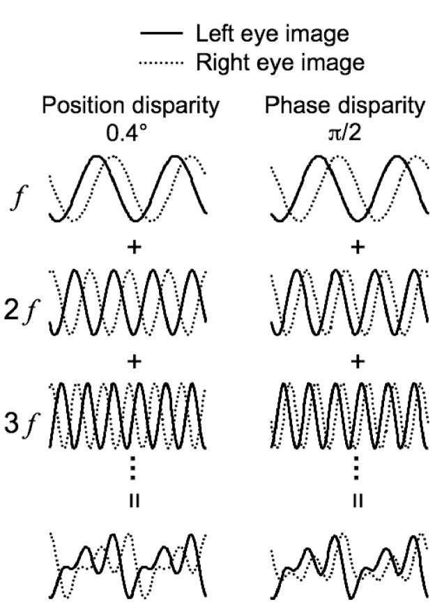
After the initial characterization of the RF, and if the neuron showed disparity selectivity to RDS, we proceeded to the main purpose of this study. We constructed the stimulus by summing 47 sinusoidal gratings with different spatial frequencies (SFs) but the same orientation. The components were a harmonic series with a fundamental frequency of 0.25 cpd, and the spatial phase of each component was set randomly and independently on each video frame. For almost all neurons in V1, this stimulus contains many components that are in the spatial passband, so the same frequency series could be used for testing all cells. Disparity was applied in two ways. A stimulus position disparity (similar to the disparities typically produced by natural viewing) was applied by shifting all the components between the eyes by a common visual angle (Figure 1A). A stimulus phase disparity was applied by shifting the phase of all the components by a common phase angle, (i.e. all components have the same interocular phase difference). Note that these phase disparities in broadband stimuli do not occur in natural vision (Haefner and Cumming, 2008). These two types of disparity can also be combined together. We tested at least 52 combinations (13 position disparities × 4 phase disparities). On some stable recordings, we completed as many as 120 combinations (15 position disparities × 8 phase disparities). We also interleaved left and right monocular images, a pair of binocularly uncorrelated compound images (the phase of each component was set independently in each eye), as well as a blank screen. In some cells, some combinations were repeated more times than other combinations in the final data, because we adjusted the combinations as we proceeded from one block to the next, to better characterize the cell.

Figure 1.

Synthesizing binocular compound images. For simplicity, only cross-sections of the images are illustrated, and only three harmonics are shown. A pair of harmonic series was built for the left (solid) and right (dotted) eyes, respectively. To create a pair of compound images with a position disparity of 0.4 deg, all the components were shifted by 0.4 deg between the eyes, and then summed. To create one with a phase disparity of π/2 rad, all the components were shifted by an interocular phase difference of π/2 rad, and then summed. Phase disparity could be combined with any position disparity. For combinations with zero phase disparity, the paired compound images were related by a translation, i.e., the binocular image had natural disparity. Other phase disparities produce image pairs that do not occur during natural binocular viewing.

The peak–to-peak contrast of images constructed in this way depends on the phase relationship of the components. In cases where the components’ peaks (or troughs) are aligned, the contrast is higher than in cases where the components’ peaks (or troughs) are evenly spread out. In order to present high contrast images, and reduce variations in overall contrast, we normalized each image so that the luminance range was as wide as permitted on our display. The peak-to-peak contrast of these images was typically 98%. On each frame, a new image was dynamically created by randomly shuffling the phase of every component in one eye. The phase of each component in the other eye was determined by the combination of this shuffled phase, position disparity, and phase disparity. The length of the square patch was equal to the fundamental period (i.e., the patch size was 4.0 × 4.0 deg), large enough that the edges of the patch were outside the minimum response field of all the cells recorded.

For our compound grating, the set of stimuli with a phase disparity of zero characterize disparity tuning in a way that is equivalent to a conventional disparity tuning curve, performed by displacing image regions between the eyes. Notice also that the set of stimuli with a phase disparity of π corresponded to a disparity-tuning curve with an anticorrelated stimulus (the two eyes images are related by a translation and contrast reversal). Despite this equivalence, these compound gratings differed from RDS in two important ways: First, a random-dot pattern is noise in 2 dimensions, while the compound grating was noise in only 1 dimension. Second, the amplitude spectrum of an RDS has random fluctuations in shape, while it was always flat in our compound gratings. Because of the differences in the image properties, it was an empirical question whether the subset of responses we find with compound gratings were directly comparable with previous studies comparing correlated and anticorrelated RDS. We therefore also tested a subset of neurons with such RDSs.

Measures for characterizing traditional tuning

The response measure used for all analyses was simply the mean firing rate over the duration of the stimulus, shifted by 50 ms to account for the response latency. One of our aims was to understand the construction of odd-symmetric disparity tuning. In order to quantify the extent to which a set of responses was even- or odd-symmetric, we calculated a symmetry index (modified from (Read and Cumming, 2004)). We denote the response (mean firing rate) to any one stimulus as r(x,φ), where x indicates the position disparity, and φ the phase disparity. The set of responses with no phase disparity, r(x,0), is equivalent to a traditional disparity tuning curve, so it is the symmetry of these data that we measured. The symmetry was defined not simply relative to 0 disparity, but relative to the center of the neuron’s response range. We estimated this using the centroid of the tuning function: x_centr = ∫ |r(x,0)− r_uncorr| · x dx / ∫ |r(x,0) − r_uncorr| dx, where r_uncorr is the response to the uncorrelated condition. The disparity tuning function was then expressed relative to this centroid, as

$$r_0(x)=r(x-x_{\text{centr}},0)-r_{\text{uncorr}}.$$ (1)

The firing rates are all expressed relative to the response to uncorrelated dots, to isolate the part of the response that is caused by disparity. This response can therefore be positive or negative, and the extent to which it is even- or odd-symmetric can be determined from the Fourier transform of r₀(x). We calculated the sum, S_evn of the cosine (even) functions across all frequency components and the sum S_odd of the sine (odd) functions. Finally, we estimated the symmetry of the tuning curve with the angular phase of the vector (S_evn, S_odd). A symmetry phase of zero indicates a function that it perfectly even symmetric about its centroid, while a symmetry phase of ±π/2 indicates a perfectly odd symmetric function. A symmetry phase of π indicates a perfectly even-symmetric response, but one that is dominated by a trough, rather than a peak.

Modeling

This study combined stimuli differing in position disparity, traditionally used to characterize tuning, with various phase disparities. Quantitative models give predictions of responses to all such stimuli. For the disparity energy model, odd-symmetry in the disparity tuning curve indicates that the left and right RFs are related by a phase disparity. When tested with combinations of position and phase disparity, such a model has a striking characteristic: the maximum response is to a stimulus containing a phase disparity that matches that of the RFs. If the monocular RFs are Gabor functions differing only in position and phase, this model predicts that the response to a set of stimulus position disparities should also be a Gabor function, described as

$$g_{\text{enrg}}(x,\phi )={\mid A·e^{-{(x-x_0)}^2/2{\sigma }^2}·cos\left\{2\pi f(x-x_0)+\nu -\phi \right\}+y_0\mid }_{+}^{\gamma }$$ (2)

where x and φ are the position disparity and the phase disparity of the stimulus, x₀ and ν are the position and phase disparity of the RF. σ and f are the standard deviation and carrier frequency of the Gabor function. The function |.|₊ is a half-wave rectifier. The function g_enrg(x,φ) reaches maximum when (x,φ.)=( x₀,ν). As the stimulus phase disparity changes, only the phase of the carrier should change, by a value equal to the change in stimulus phase disparity (Haefner and Cumming, 2008).

The second model subtracted the output of one disparity energy model from another. We call this model the two-subunit (2SU) model. Here the term “subunit” refers to the disparity-energy models that feed into the full model. The term subunit is sometimes applied to the model simple cells that feed into an energy model complex-cell, a slightly different usage. However, since all of our modeling and analyses ignore the absolute phase of the stimulus components, our “subunits” could also be simple cells (see (Haefner and Cumming, 2008) for further discussion). The two SUs in our model differed in only one parameter: x₀ (position disparity), the other six parameters were identical in the two subunits. We also added a coefficient w that represents the relative weight of the inhibitory SU. The full description of the function was therefore

$$\begin{array}{l}{g}_{\text{2SU}}(x,\phi )={\mid A·e^{-{(x-x_{0\text{exc}})}^2/2{\sigma }^2}·cos\left\{2\pi f(x-x_{0\text{exc}})+\nu -\phi \right\}+y_0\mid }_{+}^{\gamma }\\ -w·{\mid A·e^{-{(x-x_{0\text{inh}})}^2/2{\sigma }^2}·cos\left\{2\pi f(x-x_{0\text{inh}})+\nu -\phi \right\}+y_0\mid }_{+}^{\gamma }\end{array}$$ (3)

where the subscripts “exc” and “inh”, denote excitatory and inhibitory subunits respectively. Note that excitation and inhibition refer to the sign in which the outputs are combined. They do not refer to conventional classes of disparity tuning. Also, although we use only two SUs (since this is sufficient to explain the data), more than two SUs can be combined in this way.

Measures for testing model predictions

If the peak disparity is different for the two SUs, then the difference of the responses will define an odd-symmetric curve (see Figure 2). These two schemes for generating odd-symmetry (phase disparity vs 2SU) can be differentiated by examining the responses to combinations of phase and position disparity. In particular, the envelope of a set of tuning curves across all phase disparities should reveal the contributions of the two SU (see Modeling results). We estimated the upward envelope, h_up(x), simply by taking the maximum response to any phase disparity for each position disparity (and used the minimum to estimate the downward envelope h_dwn(x)):

$$\begin{array}{l}{h}_{\text{up}}(x)=\underset{\phi }{max}[r(x,\phi )-r_{\text{uncorr}}]\\ h_{\text{dwn}}(x)=\underset{\phi }{min}[r(x,\phi )-r_{\text{uncorr}}]\end{array}$$ (4)

Figure 2.

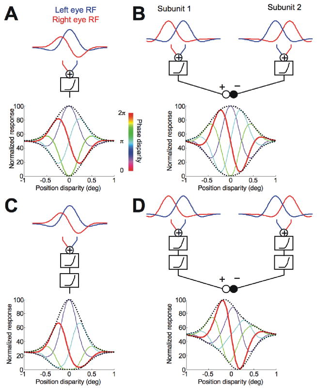
Model predictions. A, The disparity energy model of a simple cell is illustrated. The RFs had pure phase disparity. The predicted responses to a broadband compound grating are shown as a set of tuning functions for position disparity. The stimulus phase disparity is color coded (see color bar). The dashed curves indicate the envelopes. B, Two disparity energy models were linearly combined. The RFs of the subunits had pure position disparity. One subunit fed an excitatory drive and the other fed an inhibitory drive. C, The output of a disparity energy model was passed through an additional nonlinearity. The model predicts perfect symmetry of the envelope about a vertical axis. D, The outputs of the two subunits (2SU) were passed through additional nonlinearity prior to combining the signals. The 2SU model predicts an offset between the upward and downward envelopes (no symmetry about a vertical axis).

Then, the position, μ_up, and width, σ_up, for the upward envelope were given by the centroid and the standard deviation

$$\begin{array}{l}{\mu }_{\text{up}}=\int \mid h_{\text{up}}(x)\mid ·xdx/\int \mid h_{\text{up}}(x)\mid dx\\ {\sigma }_{\text{up}}^2=\int \mid h_{\text{up}}(x)\mid ·{(x-{\mu }_{\text{up}})}^{2}dx/\int \mid h_{\text{up}}(x)\mid dx\end{array}$$ (5)

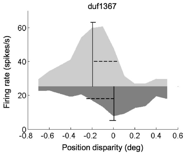
respectively. The position, μ_dwn, and width, σ_dwn, of the downward envelope were calculated similarly (Figure 4). Differences between μ_up and μ_dwn will tend to result in odd-symmetric disparity tuning. The size of this effect also depends on the envelope width, so we calculate a normalized offset:

$$\mathrm{\Delta }\mu =({\mu }_{\text{up}}-{\mu }_{\text{dwn}})/\sqrt{({\sigma }_{\text{up}}^2+{\sigma }_{\text{dwn}}^2)/2}$$ (6)

Figure 4.

Estimating offset between upward and downward envelopes. Light gray area is the upward envelope of a set of tuning curves for 8 different phase disparities. The dark gray area is the downward envelope. The boundary of the two areas is the response to an uncorrelated stimulus. The vertical solid lines indicate the estimated position (center of mass), and the horizontal dashed lines indicate the estimated width (standard deviation) of the envelopes. The small horizontal lines at the end of the vertical lines indicate the 95% confidence interval for the position estimate. This example is the same cell shown in Figure 3A.

This normalization allows tuning curves of different spatial scales to be compared. It also ensures that if an envelope is poorly defined (hence has a large s), the normalized offset is close to zero. Unless otherwise stated, all measures of envelope offset use this normalized value.

Model fitting

Although we relied on these model-free measures to characterize the basis of odd-symmetry, we needed to use model fits to explore how the 2SU model explains the effects of anticorrelation, using Equations (2) and (3). We fit the full tuning function (52–120 data points) with 7 parameters of Equation (2). Six parameters characterized the Gabor function (A, x₀, σ, f, ν, y₀), and one parameter γ implemented an output nonlinearity at the final stage with an exponent. The total number of parameters in the 2SU model of Equation (3) was nine. The functions g_enrg(x,φ) and g_2SU(x,φ) were fitted to the mean firing rate data r(x,φ). To minimize the dependence of the response variance on the response mean, we first converted the functions and the data to their square-root values (Prince et al., 2002b). Then, the summed-square errors of the functions were calculated. We searched for the parameter combination that minimized the summed-square error using fminsearch in Matlab.

Correlation coefficients with circular variables

Many of our analyses involved measuring correlations between variables, at least one of which was circular (typically a measure of phases). For the correlation between a circular variable, θ and a linear variable, x we used the circular-linear correlation R_xθ (Mardia and Jupp, 1999). It is related to Pearson’s correlation coefficient as

$$R_{x\theta }^2=\frac{{\rho }_{xc}^2+{\rho }_{xs}^2-2{\rho }_{xc}{\rho }_{xs}{\rho }_{cs}}{1-{\rho }_{cs}^2}$$ (7)

where ρ_xc=corr(x, cosθ), ρ_xs=corr(x, sinθ), and ρ_cs=corr(cosθ, sinθ). The function corr(.) denotes the Pearson’s correlation coefficient. For N observations, the value $(N-3)R_{x\theta }^2/(1-R_{x\theta }^2)$ follows an F distribution with degrees of freedom (2, N−3). In cases where the two variables are both circular, we use the circular-circular correlation

$$R_{\theta \varphi }=\frac{\sum sin({\theta }_i-\overline{\theta })·sin({\varphi }_i-\overline{\varphi })}{\sqrt{\sum {sin}^2({\theta }_i-\overline{\theta })·{sin}^2({\varphi }_i-\overline{\varphi })}}$$ (8)

where θ̄ is the angular phase of (Σcosθ_i,Σsinθ_i). For N observations, the value $\mid R_{\theta \varphi }\sqrt{N{L}_1{L}_2/L_3}\mid$ follows a two-tailed normal distribution, where L₁ = Σsin² (θ_i − θ̄)/N, L₂ = Σsin²(ϕ_i − ϕ̄)/N, and L₃ = Σ[sin²(θ_i − θ̄)·sin²(ϕ_i − ϕ̄)]N.

Results

Model predictions

In the disparity energy model, linear summation in monocular receptive fields is followed by addition and a squaring output nonlinearity (top row of Figure 2A). A phase difference between monocular RFs (“RF phase disparity”) is reflected in the phase of the disparity tuning function with no phase disparity in the stimulus (red curve in bottom row of Figure 2A). When a stimulus phase disparity was added, the phase of the disparity tuning function shifted accordingly. Previous studies of disparity selectivity have used stimuli equivalent to our condition with zero phase disparity, where the images in the left and right eyes are related by a simple translation. This resembles the disparities produced by natural viewing conditions. Stimulus phase disparities in broadband images are not produced by natural viewing, and we refer to these as unnatural disparities. The peak response across all conditions occurred when both the stimulus phase disparity matched the RF phase disparity and the stimulus position disparity matched the RF position disparity (peak of the purple curve in bottom row of Figure 2A). For a stimulus phase disparity of π (anticorrelation), the tuning curve was inverted (cyan curve in bottom row of Figure 2A). The dotted lines in Figure 2A show the envelope encompassing all responses. If the model had a different RF phase disparity, the curves in Figure 2A would be associated with a shifted value of stimulus phase disparity. That is, the colors of the individual lines would change, but the envelope of the responses is unaffected. Note that these envelopes were symmetrical both about a horizontal axis and a vertical axis. The width of the envelope reflects the envelope of the monocular RFs.

Linearly combining two disparity energy models, which differ only in RF position disparity, produced results very similar to the disparity energy model, with an envelope that is symmetrical about both vertical and horizontal axes. Note that the energy model simulation in Figure 2A produced odd symmetry by means of a phase disparity, while the odd symmetry in Figure 2B was produced by two subunits, each of which had an even symmetric response to disparity.

Incorporating an additional output nonlinearity at the final stage of the energy model produced a characteristic pattern (Figure 2C). The nonlinearity accentuated the peak response, and hence broke the symmetry of the standard model about the horizontal axis. This kind of asymmetry in the envelope provides a simple way to estimate the output nonlinearity required to best describe real neuronal responses with the energy model. The symmetry of the envelope about a vertical axis was preserved. Consequently, it remained true that the peak response occurred when the stimulus contained a phase disparity matching that of the RFs, and the envelope peak still identified the RF position disparity. Note that the model in Figure 2A was just a special case of this general model, with a final output exponent of one.

The additional output exponent changed the shape of the disparity-tuning curve (red line), so that although the RF phase disparity was p/2, the tuning curve was no longer exactly odd-symmetric. Thus attempts to infer phase disparity from the shape of the disparity tuning of real cells will have systematic errors that depend upon the output nonlinearity. Our manipulation of phase disparity in the stimulus allowed us to identify the RF phase disparity in a way that is not affected by any output nonlinearity, because the stimulus phase disparity that matched the RF phase disparity elicited the highest response in all cases.

In the final model (Figure 2D), we used the same two subunits as shown in Figure 2B, but passed the output of each through the same expansive nonlinearity, prior to combining the two signals. The individual subunits responded maximally to certain position disparities. This property of the subunits derives from their RF position disparities. As phase disparity was added to the stimulus, the amplitude of the tuning curve of each subunit is reduced. The additional nonlinearity is responsible for this reduction, so that in each subunit, the response magnitude for anticorrelated stimuli is lower than for correlated stimuli. This remains true after subtracting the output of one subunit from the other. The combined response to correlated stimuli is odd symmetric, because the response of the added subunit dominates at near disparities, while the response of the subtracted subunit dominates at far disparities. This broke the symmetry around the vertical axis seen in the other three models. The overall positive peak of the upward envelope roughly corresponds to the position disparity of one subunit, while the minimum in the downward envelope corresponds to the position disparity of the second subunit. This lack of symmetry about a vertical axis cannot be produced by variants of just a single energy model. Thus, envelope asymmetry about a vertical axis provides an empirical signature of contributions from more than one subunit.

The responses to natural disparities (zero stimulus phase disparity, red curve) are very similar in Figure 2A-D. It is only by comparing responses across a range of stimulus phase disparities that the difference between the two mechanisms becomes apparent. This comparison yields four important pieces of information. First, the effect of an output exponent can clearly be visualized because of a difference in the size of upward and downward envelopes (Figure 2C). Second, for the energy model, the stimulus phase disparity that produces the maximum response matches the RF phase disparity, regardless of any output nonlinearity. Third, even for a 2SU model, the optimal stimulus phase disparity is close to the RF phase disparity of the excitatory subunit (a measurement that is not affected by the output nonlinearity). Fourth, the positions of the extrema in the envelope lie close to the position disparities of the two SUs. The last point is informative only if the SUs’ RF position disparities are offset. Otherwise, the test cannot differentiate the 2SU mechanism from a single energy mechanism. The number of detected 2SU mechanisms in the population of recorded cells therefore provides only a lower limit of the true number.

Neuronal Data

We recorded from 116 cells in V1 and 121 cells in V2 (this is not an unbiased sample –many cells that did not show evidence of disparity selectivity in our initial screening using an RDS are not included in these figures). We selected cells for this study based on three criteria. First, the median number of repetitions across all the combinations of position disparity and phase disparity had to be at least eight (mean 20 for the analyzed cells). Second, the maximum of the mean firing rates across all combinations had to be larger than 10 spikes/s. Third, the square-root of the firing rates across all conditions had to show a significant effect of disparity condition (one way ANOVA, p < 0.01). Sixty seven cells from V1 and 66 cells from V2 met these criteria. In a small number of cells, the modulation was sufficiently weak that no systematic relationship was clear between responses for the two different kinds of disparity. We therefore also required a significant interaction between position disparity and phase disparity on a 2-way ANOVA (p < 0.01), which left us with a sample of 64 cells from V1 (duf 37; ruf 27) and 61 cells from V2 (duf 30; ruf 31). Note that the recording chamber allowed us access to large regions of V1 on the operculum that did not lie over V2. This allowed us to collect data from neurons in V1 and V2 with RFs over similar eccentricity ranges (mean 5.2 deg, SD 1.3 deg in V1; mean 4.9 deg, SD 1.3 deg in V2);

Example cells

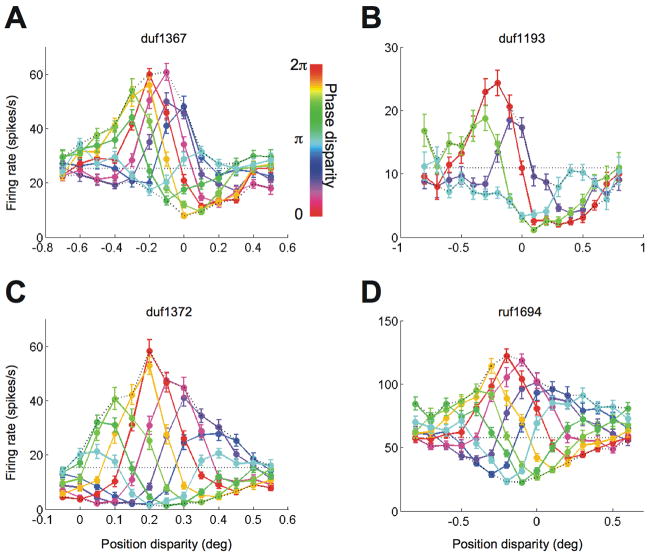
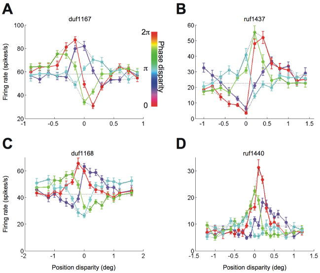
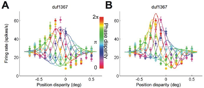
Figure 3A and B show the responses of V1 cells with substantial odd-symmetric components in the disparity tuning for a phase disparity of zero (red curves). Looking at the responses across all conditions, it is clear that the upward envelope peaks at a different disparity from the downward envelope. Figure 4 illustrates how this shift was quantified, by calculating the centroid for each half of the envelope. The significance of any envelope offset was determined by bootstrap resampling, and was highly significant for the examples in Figure 3A and B (p< 0.001). Thus these two neurons show clear evidence of contributions from more than one energy-model SU.

Figure 3.

Example cells from V1. A and B, Two cells are shown with an odd-symmetric component in the tuning for natural disparity (red curve). Position disparity and phase disparity were combined in the stimulus. The abscissa indicates the position disparity, and the line-color indicates the phase disparity. The upward envelopes were offset from the downward envelopes. The error-bars indicate standard error. C and D, Two cells are shown with mostly even-symmetric tuning for natural disparity. The envelopes showed no offset (D) or a poorly defined offset (C).

Figure 3C and D show the responses of two V1 neurons with responses to natural disparity (red curve) that are nearly even symmetrical. Figure 3D shows an example that is nearly symmetrical about both vertical and horizontal axes, behaving almost exactly as predicted by the energy model. Figure 3C shows an example where the effect of an additional output exponent (or a thresholding) is clearly visible. This is so marked that the downward envelope is poorly defined, and it is difficult to know whether there is an offset between the upward and downward envelopes. Consequently these data are compatible with an energy model with additional threshold. Because our measurement of the envelope offset takes in to account the width of the envelope (see Methods), the offset for these data is small, and was not significant on resampling (p > 0.05). It is important to note that these two examples of neurons that are well described by an energy model could equally well be described by a 2SU model, but there is no feature in the data that requires us to invoke the 2SU model.

Cells recorded in V2 shared many of their features with the cells in V1. For example, V2 cells with an odd-symmetric disparity tuning to natural disparities had envelopes that were offset (Figure 5A and B). The V2 cells had stronger odd-symmetric components and had clearer offsets than the V1 cells shown in Figure 3A and B. We also found V2 cells with even-symmetric disparity tuning. The envelopes of some these cells were symmetrical about a horizontal axis (Figure 5C, closely matching the energy model), while the downward envelopes of other cells were greatly compressed (Figure 5D). Although the features relevant for testing the underlying mechanism were qualitatively similar between the two areas, note that the range of disparities spanned by the responses was larger in the V2 cells than in the V1 cells. This can be seen in the different scales of the abscissa between Figure 3 and Figure 5.

Figure 5.

Example cells from V2. A and B, Two cells are shown with a strong odd-symmetric component in the tuning for natural disparity. The upward envelope was offset from the downward envelope. Plotting conventions are the same as in Figure 3. C and D, Two cells are shown with mostly even-symmetric tuning for natural disparity. The envelopes were not offset or not well defined.

Population data

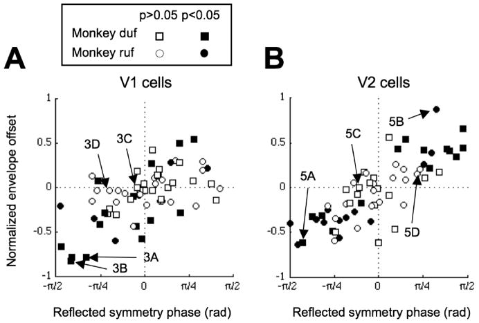
If combining inputs from more than one subunit plays an important role in the generation of odd-symmetric disparity tuning, then there should be a systematic relationship between two of our measures: the envelope offset (which combines information from all stimulus phase disparities), and the symmetry phase of responses to stimuli with zero phase disparity. The relationship between the two variables in V1 neurons is shown in Figure 6A, where there is a strong correlation (R_xθ=0.63, p=7.2×10⁻¹²). In this plot, values of symmetry phase less than −π/2 are reflected about −π/2, so that perfect even symmetry (symmetry phase of 0 or π) is plotted in the center, while perfect odd symmetry is plotted at the left (for “near” cells) or right (“far” cells) extreme of the abscissa. In the 2SU model, cells with a strong odd-symmetric component in the disparity tuning should have a large offset between the upward and downward envelopes, in the appropriate direction. This yields points in either the upper right or lower left quadrants. (Note that they need not lie along the identity line. Exactly where model neurons fall depends on several of the model parameters, such as the output nonlinearity). Energy model neurons should all lie along the horizontal axis, with zero envelope offset. A third (21/64) of the V1 cells had significant envelope offsets, and only 2/21 of these fell in the wrong quadrants. Note that for neurons with even symmetric tuning curves, even if there were multiple subunits, this need not result in an envelope offset. So the fraction of neurons showing significant offsets is a lower bound on the fraction that is constructed from two or more subunits. The remaining V1 cells lay close to the horizontal line in agreement with the energy model.

Figure 6.

Relationship between symmetry phase and envelope offset. A, The offset was correlated with the symmetry in the V1 population. The symmetry phase was reflected at ±π/2, so that odd-symmetry increased monotonically towards the ends of the abscissa. The offset of the envelope was normalized by the width. The shape of the symbols indicates monkey identity. The filled symbols represent cells with significant envelope offsets (Bootstrap resampling, p<0.05). Labeled arrows indicate the example cells shown in Figure 3. B, The offset was strongly correlated with the symmetry in the V2 population. All the cells with significant offsets lay in the correct quadrant predicted by the 2SU model. Labeled arrows indicate the example cells shown in Figure 5.

In V2, there was a strong correlation between the reflected symmetry phase and the normalized offset (R_xθ=0.80, p=0; Figure 6B). The correlation was significantly stronger than we saw in V1 (p=0.020). Of the 61 V2 cells, 27 (44%) showed significant envelope offsets. Furthermore, all of the neurons with significant offsets fell in the predicted quadrants. V2 also shows fewer neurons with odd symmetry but little envelope offset –that is fewer cells where a single energy model using phase disparity can account for the data. All of these features can be explained by suggesting that the increase in odd symmetry in V2 (more values of reflected symmetry phase close to ±p/2), is in part explained by combining inputs from V1 that have different position disparities.

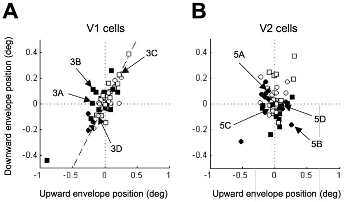
The demonstration of significant envelope offsets in both V1 and V2 provides statistical evidence that the traditional energy model does not completely capture the responses of these neurons. Some insight into the magnitude of these deviations can be gained by comparing the upward and downward envelope positions for each cell. In the energy model, the two envelope positions coincide (Figure 2), so these data should lie along the identity line. The data from V1 lie close to the identity line (r_S=0.65, p=1.3×10⁻⁸; Figure 7A), indicating a good deal of agreement with the energy model. In contrast, the upward and downward envelopes of the V2 cells were uncorrelated (r_S=− 0.07, p=0.60; Figure 7B). The difference between the correlation coefficients for V1 and V2 was highly significant (p=1.9×10⁻⁶). Thus these deviations from the energy model are substantially larger in V2 than in V1.

Figure 7.

Relationship between the positions of the upward and downward envelopes. A, In the V1 population, the two positions were highly correlated. The points lay close to the identity line (dashed), in broad agreement with the energy model. The positions of the envelopes were not normalized by their widths. The filled symbols represent cells with significant offsets as in Figure 6 (Bootstrap resampling, p<0.05). B, In the V2 population, the two positions were not correlated, indicating much larger deviations from the energy model.

An important feature of Figure 7 is that the marginal distributions of envelope positions were similar in V1 and V2, both for upward (mean 0.01±0.17° in V1; 0.01± 0.14° in V2) and downward envelopes (mean 0.02±0.12° for V1; 0.02±0.12° for V2). However, because of the different correlation, the scatter in the difference between trough and peak locations was significantly larger for V2 than for V1 (SD 0.10 in V1, SD 0.17 in V2; F-test, p=10⁻⁴). All of these features follow if the output of V1 neurons (themselves close to the energy model) with different position disparities are combined to generate odd symmetry in V2 neurons. This could also provide a mechanism by which the overall range spanned by individual disparity tuning curves in V2 might be wider than in V1 (Poggio et al., 1988), explaining observed differences in “disparity frequency” (Cumming and DeAngelis, 2001; Parker, 2007).

Phase disparity of RFs

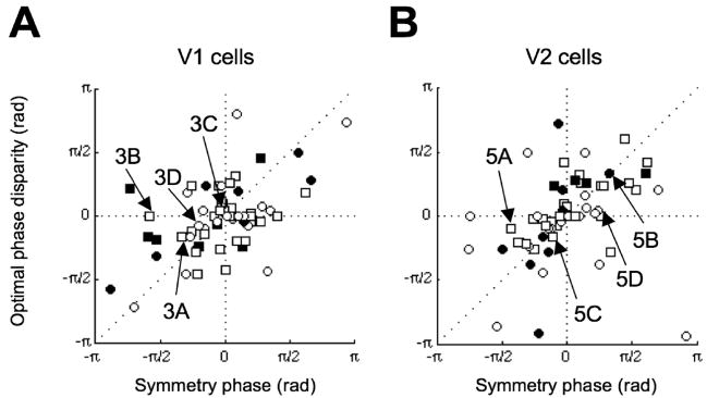
The 2SU model provides a scheme in which it is possible to describe the form of responses to natural disparity without invoking phase disparity, because differences in position disparity between the subunits can generate tuning curves with a range of shapes. Our data indicate that such a mechanism plays an important role in V1 and in V2. This does not imply that phase disparity plays no role. It is possible that the subunits themselves (constructed with the traditional disparity energy model) contain phase disparities. One of the advantages of the new stimulus we describe (with many spatial components, unlike (Haefner and Cumming, 2008)), is that a phase disparity within the subunits has a measurable effect on the tuning. A striking feature of the energy model is that the largest response across all conditions occurs in the presence of a stimulus phase disparity (see Figure 5B) that matches the RF phase disparity. If the subunits used in the 2SU model have phase disparity, again the largest overall response will occur when the stimulus has this phase disparity. Thus, simply estimating the stimulus phase disparity associated with the largest overall response provides a model free way to demonstrate RF phase disparity, even for the 2SU model. For each phase disparity, we found the largest response, r_peak(φ), elicited across position disparity. We then used spline interpolation to estimate the phase disparity producing the largest response. We ensured that the interpolated function had properties of a real periodic function, i.e. the two ends connect smoothly. This analysis of our full data set allows phase disparity to be estimated directly, regardless of the symmetry in disparity tuning. In order to examine whether these phase disparities also play a systematic role in determining the shape of the disparity-tuning curve, we examined the relationship between symmetry phase and the optimal stimulus phase disparity. The significant correlation between these values in V1 (R_θϕ=0.35, p=0.01; Figure 8A) indicates that phase disparity does indeed play a significant role in constructing odd-symmetric disparity selectivity. In fact, 14/64 (22%) of the cells had an optimal phase disparity significantly deviated from zero (Bootstrap resampling, p<0.05). Neurons from V2 showed a similar pattern (R_θϕ=0.58, p=7.0×10⁻⁴), with 13/61 (21%) of the cells having significant phase disparities (Bootstrap resampling, p<0.05; Figure 8B). These results support earlier studies suggesting that a component of odd-symmetry in the disparity tuning of both simple and complex cells can be explained by phase disparity in the RFs. Importantly, the range of optimal stimulus phase disparities is similar in V1 and V2. This suggests that these RF phase disparities could be inherited from disparity-selective neurons in V1, without the need to combine monocular inputs from scratch in V2. These phase disparities in V2 are correlated with the envelope offset (R_xθ=0.51, p =2.0×10⁻⁶), suggesting that the two mechanisms work together to produce odd symmetry. In V1, these two measures were not significantly correlated (R_xθ=0.18, p = 0.13).

Figure 8.

Relationship between symmetry phase and optimal phase disparity. A, The optimal phase disparity (stimulus phase disparity producing the maximum spike rate) was correlated with the symmetry phase in the V1 population. The standard energy model predicts points that lie along the diagonal. Filled symbols represent cells with significant optimal phase disparity (Bootstrap resampling, p<0.05). The shape of the symbols indicates monkey identity. B, A similar correlation was found in the V2 population. Cells in both V1 and V2 seem to use RF phase disparity to build odd-symmetric tuning. Note that in this plot (unlike Figure 6), the symmetry phase is not reflected at ±π/2. Since both variables are circular, the full range can be used.

This demonstration of RF phase disparity is unsurprising for V1 simple cells, where phase disparity can be clearly demonstrated by comparing monocular receptive field maps (Freeman and Ohzawa, 1990; Anzai et al., 1999a). But for complex cells, especially cells in extrastriate cortex, the evidence that phase disparity plays a role has been much more indirect, based upon the shape of the response to disparity (Ohzawa et al., 1997; Anzai et al., 1999c; Prince et al., 2002a; DeAngelis and Uka, 2003). We classified cells as simple or complex on the basis of the modulation (F1/F0 ratio (Skottun et al., 1991)) in firing rate to a monocular grating at the preferred orientation and spatial frequency. The distribution of phase disparities was similar in simple and complex cells. Thus this result produces the strongest evidence to date that phase disparity plays an important role in shaping the disparity selectivity of complex cells.

Previous studies of phase disparity in the cat reported a relationship between phase disparity and orientation. In simple cells, neurons with vertically oriented RFs tend to have a wider range of phase disparity (DeAngelis et al., 1991; Ohzawa et al., 1996; Anzai et al., 1999b). In complex cells a weak correlation was observed in the opposite direction (Ohzawa et al., 1997; Anzai et al., 1999c). However, the complex cell studies inferred phase disparity from the symmetry of the disparity response. Using our more direct measure (the optimal stimulus phase disparity), we found no evidence that cells preferring horizontal orientation (within 20 deg of horizontal) have less phase disparity than cells preferring vertical orientation (within 20 deg of vertical) in either V1 or V2 (F-test p=0.12 for V1 and p=0.27 for V2). We also saw no differences when looking at simple or complex cells separately.

Attenuated tuning for anticorrelated stimuli

The 2SU model, like neurons in V1 and V2, exhibited an attenuated disparity tuning for a phase disparity of π compared to the disparity tuning for a phase disparity of zero. Notice that when a phase disparity of π is applied to our compound grating, the result is an anticorrelated stereogram, so this result replicates earlier studies using RDSs (Cumming and Parker, 1997) and bars (Ohzawa et al., 1990; Ohzawa, 1998). Even the energy model, with a final output exponent, can produce some such attenuation (Lippert and Wagner, 2001), at least for tuning curves that are not odd-symmetric (Read et al., 2002). The 2SU model allows a much wider range of tuning curves and attenuation magnitudes to be explained. In order to examine whether the 2SU model accounts for the observed effects of anticorrelation, we fit the energy model and the 2SU model to the entire data set for each cell (an example is shown in Figure 9), and examined the fitted responses to anticorrelation. This is the first data analysis to use Equations (2) and (3) in their explicit forms. For the energy model fits, the amplitude ratio (median 0.86 in V1 and median 0.93 in V2) is significantly larger than for the fits with the 2SU model (median 0.41 in V1, difference Wilcoxon test p=1.2 × 10⁻⁶; median 0.40 in V2, difference Wilcoxon test p=1.7×10⁻⁷). We compared these model results to a purely descriptive measure of the attenuation based on fitting Gabor functions of different amplitudes to the correlated and anticorrelated data, with no constraints on the fitted amplitude ratio (Cumming and Parker, 1997; Haefner and Cumming, 2008). The ratio estimated this way (median 0.44 in V1, 0.41 in V2), is very similar to that produced by the 2SU fits (0.41 and 0.40 respectively, neither different by Wilcoxon test). This suggests that the summation of two energy-model-like subunits provides an adequate explanation for the observed response attenuation for anticorrelated stimuli.

Figure 9.

Fitting a set of tuning curves with two different models. A, The energy model fit failed to capture important features of the data from an example V1 cell. C, The 2SU model provided a good fit to the same example cell.

Note that the effects of anticorrelation on neuronal responses are similar in both areas, and the 2SU model fits these better than the energy model. The similarity between V1 and V2 may seem surprising given the differences we demonstrate between V1 and V2 above. However, the primary difference is that V2 neurons appear to have larger differences in position disparity between subunits. This need not have a substantial impact on responses to anticorrelation – it is possible that the attenuated responses to anticorrelation in V1 neurons are produced by summing two subunits, but with similar position disparities.

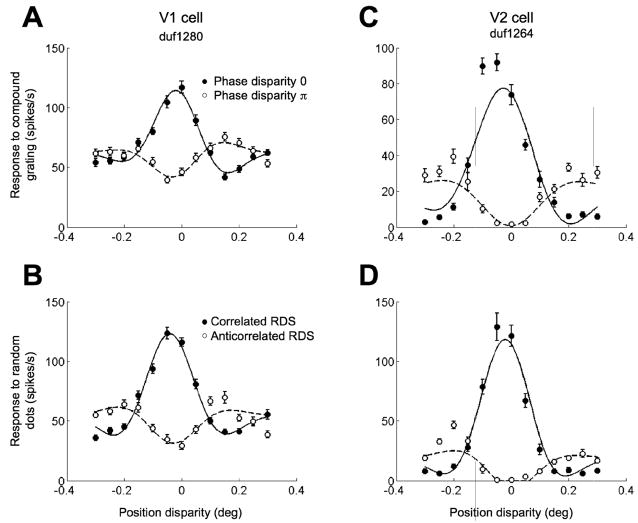
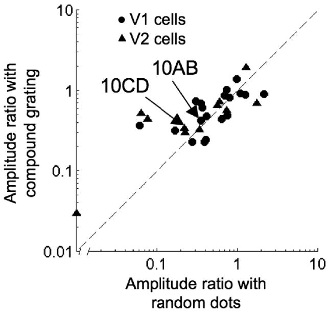
These conclusions depend on the assumption that attenuation observed using these compound gratings is similar to that observed with RDS. We were able to examine this in a subset of neurons for which we obtained responses with both RDS and compound gratings. Many cases showed strikingly similar responses (Figure 10), and the amplitude ratio for RDS was very similar to that for compound gratings both in V1 (r_S=0.73, p=0.006, n=19) and in V2 (r_S=0.76, p=0.009, n=11; Figure 11). Thus, the 2SU mechanism can explain the effect of anticorrelation in both RDS and compound gratings. Interestingly, a similar comparison of RDS with compound gratings containing only 2 components found that attenuation in the compound gratings was significantly smaller (Haefner and Cumming, 2008). This suggests that including a range of frequency components improves the characterization of the two subunits.

Figure 10.

Similarity with responses to correlated and anticorrelated random-dot stereograms (RDSs). A, From the various combinations of position disparity and phase disparity of a compound image, the disparity combinations with a phase disparity of zero or of π were extracted from the data of an example V1 cell. The smooth curves are Gabor functions fitted to the data. The two functions shared all their parameters, but the amplitude and the phase. B, The neuron produces very similar responses to binocularly correlated and anticorrelated RDSs. C, Same as in A, but a cell recorded in V2. D, This V2 cell exhibited higher responses to an RDS otherwise the pattern of results is very similar.

Figure 11.

Similar attenuation of responses to anticorrelated stimuli across the two image classes. For each stimulus class (i.e., compound gratings and random dots), we calculated the ratio of disparity tuning amplitude with anticorrelated stimuli over the amplitude with correlated stimuli. No difference was observed in the ratio between the image classes, in either V1 or V2.

Discussion

We describe the effects of a new kind of disparity manipulation on the activity of disparity-selective neurons in areas V1 and V2. This manipulation involves applying the same interocular phase shift to all of the Fourier components of an image (stimulus phase disparity). When combined with traditional disparity (stimulus position disparity) this reveals new features of the mechanism by which signals about disparity are constructed in V1 and V2. First it confirms the predictions of a new model (Haefner and Cumming, 2008) suggesting that the responses of many neurons (about one third), represent the summation of responses from 2 (or more) subunits that behave like the disparity energy model (the 2SU model). Second, these subunits are more strongly related to the presence of odd-symmetry in V2 than in V1, presumably reflecting a systematic transformation in the projection from V1 to V2. Third, we show that phase disparities are present within the subunits, and these phase disparities also play an important role in generating odd-symmetric tuning, both in V1 and in V2. This is the first demonstration that phase disparities are represented in the extrastriate cortex.

The geometry of binocular projection means that small areas of the image are very similar in the two eyes, up to a translation – i.e. it produces stimulus position disparities. The 2SU model was originally developed to explain how neurons are able to dedicate their dynamic range to these naturally occurring disparities (Haefner and Cumming, 2008), and the distinction was demonstrated in responses to gratings with just two frequency components. However, for any given pair of spatial frequencies, situations might occasionally occur where by chance two frequencies exhibit the same interocular phase difference. Contrastingly, situations in which many frequency components all share the same phase disparity are vanishingly rare (hence we refer to these as “unnatural”). For this reason, the observation (Figure 8) that many neurons show their strongest response to stimuli with such phase disparity in our broadband stimulus, and the correlation between this phase disparity and odd-symmetric tuning, is a powerful vindication the role of phase disparity. For V1 complex cells, and for cells in extrastriate cortex, this is the most direct evidence to date for a role of phase disparity. Haefner and Cumming did not rule out a contribution from phase disparities.

In addition to demonstrating the importance of RF phase disparity, these data also demonstrate the operation of an additional mechanism (as suggested by (Haefner and Cumming, 2008)) that generates odd-symmetric disparity tuning: combining the outputs of two energy model neurons that have different position disparities. The fact that the envelope of all responses is not symmetrical around a vertical axis (illustrated in Figure 2) is a distinctive prediction of the 2SU model, and is one that can be seen directly in such plots. In the past, a number of modifications to the energy model have been proposed to account for quantitative discrepancies with real data, including modified output nonlinearities (Lippert and Wagner, 2001), normalization (Ohzawa et al., 1997), and nonlinearities before binocular summation (Read et al., 2002). None of these previous suggestions accounts for the pattern of results demonstrated here. Indeed, it is hard to see how any model using just one pair of binocular filters in quadrature could explain this kind of asymmetry. Thus these new data provide powerful support for the 2SU model of Haefner and Cumming (2008), who only explored responses to gratings with two components. We show here that this model makes a distinctive prediction about responses to broadband patterns, and that neurons in V1 and V2 behave as predicted.

If the two subunits do not have phase disparities, the entire dynamic range of a 2SU model is spanned by naturally occurring disparities. This may be one reason why the 2SU mechanism is employed by real neurons (Haefner and Cumming, 2008). The model achieves this in two stages. In the first stage, nonlinearity at the output of a traditional energy model enhances the peak responses. If this peak response occurs for a pure position disparity, the resulting enhancement for natural disparities is greater than suppression by unnatural disparities. In the second stage, the response of a second such unit, with a different peak location, is subtracted. The result is that both extrema now occur for natural disparities. This subtraction is similar to summation of two subunits, provided the second subunit produces a pronounced minimum response for some natural disparity. Such responses are characteristic of the “Tuned Inhibitory” cells, that are uncommon outside V1. This suggests that one important function of Tuned Inhibitory neurons is that they form building blocks for odd-symmetric disparity tuning curves early in the visual hierarchy.

Because the 2SU model explains how the dynamic range is concentrated on naturally occurring disparities, it can also explain why a related manipulation – anticorrelation –reduces response magnitudes in disparity selective neurons (Cumming and Parker, 1997; Ohzawa, 1998). In anticorrelated RDS one eyes’ image is contrast reversed. This corresponds to applying a stimulus phase disparity of p. When this manipulation was explored in compound gratings with only two components, the attenuation observed was systematically weaker than that observed for RDS (Haefner and Cumming, 2008). Here we show that in a compound grating with many components, the attenuation observed is very similar to that in response to RDS. This increase in attenuation as spatial components are added is predicted by the 2SU model. Importantly, the good agreement we find between attenuation for RDS and compound gratings is not inevitable, as there are two important differences between these two stimuli. First, the compound grating is a one-dimensional noise pattern while RDS are two-dimensional. Perceptually, anticorrelation is more disruptive in 2D noise than in 1D noise (Read and Eagle, 2000). That these stimuli have similar effects in early visual cortex reinforces the view that processing downstream of V1/V2 is required to explain the perceptual effects of anticorrelation (Janssen et al., 2003). Second, RDS patterns have random variation in the power at individual spatial frequencies (even though on average the spectrum is flat), while our compound gratings have flat power spectra in every frame. These fluctuations do not play an important role in the attenuation produced by anticorrelation.

In the case of extrastriate cortex, the use of a 2SU model seems natural – it is easy to imagine that several disparity selective neurons from V1 converge onto a single disparity selective neuron in V2. If those V1 afferents have different position disparities, this provides a mechanism for generating odd-symmetric disparity tuning in area V2. The strong relationship between our estimate of subunit offset and the degree of odd-symmetry in V2 (Figure 6) indicates that such a mechanism does indeed play an important role. It seems likely that a similar mechanism in subsequent projections contributes to the increasing tendency towards odd-symmetric tuning as the visual hierarchy is ascended (Cumming and DeAngelis, 2001).

The same proposal, that V2 neurons receive input from V1 neurons with different disparity selectivity, accounts for another property of V2 neurons -- their response to edges defined only by disparity in RDS (von der Heydt et al., 2000; Bredfeldt and Cumming, 2006). The model proposed by Bredfeldt and Cumming (2006) requires in addition that the RF locations of the V1 inputs differ somewhat. Note, that since the disparity applied in the current study was uniform over a region of 4°×4°, the RF displacements proposed by Bredfeldt and Cumming (2006) would not have altered the observations we report here. Consequently, a single model in which V2 neurons receive input from at least two V1 neurons, that differ both in their disparity selectivity and their RF location, is able to explain all of the data presented here and the data of Bredfeldt and Cumming (2006). Combining inputs from V1 subunits with different disparity preferences has also been used to explain differences between V1 and V2 in signaling relative disparity (Thomas et al., 2002). Once again, it seems plausible that a similar process occurs in subsequent projections, and this might explain how responses to more complex surfaces are generated in MT (Nguyenkim and DeAngelis, 2003) or IT (Janssen et al., 2001).

The energy model provides a simple account of many properties of initial disparity coding. Phase disparities of RFs make cells maximally responsive to unnatural stimuli, a striking property that we demonstrated in some V1 and V2 neurons. Although these signals may serve useful functions when determining stereo correspondence (Read and Cumming, 2007), it seems wasteful to replicate these signals higher in the visual pathway. We showed that in V1, and particularly in V2, signals from neurons with different RF position disparities are combined to produce odd-symmetric tuning by a mechanism different from RF phase disparity. This mechanism ensures that each cell devotes more of its dynamic range to signaling naturally occurring stimuli. The manipulation we described can be applied to any image, and so can readily be adapted to see if this is a general property of projections in the extrastriate cortex.

References

- Anzai A, Ohzawa I, Freeman RD. Neural mechanisms for encoding binocular disparity: receptive field position versus phase. J Neurophysiol. 1999a;82:874–890. doi: 10.1152/jn.1999.82.2.874. [DOI] [PubMed] [Google Scholar]
- Anzai A, Ohzawa I, Freeman RD. Neural mechanisms for processing binocular information I. Simple cells. J Neurophysiol. 1999b;82:891–908. doi: 10.1152/jn.1999.82.2.891. [DOI] [PubMed] [Google Scholar]
- Anzai A, Ohzawa I, Freeman RD. Neural mechanisms for processing binocular information II. Complex cells J Neurophysiol. 1999c;82:909–924. doi: 10.1152/jn.1999.82.2.909. [DOI] [PubMed] [Google Scholar]
- Bredfeldt CE, Cumming BG. A simple account of cyclopean edge responses in macaque V2. J Neurosci. 2006;26:7581–7596. doi: 10.1523/JNEUROSCI.5308-05.2006. [DOI] [PMC free article] [PubMed] [Google Scholar]
- Cumming BG, DeAngelis GC. The physiology of stereopsis. Annu Rev Neurosci. 2001;24:203–238. doi: 10.1146/annurev.neuro.24.1.203. [DOI] [PubMed] [Google Scholar]
- Cumming BG, Parker AJ. Responses of primary visual cortical neurons to binocular disparity without depth perception. Nature. 1997;389:280–283. doi: 10.1038/38487. [DOI] [PubMed] [Google Scholar]
- Cumming BG, Parker AJ. Binocular neurons in V1 of awake monkeys are selective for absolute, not relative, disparity. J Neurosci. 1999;19:5602–5618. doi: 10.1523/JNEUROSCI.19-13-05602.1999. [DOI] [PMC free article] [PubMed] [Google Scholar]
- DeAngelis GC, Ohzawa I, Freeman RD. Depth is encoded in the visual cortex by a specialized receptive field structure. Nature. 1991;352:156–159. doi: 10.1038/352156a0. [DOI] [PubMed] [Google Scholar]
- DeAngelis GC, Uka T. Coding of horizontal disparity and velocity by MT neurons in the alert macaque. J Neurophysiol. 2003;89:1094–1111. doi: 10.1152/jn.00717.2002. [DOI] [PubMed] [Google Scholar]
- Freeman RD, Ohzawa I. On the neurophysiological organization of binocular vision. Vision Res. 1990;30:1661–1676. doi: 10.1016/0042-6989(90)90151-a. [DOI] [PubMed] [Google Scholar]
- Haefner RM, Cumming BG. Adaptation to natural binocular disparities in primate V1 explained by a generalized energy model. Neuron. 2008;57:147–158. doi: 10.1016/j.neuron.2007.10.042. [DOI] [PMC free article] [PubMed] [Google Scholar]
- Janssen P, Vogels R, Liu Y, Orban GA. Macaque inferior temporal neurons are selective for three-dimensional boundaries and surfaces. J Neurosci. 2001;21:9419–9429. doi: 10.1523/JNEUROSCI.21-23-09419.2001. [DOI] [PMC free article] [PubMed] [Google Scholar]
- Janssen P, Vogels R, Liu Y, Orban GA. At least at the level of inferior temporal cortex, the stereo correspondence problem is solved. Neuron. 2003;37:693–701. doi: 10.1016/s0896-6273(03)00023-0. [DOI] [PubMed] [Google Scholar]
- Lippert J, Wagner H. A threshold explains modulation of neural responses to opposite-contrast stereograms. Neuroreport. 2001;12:3205–3208. doi: 10.1097/00001756-200110290-00013. [DOI] [PubMed] [Google Scholar]
- Mardia KV, Jupp PE. Directional Statistics (Wiley Series in Probability and Statistics) Wiley; Chichester: 1999. [Google Scholar]
- Nguyenkim JD, DeAngelis GC. Disparity-based coding of three-dimensional surface orientation by macaque middle temporal neurons. J Neurosci. 2003;23:7117–7128. doi: 10.1523/JNEUROSCI.23-18-07117.2003. [DOI] [PMC free article] [PubMed] [Google Scholar]
- Ohzawa I. Mechanisms of stereoscopic vision: the disparity energy model. Curr Opin Neurobiol. 1998;8:509–515. doi: 10.1016/s0959-4388(98)80039-1. [DOI] [PubMed] [Google Scholar]
- Ohzawa I, DeAngelis GC, Freeman RD. Stereoscopic depth discrimination in the visual cortex: neurons ideally suited as disparity detectors. Science. 1990;249:1037–1041. doi: 10.1126/science.2396096. [DOI] [PubMed] [Google Scholar]
- Ohzawa I, DeAngelis GC, Freeman RD. Encoding of binocular disparity by simple cells in the cat’s visual cortex. J Neurophysiol. 1996;75:1779–1805. doi: 10.1152/jn.1996.75.5.1779. [DOI] [PubMed] [Google Scholar]
- Ohzawa I, DeAngelis GC, Freeman RD. Encoding of binocular disparity by complex cells in the cat’s visual cortex. J Neurophysiol. 1997;77:2879–2909. doi: 10.1152/jn.1997.77.6.2879. [DOI] [PubMed] [Google Scholar]
- Parker AJ. Binocular depth perception and the cerebral cortex. Nat Rev Neurosci. 2007;8:379–391. doi: 10.1038/nrn2131. [DOI] [PubMed] [Google Scholar]
- Poggio GF, Gonzalez F, Krause F. Stereoscopic mechanisms in monkey visual cortex: binocular correlation and disparity selectivity. J Neurosci. 1988;8:4531–4550. doi: 10.1523/JNEUROSCI.08-12-04531.1988. [DOI] [PMC free article] [PubMed] [Google Scholar]
- Prince SJ, Cumming BG, Parker AJ. Range and mechanism of encoding of horizontal disparity in macaque V1. J Neurophysiol. 2002a;87:209–221. doi: 10.1152/jn.00466.2000. [DOI] [PubMed] [Google Scholar]
- Prince SJ, Pointon AD, Cumming BG, Parker AJ. Quantitative analysis of the responses of V1 neurons to horizontal disparity in dynamic random-dot stereograms. J Neurophysiol. 2002b;87:191–208. doi: 10.1152/jn.00465.2000. [DOI] [PubMed] [Google Scholar]
- Read JC, Cumming BG. Measuring V1 receptive fields despite eye movements in awake monkeys. J Neurophysiol. 2003a;90:946–960. doi: 10.1152/jn.01068.2002. [DOI] [PMC free article] [PubMed] [Google Scholar]
- Read JC, Cumming BG. Testing quantitative models of binocular disparity selectivity in primary visual cortex. J Neurophysiol. 2003b;90:2795–2817. doi: 10.1152/jn.01110.2002. [DOI] [PMC free article] [PubMed] [Google Scholar]
- Read JC, Cumming BG. Ocular dominance predicts neither strength nor class of disparity selectivity with random-dot stimuli in primate V1. J Neurophysiol. 2004;91:1271–1281. doi: 10.1152/jn.00588.2003. [DOI] [PMC free article] [PubMed] [Google Scholar]
- Read JC, Cumming BG. Sensors for impossible stimuli may solve the stereo correspondence problem. Nat Neurosci. 2007;10:1322–1328. doi: 10.1038/nn1951. [DOI] [PMC free article] [PubMed] [Google Scholar]
- Read JC, Eagle RA. Reversed stereo depth and motion direction with anti-correlated stimuli. Vision Res. 2000;40:3345–3358. doi: 10.1016/s0042-6989(00)00182-6. [DOI] [PubMed] [Google Scholar]
- Read JC, Parker AJ, Cumming BG. A simple model accounts for the response of disparity-tuned V1 neurons to anticorrelated images. Vis Neurosci. 2002;19:735–753. doi: 10.1017/s0952523802196052. [DOI] [PubMed] [Google Scholar]
- Skottun BC, De Valois RL, Grosof DH, Movshon JA, Albrecht DG, Bonds AB. Classifying simple and complex cells on the basis of response modulation. Vision Res. 1991;31:1079–1086. doi: 10.1016/0042-6989(91)90033-2. [DOI] [PubMed] [Google Scholar]
- Thomas OM, Cumming BG, Parker AJ. A specialization for relative disparity in V2. Nat Neurosci. 2002;5:472–478. doi: 10.1038/nn837. [DOI] [PubMed] [Google Scholar]
- von der Heydt R, Zhou H, Friedman HS. Representation of stereoscopic edges in monkey visual cortex. Vision Res. 2000;40:1955–1967. doi: 10.1016/s0042-6989(00)00044-4. [DOI] [PubMed] [Google Scholar]