Neural computations governing spatiotemporal pooling of visual motion signals in humans

Abstract

The brain estimates visual motion by decoding the responses of populations of neurons. Extracting unbiased motion estimates from early visual cortical neurons is challenging because each neuron contributes an ambiguous (local) representation of the visual environment and inherently variable neural response. To mitigate these sources of noise, the brain can pool across large populations of neurons, pool each neuron’s response over time, or a combination of the two. Recent psychophysical and physiological work points to a flexible motion pooling system which arrives at different computational solutions over time and for different stimuli. Here we ask whether a single, likelihood-based computation can accommodate the flexible nature of spatiotemporal motion pooling in humans. We examined the contribution of different computations to human observers’ performance on two global visual motion discriminations tasks, one requiring the combination of motion directions over time, another requiring their combination in different relative proportions over space and time. Observers’ perceived direction of global motion was accurately predicted by a vector average read-out of direction signals accumulated over time and a maximum likelihood read-out of direction signals combined over space, consistent with the notion of a flexible motion pooling system that uses different computations over space and time. Further simulations of observers’ performance with a population decoding model revealed a more parsimonious solution: flexible spatiotemporal pooling could be accommodated by a single computation that optimally pools motion signals across a population of neurons which accumulate local motion signals on their receptive fields at a fixed rate over time.

Introduction

The brain estimates visual motion by decoding the responses of populations of neurons. Extracting unbiased motion estimates from early visual cortical populations is challenging: each neuron contributes an ambiguous (local) representation of the visual environment (Hubel and Wiesel, 1962) and inherently variable response (Schiller et al., 1976; Dean, 1981). To mitigate these sources of uncertainty, the brain can pool local motion measurements across large populations of neurons, pool each neuron’s response over time, or a combination of the two (For reviews, see Braddick, 1993; Mingolla, 2003; Born and Bradley, 2005; Born et al., 2009; Smith et al., 2009).

Recent psychophysical work suggests thats spatiotemporal pooling of local motion samples is dynamic and flexible: rigid motion computations evolve over time and can switch when stimulus attributes change (Stone et al., 1990; Stone and Thompson, 1992; Yo and Wilson, 1992; Burke and Wenderoth, 1993; Lorenceau et al., 1993; Cropper et al., 1994; Bowns, 1996; Amano et al., 2009). For example, the human motion system computes the vector average direction of rigid motion at relatively short stimulus durations and low contrasts and intersection of constraints (IOC) at longer durations and higher contrasts (Yo and Wilson, 1992; Cropper et al., 1994). Many of these computational dynamics are reflected in the behavior of motion sensitive neurons in middle temporal (MT) cortex (Pack et al., 2001; Pack and Born, 2001; Smith et al., 2005; Majaj et al., 2007) and ocular following and smooth pursuit eye movements (Recanzone and Wurtz, 1999; Ferrera, 2000; Masson, 2004; Born et al., 2006; Barthelemy et al., 2010), pointing to a flexible motion pooling system which arrives at different computational solutions over time and for different stimuli.

Theoretical considerations suggest a more parsimonious pooling solution (Paradiso, 1988; Foldiak, 1993; Seung and Sompolinsky, 1993; Sanger, 1996; Deneve et al., 1999; Weiss et al., 2002; Jazayeri and Movshon, 2006; Stocker and Simoncelli, 2006), one that can accommodate a range of phenomena with a single, coherent computation: the likelihood function. It differs from other pooling computations since it generates not a single estimate of a stimulus, but rather the probabilities that different stimuli could have elicited the responses from a population of neurons. Moreover, visual likelihoods can be implemented within a plausible population decoding framework (Jazayeri and Movshon, 2006) and can, with certain assumptions (Weiss et al., 2002; Jazayeri and Movshon, 2006; Stocker and Simoncelli, 2006), account for a wide range of perceptual behaviors, including orientation discrimination (Regan and Beverley, 1985), perceived direction (Webb et al., 2007), perceived velocity (Weiss et al., 2002; Stocker and Simoncelli, 2006) and cue combination both within (Landy et al., 1995; Jacobs, 1999) and across modalities (Ernst and Banks, 2002; Alais and Burr, 2004).

Here we ask whether a single, likelihood-based computation can accommodate the flexible nature of spatiotemporal motion pooling in humans. We distinguished the contribution of different computations by probing the underlying neural circuits with asymmetrical distributions of local motion samples with distinct summary statistics. Our results point to a single computation that optimally pools motion signals across a population of neurons which temporally summate local motions within their receptive fields at a fixed rate over time.

Materials and Methods

Subjects

Four human observers (3 male, 1 female) with normal or corrected-to-normal vision participated. Three were authors (FR, TL and BSW) and one (DMG) was naïve to the purpose of the experiments.

Visual stimuli

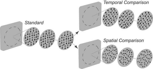
Random dot kinematograms (RDKs; examples shown in Fig. 1) were generated on a PC computer running custom software written in Python, using components of Psychopy (Peirce, 2007). Stimuli were displayed on an IIyama Vision Master Pro 514 CRT with a resolution of 1280 × 1024 pixels, update rate of 75 Hz at a viewing distance of 76.3 cm. Each RDK was generated anew prior to its presentation on each trial. Each image in a motion sequence consisted of 226 dots (luminance 0.05 cd/m²) displayed within a circular window (6 deg radius) on a uniform luminance background (25 cd/m²). Continuous apparent motion was produced by presenting the images consecutively at an update rate of 18.75 Hz, which is comparable to our previous work (Webb et al., 2007) and that used in other studies of global motion (e.g. Williams and Sekuler, 1984; Watamaniuk et al., 1989; Watamaniuk & Sekuler, 1992; Edwards and Badcock, 1995). Dot density and diameter were 2 dots/deg² and 0.1 deg, respectively. On the first frame in a motion sequence, dots were randomly positioned in the circular window and were displaced at 5 deg/sec. Dots that fell outside were wrapped to the opposite side of the window.

Figure 1.

Examples of random-dot-kinematograms (RDKs) used in the temporal and spatiotemporal experiments. In each experiment, observers judged whether sequentially presented standard or comparison RDKs had a more clockwise direction of motion. Temporal and spatial dot directions were sampled with replacement from an asymmetrical probability distribution with distinct measures of central tendency. All dots in the temporal comparison were displaced in the same randomly sampled direction on each image, generating a temporal sequence of directions across images; individual dots in the spatial comparison were displaced in independently sampled directions on each image, generating a spatial distribution of directions on each image. The comparison RDKs used for the spatiotemporal experiments consisted of different mixtures of spatial and temporal dot directions.

Psychophysical procedure

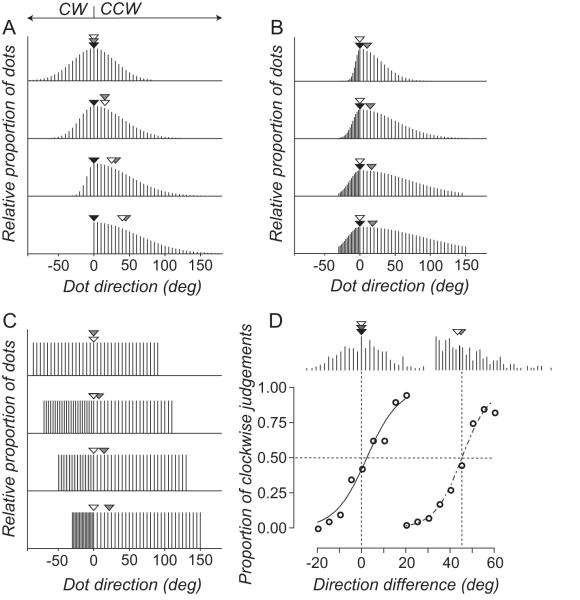
In a temporal two-alternative forced choice task, observers judged which of two RDKs had a more clockwise direction of motion. On each trial, standard and comparison RDKs (see Fig. 1) were presented in a random temporal order separated by a 1000 msec interval containing a fixation cross (luminance 0.05 cd/m²) on a uniform luminance background. The standard RDK was always composed of dots which moved in a common direction on each trial, randomly chosen from a uniform distribution spanning 360 deg. The comparison RDK was composed of dot directions drawn from a probability distribution with distinct measures of central tendency (see Fig. 2A-C).

Figure 2.

(A-C) Distributions of dot directions for different comparison RDKs. Arrows show the median (white), vector average (gray) and modal (black) direction of the comparison RDKs. (D) Directions sampled with replacement from the comparison distributions shown in the top and bottom panels of (A). When the comparison distribution is symmetrical the perceived direction of the standard RDKs aligns with the three measures of central tendency of the comparison RDK. When the comparison distribution is asymmetrical only the vector average direction aligns with the perceived direction of the standard RDK The smooth lines through the data points are the best fitting solutions to Equation 1.

Temporal pooling experiments: both comparison and standard RDKs consisted of 25 images, presented for a total duration of 1300 msec. The comparison dots were all displaced in a common direction on each image, sampled randomly and independently from the distribution, generating a temporal sequence of directions.

In the first two experiments, the temporal statistics of the comparison RDK were manipulated by independently varying the standard deviation (SD) of the half widths of the distribution, assigning the left half as the clockwise (CW) SD and the right half as the counter clockwise (CCW) SD. For the first experiment, dots directions were sampled at 5 deg intervals from a Gaussian distribution with a range of 180 deg. The SD of the CCW half of the Gaussian was either 30, 40, 50 or 60 deg; corresponding values on the CW half were 30, 20, 10 or 0 deg, generating asymmetrically distributions of dot directions with an increasingly distinct mode (Fig. 2A). For the second experiment, dot directions of the comparison RDK were sampled from a Gaussian with CCW SDs of 30, 50, 70 or 90 deg and CW SDs of 6, 10, 14 or 18 deg. Each half of the distribution was sampled at 5 and 1 deg intervals, respectively, generating asymmetrical distributions of dot directions with an increasingly distinct vector average (Fig 2B). For both experiments, the modal direction of the comparison RDK was randomly chosen on each trial using the Method of Constant Stimuli. In the third experiment, dots directions for the comparison RDK were sampled from a uniform distribution with a total range of 180°. We assigned each half of the distribution a different range and sampling density, sampling the CCW half at 5 deg intervals over a range of 90, 110, 130 or 150 deg and CW half in linear intervals over a range of 90, 70, 50 or 30°. This generated asymmetrical distributions with increasingly different medians and vector averages (Fig 2C). The median direction of the comparison RDK was randomly chosen on each trial using the Method of Constant Stimuli.

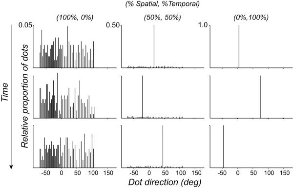
Spatiotemporal pooling experiments: both the comparison and standard RDKs consisted of 2, 4 or 8 images, presented consecutively for a total duration of 104, 208 or 416 msec. The comparison RDK consisted of different mixtures of “spatio-temporal” (100-0%) and “temporal” (0-100%) dot directions. “Spatio-temporal” dot directions are hereafter referred to as “spatial”. “Spatial” directions were sampled independently from each other on the current image and from their own direction on previous images; “temporal” dots were displaced in a common direction on each image, independently of their direction on previous images. “Spatial” and “temporal” dot directions were sampled in different proportions, with replacement, from a single asymmetrical uniform distribution (see Figure 5). We chose this distribution because it is diagnostic at distinguishing the predictions of a vector average from a maximum likelihood read-out of perceived direction (Webb et al., 2007). The median direction of the comparison RDK was randomly chosen on each trial using the Method of Constant Stimuli.

Figure 5.

Spatial and temporal dot directions sampled in different proportions from a single asymmetrical uniform distribution. Rows show different relative percentages of spatial and temporal dot directions. Columns show the samples obtained over time on each positional update of the dots.

Data analysis

For each experiment, observers completed a minimum of two runs of 180 trials. Data were expressed as the proportion of trials on which subjects judged the comparison RDK to be more CW than the standard RDK as a function of the angular difference between them. Each psychometric function was fitted with a logistic of the form:

$$P_{cw}=1∕(1+\exp ((\mu -\mathrm{x})∕\beta \left)\right),$$ 1

where P_cw is the proportion of clockwise judgements, μ is the stimulus level at which observers perceived the directions of the standard and comparison to be the same (point of subjective equality or PSE), and β is an estimate of direction discrimination threshold. Figure 2D shows psychometric functions obtained in the temporal pooling experiment.

Population decoding

Basic model

We begin with a brief description and then detail the full mathematical implementation of the model simulations. We simulated observers’ trial-by-trial performance on the temporal and spatiotemporal tasks with a physiologically-inspired population decoding model (c.f. Webb et al., 2007). The stimuli, timing, psychophysical procedure and number of trials were the same in the model simulations and human experiments. On each trial, we accumulated the spiking responses of a population of model direction-selective neurons to the comparison and standard RDKs. The central tendency direction of the comparison was randomly chosen on each trial using the Method of Constant Stimuli. A decoder “read-out” the population responses to the standard and comparison and judged which RDK had a more clockwise direction of motion. Psychometric functions based on the model response were accumulated for different forms of decoder.

Wherever practical our model and manipulations of its parameters were designed to mimic the behavior of an MT population. The model consists of 360 independently responsive, direction-selective neurons, where adjacent neurons’ preferred directions are separated by 1 deg. The sensitivity of the ith neuron, centered at θ_i to direction θ is:

$$S_i\left(\theta \right)=\exp \left\{-{\left[\right(\theta -{\theta }_i∕h]}^2\log 2\right\}$$ 2

where h is the bandwidth (half-height, half-width), fixed at 45 deg. This bandwidth is chosen to be within the range obtained in previous psychophysical studies on the directional tuning of motion mechanisms (Levinson and Sekuler, 1980; Raymond, 1993; Fine et al., 2004) and physiological studies on the directional tuning of MT neurons (Albright, 1984; Felleman and Kaas, 1984; Britten and Newsome, 1998). The response of the ith neuron to a distribution of dots directions D(θ) is:

$$R_i\left(D\right)=k\sum _{\theta =1}^{360}{S}_i\left(\theta \right)\mathrm{pr}\left\{D\right(\theta \left)\right\}\text{where}k=R_{\mathit{max}}t.$$ 3

R_max is the maximum firing rate of the neuron (60 spikes/s), is stimulus duration and pr{D(θ)} is the proportion of dot directions. The spiking response ( n_i ) is Poisson distributed with a mean of R_i(D)

$$p\left(n_{i}D\right)=\frac{R_i\left(D\right){{}^n}_i}{n_i!}\exp \{-R_i(D\left)\right\}$$ 4

We considered three different physiologically-plausible population decoders’ estimates of D. The log likelihood of D was computed by multiplying the response of each neuron by the log of its tuning function (Seung and Sompolinsky, 1993; Jazayeri and Movshon, 2006):

$$\log L\left(D\right)=\sum _{i=1}^{360}{n}_i\log R_i\left(D\right).$$ 5

The maximum likelihood direction estimated from the population response is the value of θ_i for which logL(D) for all D is maximal.

To estimate D with a winner-takes-all decoder, we read-off the value of θ_i where n_{i max} .

To obtain the corresponding estimate from a vector average decoder we calculated the average of the preferred directions of all neurons weighted in proportion to their response magnitude:

$$V_{\mathit{est}}^{\to }={\tan }^{-1}\left(\frac{\sum _{i=1}^{360}{n}_i\sin \left({\theta }_i\right)}{\sum _{i=1}^{360}{n}_i\cos \left({\theta }_i\right)}\right)$$ 6

Model parameter manipulations

To test systematically whether a likelihood-based pooling computation alone could accommodate observers’ psychophysical performance in the spatiotemporal pooling experiment, we parametrically manipulated the behavior of our direction tuned model neurons.

First, we varied number of neurons in the population in the range N = 12-720. Second, we varied the level at which the ith neuron’s response could reach saturation, such that:

$$R_D=\sum _{i=1}^{360}{R}_{\mathit{sat}}\frac{\theta }{{}^i(\theta +{\theta }_{50}^{\eta })}$$ 7

where R_sati is a fixed level of response saturation, is direction and θ₅₀is the number of dot directions at which the response reaches half its saturating level (fixed at 20), and η is the slope of the curve (fixed at 0.5).

Third, we conferred temporal dynamics on the ith neuron’s response with a decaying exponential of the form:

$$R_{t,D}=\sum _{i=1}^{360}{R}_{{\mathit{sus}}_i}+(R_{\max }-R_{{\mathit{sus}}_i}){\exp }^{-t∕{\tau }_r}$$ 8

where R_susi is the sustained part of the response, R _{max i} is the maximum response,τ_r is a time constant and t is time (Priebe et al., 2002).

Fourth, we implemented a simple form of temporal summation in which the ith neuron accumulates local motion signals on its receptive field as a power function of time, such that:

$$\sum (t,D)\sum _{i=1}^{360}\omega t^{{\tau }_D}$$ 9

where ω is a scaling factor, τ_D is a time constant and t is time.

Fifth, within each simulated trial we imposed a correlation structure on the noise in our population of neurons. Using a method described by Huang and Lisberger (2009), we first compute the desired correlation structure (c) across the ith and jth pairs of neurons as

$$c_{i,j}=C_{\max }\exp \left[\frac{-{\left(\Delta P{D}_{i,j}\right)}^2}{{\left(\Delta P{D}_{\max }{\mathrm{T}}_d\right)}^2}\right],$$ 10

where c_max is the maximum possible correlation between all pairs of neurons, ΔPD_{i, j} is the difference in preferred directions of pairs of neurons, T_d is rate at which correlations decay as a function of ΔPD, and ΔPD_max is fixed at 180 deg. Using a method developed by Shadlen et al. (1996) we enforce the desired noise correlations across the population by calculating the matrix square root (Q ) of the desired correlation matrix

$$c=Q{Q}^{\prime }$$ 11

such that every eigenvalue has a non-negative real part. We then multiply a vector of independent normal deviates with unit variance and zero mean (z) by Q

$$y=Qz,$$ 12

generating a matrix with covariance c. To derive a matrix of responses with a given correlation structure, we scale and offset y. The responses of the population to a distribution of dot directions can then be calculated as:

$$R_{ic}\left(D\right)=R_i\left(D\right)+\sqrt{R_i\left(D\right)y_i},$$ 13

where R_ic(D) is a 1 by N vector of correlated responses that depend on each neuron’s direction preference (θ_i) (For a complete derivation and discussion of this approach, see Shadlen et al. (1996), APPENDIX 1: Covariance).

Results

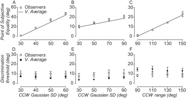
We first ask which pooling computations govern performance on a task that required human observers to combine local motion directions over time (temporal pooling experiment). Each psychometric function was fitted with a logistic (Equation 1; see Fig. 2D) to determine the stimulus level at which observers perceived the global directions of the standard and comparison RDKs to be the same (point of subjective equality or PSE). Figure 2D shows that skewing the distribution of directions in the comparison RDK caused a large (~45 deg) shift in the perceived direction of this observer away from the modal towards the median and vector average direction. This huge shift in perceived direction occurred without a concomitant change in the precision of discrimination performance (slopes of the two psychometric functions are similar).

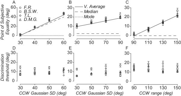
The behavior of this individual was representative of the performance of all observers. Perceived direction corresponded very closely to the vector average stimulus direction calculated over time, diverging substantially from the modal and median direction of motion. Figure 3A-C shows how the perceived direction of all observers changes as a function of skew in different comparison distributions (Fig. 2A-C). Symbols represent each subject’s PSE; dotted, dashed and solid lines represent the modal, median and vector average direction of motion of the comparison RDK, respectively. When the comparison RDK was generated from a Gaussian distribution with a CCW SD of 60 deg (Fig. 2A bottom panel), the modal direction of the comparison had to be rotated by ~45 deg, on average, for the standard and comparison to be perceived moving in the same direction (Fig. 3A). With a CCW SD of the dot distribution equal to 90 deg, the modal direction of the comparison needed to be rotated by about 20 degrees in order for observers to perceive the comparison and the standard moving in the same direction (Fig. 3B). Similarly, when comparison directions were drawn from a uniform distribution with CCW range of 150 deg, the median direction had to be rotated by about 20 degrees to be perceived moving in the same direction as the standard (Fig. 3C). Unlike perceived direction, observers’ discrimination thresholds were relatively independent of degree of skew in the comparison distributions (Fig. 3D-F).

Figure 3.

Vector average of direction distributions accumulated over time predicts the temporal pooling of local motion directions. (A-C) Symbols show the perceived direction of four observers as a function of different comparison distributions. Lines show the temporal vector average (solid), median (dashed) and modal (dotted) direction of the comparison distribution. (B) Note the median direction has been offset from the mode to reduce clutter. (D-F) Symbols show the direction discrimination thresholds of four observers as a function of different comparison distributions. Error bars are 95% CI.

A vector average read-out (Equation 6) from a model population of direction-selective neurons (see Materials and Methods for basic model details) also predicted observers’ perceived direction (Fig. 4A-C) and the pattern of discrimination thresholds (Fig. 4D-F) in the temporal pooling experiment. This finding contrasts with our previous work, where we found that maximum likelihood was a robust estimator of performance on a task that required observers to pool local motion samples across space (Webb et al., 2007). These discrepant results appear consistent with the notion of a flexible motion pooling system which can adopt different computations to address different stimulus demands, as others have found for the perception of rigid motion (Stone et al., 1990; Yo and Wilson, 1992; Burke and Wenderoth, 1993; Lorenceau et al., 1993; Cropper et al., 1994; Bowns, 1996; Amano et al., 2009).

Figure 4.

Vector average read-out from a physiologically imspired model predicts the temporal pooling of local motion directions. (A-C) White circles show the average perceived direction of four observers as a function of different comparison distributions. Solid lines show the perceived directions estimated by a vector average decoder (Equation 6). (D-F) White circles show the average direction discrimination thresholds of four observers as a function of different comparison distributions. Black circles show vector average decoder’s estimate of direction discrimination thresholds. Error bars are 95% CI.

To test whether a flexible pooling process can account of these discrepant results, we designed an additional experiment containing components of the previous two. The task and design were the same as above with the following exceptions. The comparison RDK consisted of different mixtures of “spatial” and “temporal” dot directions and was presented at three different stimulus durations (See Materials and Methods). All dot directions in the comparison RDK were drawn, with replacement, from a distribution which was particularly diagnostic at distinguishing between the predictions of a maximum likelihood and vector average read-out of perceived motion direction. Figure 5 shows examples of how we sampled different mixtures of “spatial” and “temporal” directions from this distribution. Note how the temporal dot directions dominate when the numbers of spatial and temporal dots are equally balanced in the comparison distribution (50% spatial, 50% temporal). The predominance of temporal directions in spatiotemporal motion stimuli tightly constrains the behavior of model neurons which can accommodate performance on the spatiotemporal pooling task. We will return to this important point below.

Figure 6 and 7 shows the performance of observers in the spatiotemporal experiment. Perceived direction (Fig. 6) and discrimination thresholds (Fig. 7) are plotted for three different stimulus durations as a function of the percentage of temporal dots in the comparison (Note that the percentage of temporal dots is inversely related to the percentage of spatial dots). Varying the mixture of temporal and spatial dots in the comparison RDK caused large (up to 25 deg) shifts in observer’s perceived direction, PSEs varying between −10 (100% spatial dots) and 15 deg (100% temporal dots). Stimulus duration modulated this relationship between perceived direction and percentage of temporal dots in the comparison - an effect that was most apparent when the numbers of spatial and temporal dots were equally balanced (Fig. 6). For all observers, increasing the relative percentage of temporal dots (thus reducding percentage of spatial dots) in the comparison RDK caused discrimination thresholds to rise. For one observer (F.R.) the relationship between discrimination thresholds and percentage of temporal dots was modulated by stimulus duration: thresholds were larger at shorter stimulus durations. This effect was not marked for the other two observers.

Figure 6.

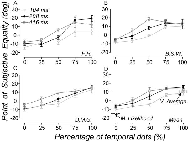
Different population decoders predict the spatial and temporal pooling of local motion directions. (A-C) Symbols show the perceived direction of three observers at three stimulus durations, plotted as a function of the percentage of temporal dots (inversely related to the percentage of spatial dots) in the comparison. (D) Symbols show the average perceived direction of observers plotted and notated as in (A-C). Dashed lines on the right are the perceived direction at three stimulus durations estimated by a vector average decoder (Equation 6) when all the dots are “temporal”; black dashed lines on the left of the plot are the perceived direction at three stimulus durations estimated by a maximum likelihood decoder (Equation 5) when all of dots are “spatial” (the maximum likelihood estimates are the same for the three durations). Error bars are 95% CI.

Figure 7.

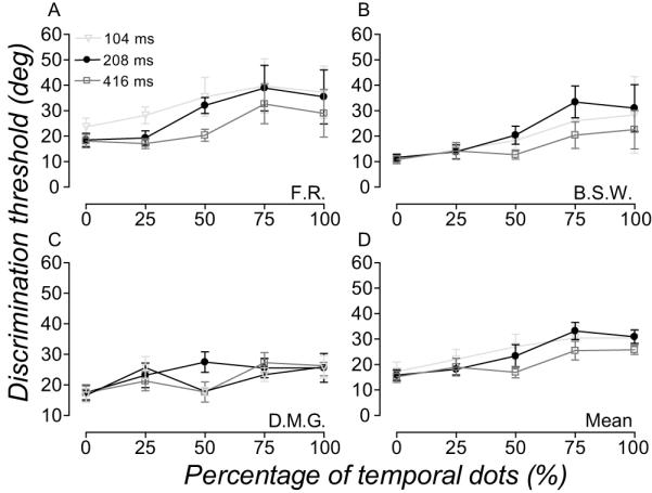
Direction discrimination thresholds in the spatiotemporal pooling experiment. (A-C) Symbols show the direction discrimination thresholds of three observers at three stimulus durations, plotted as a function of the percentage of temporal dots in the comparison. (D) Symbols show the average direction discrimination thresholds of observers plotted and notated as in (A-C). Error bars are 95% CI.

Figure 6D shows the average perceived direction of the three observers. The dashed lines on the right show that a vector average decoder (Equation 6) accurately estimated perceived direction at the three stimulus durations (indicated by different shades of grey) when RDKs were populated by temporal dots. In contrast, a maximum likelihood decoder (Equation 5) accurately estimated perceived direction at the three stimulus durations (indicated by a single black dashed line because the estimates were the same for three durations) when RDKs were populated by spatial dots. Yet with either population decoder alone, we were unable predict the duration-dependence of the relationship between perceived direction and percentage of temporal dots in the comparison. These data suggest a flexible form of motion pooling, one that uses different computations in space and time.

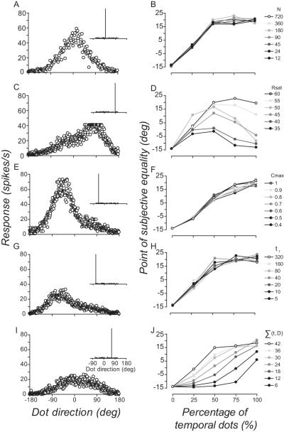
In principle, a single, likelihood-based computation could account for the dynamics of spatiotemporal motion pooling. Likelihoods are derived from the tuning and response properties of individual motion sensitive neurons (Jazayeri and Movshon, 2006), which raises the possibility that the behavior of the input neurons rather than the pooling computations themselves govern the flexibly of spatiotemporal motion pooling. Our basic model neurons lacked many of the well known characteristics of motion-sensitive neurons, including non-linear response saturation (e.g. Albrecht & Geisler, 1991, Sclar, Maunsell & Lennie, 1990), temporal response integration (for reviews see Born, Tsui & Pack, 2009, Smith, Majaj & Movshon, 2009), temporal summation (e.g. Snowden and Braddick, 1991; Watamaniuk and Sekuler, 1992; Burr and Santoro, 2001) and a correlation structure to the noise across the population of neurons (e.g. Bair, Zohary & Newsome, 2001, Kohn & Smith, 2005, Zohary, Shadlen & Newsome, 1994). To test whether a likelihood-based pooling computation alone could accommodate observers’ psychophysical performance in the spatiotemporal pooling experiment, we systematically introduced some of these characteristics to our population of MT neurons (for details, see Materials and Methods). The left column in Figure 8 shows examples of the effects of manipulating the model neurons’ behavior on the response of the population when the numbers of spatial and temporal directions are equally balanced in the comparison distribution (50% spatial, 50% temporal). Samples from the distribution (inset in each panel) were presented to the model for a total duration of 104 ms (2 images). The right column shows how these manipulations of the model neurons changes a maximum likelihood read-out (Equation 5) of the relationship between perceived direction and percentage of temporal dots in the comparison.

Figure 8.

Effects of manipulating the behavior of input neurons on maximum likelihood’s estimate of perceived direction in the spatiotemporal pooling experiment. Left column shows basic model population responses to of equally balanced (50%, 50%) spatial and temporal samples from a comparison distribution (inset in each panel), presented for a total duration of 104 ms. The left panels show examples of changes to the shape of the population response caused by varying: (A) numbers of neurons in the population (N = 180 neurons); (B) level at which neurons’ responses saturate (Equation 7, R_sat = 40 spikes/s); (C) correlation structure of the interal noise across the population of neurons (Equation 10, C _max = 0.5); (D) time constant of temporal response integration (Equation 8, τ_r = 20 ms); and (E) rate at which neurons respond to the number of dot directions on their receptive fields (Equation 9, ∑(t, D) =18). Right column shows how varying the model parameters N, R_sat , C _max , τ_r and ∑(t, D) modulated maximum likelihood’s estimate of perceived direction in the spatiotemporal experiment. Varying the rate at which neurons respond to the total number of dots on their receptive field was the only manipulation to the basic model which approximated observers’ performance at different stimulus durations.

When the numbers of spatial and temporal dots were equally balanced in the comparison they did not have equivalent effects on the population response (N = 180 neurons). As the temporal dots all had the same direction this inevitably swamped the population response, negating the relative contribution of spatial directions (Fig. 8A). The predominance of temporal directions saturated maximum likehood’s estimate of perceived direction. Varying the the total number of neurons in the population (N=12-720) had very little impact on this effect: maximum likelihood produced equivalent estimates of perceived direction regardles of whether the comparison stimulus was populated by 50, 75 or 100% of temporal directions (Fig. 8B).

We attempted to mitigate the effects on the read-out by fixing the the level at which all neurons’ responses saturate. This flattened the peak of the population response (Fig. 8C; Equation 7, R_sat = 40 spikes/s) and eradicated the saturation of maximum liklihood’s estimate of perceived direction, particularly when temporal directions outweighed spatial directions (Fig. 8D). However, we could not find a fixed level of response saturation that produced maximum likelihood estimates of perceived direction which corresponded to observers’ pattern of performance in the spatiotemporal experiment (Fig. 6).

Perfectly correlated noise between neurons with similar direction preferences (Equation 10, C _max = 1) with correlation strength decaying as a function of the difference in preferred directions of pairs of neurons (Equation 10, T_d = 0.5) both increased and broadened the peak of the population response (Fig 8E). Different patterns of correlated noise across the population mitigated the saturating effects on the read-out such that the gradient of the relationship between the maximum likelihood perceived direction and percentage of temporal dots (Fig. 8F) was very similar to that of observers (Fig. 6). However, changes to the noise structure did not accomodate the way in which stimulus duration modulated this relationship.

Conferring a form of temporal integration where each neuron’s response has a maximum (Equation 8, R _max i = 60 spikes/s) and decays to a sustained level (Equation 8, R_susi = 2 spikes/s) exponentially over time (Equation 8, τ = 20 ms) both reduced and slightly broadened the population response (Fig. 8G). But varying the time constant of integration (τ) did not capture the way in which stimulus duration affects performance on this task (Fig. 8H).

Our last manipulation to the model is built on a well known characteristic of motion sensitive neurons in MT: responses saturate at very small numbers of dot directions (Snowden et al., 1991; Snowden et al., 1992). Implementing a simple form of temporal summation where each neuron accumulates local directional signals present within its receptive field as a power function of time (Equation 9, ∑(t, D) ) both reduced and broadened the population response (Fig. 8I). Together these changes to the population response were suffcient to counteract the dominance of temporal directions and boost the relative contribution of spatial directions to the read-out. By fixing the rate at which neuron’s accumulated direction signals, maximum likilihood was able to read-out different numbers of directions over different time epochs. This simple, physiologically plausible change to the direction-selective neurons produced a family of functions (Fig. 8J) that closely approximates the relationship we found in the spatiotemporal experiment.

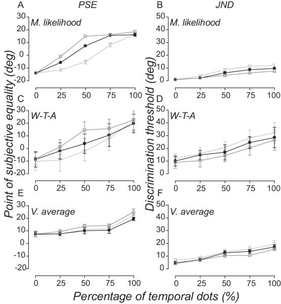
Figure 9A show the maximum likelihood read-out from this model which most accurately predicts observers’ perceived direction in the spatiotemporal experiment. When the input neurons summed local directions at a fixed temporal rate (Equation 9, τ_D = 0.36), the correspondence between the model predictions and observers performance (Fig. 6D) is striking. [This model can also accommodate observers’ performance in the temporal experiments (data not shown)]. For comparison, we decoded corresponding estimates of perceived direction from same population of neurons using winner-takes-all (Fig. 9C) and vector average (Fig. 9E). Winner-takes-all predictions are relatively accurate but hugely variable, and vector average predictions diverged substantially from the empirical data. All three decoders produced predictions which captured the relative change in observers’ discrimination thresholds as the percentage of temporal directions increase (and percentage of spatial directions decrease) in the spatiotemporal experiment (Fig 9B, D & F). Yet only winner-takes-all approximated the absolute threshold levels (Fig 9D.).

Figure 9.

Computations governing spatiotemporal pooling of local motion directions. (A) Maximum likelihood read-out from model neurons which sum local directions at a fixed rate over time (Equation 9, τ_D = 0.36) accurately predicts human observers’ perceived direction at different stimulus durations in the spatiotemporal pooling experiment. Corresponding estimates of perceived direction from winner-takes-all and vector average decoders are accurate but hugely variable (C) and completely inaccurate (E), respectively. Maximum likelihood (B), winner-takes-all (D) and vector average (F) decoders all approximate the general pattern of observers’ direction discrimination thresholds in the spatiotemporal pooling experiment. Error bars are 95% CI.

Discussion

A simple computational model built on realistic physiological principles could accommodate the dynamic nature of human observers’ psychophysical performance on two tasks which required the pooling of motion directions over space and time. We did not have to invoke an adaptive pooling mechanism that derives different computational solutions over space and time to explain observers’ perception. Our modeling suggested a more parsimonious solution, whereby the flexible nature of spatiotemporal pooling can be accommodated by a single computation that optimally pools motion signals across a population of neurons which effectively “count” the total number of dots on their receptive fields at a fixed rate over time.

Our results suggest that flexible pooling emerges naturally from the dynamics of the input neurons rather than residing with the pooling computations themselves. This conclusion differs from other psychophysical studies of motion perception (Stone et al., 1990; Stone and Thompson, 1992; Yo and Wilson, 1992; Burke and Wenderoth, 1993; Lorenceau et al., 1993; Cropper et al., 1994; Bowns, 1996; Zohary et al., 1996; Amano et al., 2009), which suggest that the visual system can adaptively switch between different pooling computations depending upon the nature of the stimulus. Many studies have found that different pooling computations coincide with the perception of weak (low contrast, short duration, 1-D), and strong (high contrast, long duration, 2-D) forms of rigid motion. Moreover, when a distribution of dot directions is skewed asymmetrically, the perceived direction can be biased away from the mean towards the modal direction of global motion (Zohary et al., 1996), suggesting that the visual system has access to the entire distribution of local directions and adopts a flexible decision strategy (Zohary et al., 1996). Yet it is not clear how the brain decides on which computations to choose within an adaptive pooling framework. Much of the psychophysical evidence in favor of adaptive pooling does not distinguish stimulus-from mechanism-based pooling computations (Stone et al., 1990; Stone and Thompson, 1992; Yo and Wilson, 1992; Burke and Wenderoth, 1993; Lorenceau et al., 1993; Cropper et al., 1994; Bowns, 1996; Zohary et al., 1996; Amano et al., 2009). Without distinguishing the computational description of a visual stimulus from the underlying putative mechanism, it is impossible to know whether a single, mechanism-based computation can fully explain the pooling process. Indeed many of the adaptive rigid motion effects and the perceptual switch between different motion-based summary statistics can be accommodated by computational models that optimally read-out the motion percept with a single, likelihood computation (Weiss et al., 2002; Webb et al., 2007).

We have extended this work to show that computations built on well known physiological properties of MT neurons can accommodate flexible spatiotemporal pooling of local motion signals at a range of stimulus durations in human vision. Temporal pooling improves the precision with which motion signals can be discriminated (van Doorn and Koenderink, 1982; Snowden and Braddick, 1991; Watamaniuk and Sekuler, 1992; Fredericksen et al., 1994; Neri et al., 1998; Burr and Santoro, 2001), but the time window over which signals are accumulated depends upon speed, spatial frequency, contrast and temporal structure of the stimulus (Nachmias, 1967; Vassilev and Mitov, 1976; van Doorn and Koenderink, 1982; Thompson, 1982 ; De Bruyn and Orban, 1988; Bialek et al., 1991; Buracas et al., 1998; Bair and Movshon, 2004). Even though responses saturate at very small numbers of dot directions (Snowden et al., 1991; Snowden et al., 1992) and most of the information about the direction of constant motion is available soon after stimulus onset, MT neurons can transmit more information about stimuli with rich temporal structure (Buracas et al, 1998). Our modeling predicts that the way in which motion sensitive neurons respond to stimuli with rich temporal structure also contributes to the flexible pooling of motion signals read-out from MT. The form of temporal summation is not critical to this argument. In our model, the rate at which MT neurons accumulate local directions grew exponentially over time, but the type of temporal summation described in other psychophysical studies (Snowden and Braddick, 1991; Watamaniuk and Sekuler, 1992; Fredericksen et al., 1994; Neri et al., 1998; Burr and Santoro, 2001) may well have performed equally well.

A few studies have emphasized the contribution of rapidly saturating MT responses at small numbers of dot directions (Snowden et al., 1991; Snowden et al., 1992) to the pooling of local motion signals (Simoncelli and Heeger, 1998; Dakin et al., 2005), but to our knowledge none have shown how the temporal accumulation of local motion signals mediates flexible pooling. Counting the number of dot directions is equivalent to summing motion energy (Britten et al., 1993), and our results are broadly consistent with the notion that motion-sensitive neurons behave like spatiotemporal energy detectors (Watson and Ahumada, 1983; van Santen and Sperling, 1984; Adelson and Bergen, 1985; Watson and Ahumada, 1985; Heeger, 1987; Simoncelli and Heeger, 1998). Recent models of visual motion pooling have extended motion energy models and shown how the non-linear dynamics of input neurons can contribute to the subsequent pooling of visual motion signals (Rust et al., 2006; Tsui1 et al., 2010), reinforcing the notion that the complex dynamics of spatiotemporal pooling is inherited rather than adaptively computed at the pooling stage.

Conclusion

We have shown that a single, likelihood-based computation can accommodate the flexible nature of spatiotemporal motion pooling in human vision. Because likelihoods are derived from the tuning and response properties of individual motion sensitive neurons, flexible pooling emerges naturally from the temporal dynamics of these input neurons. This general principle obviates the need to invoke different computations to accommodate the complex dynamics of motion pooling.

References

- Adelson EH, Bergen JR. Spatiotemporal energy models for the perception of motion. J Opt Soc Am A. 1985;2:284–299. doi: 10.1364/josaa.2.000284. [DOI] [PubMed] [Google Scholar]
- Alais D, Burr D. The ventriloquist effect results from near-optimal bimodal integration. Curr Biol. 2004;14:257–262. doi: 10.1016/j.cub.2004.01.029. [DOI] [PubMed] [Google Scholar]
- Albrecht DG, Geisler WS. Motion selectivity and the contrast-response function of simple cells in the visual cortex. Visual Neuroscience. 1991;7:531–546. doi: 10.1017/s0952523800010336. [DOI] [PubMed] [Google Scholar]
- Albright TD. Direction and orientation selectivity of neurons in visual area MT of the macaque. J Neurophysiol. 1984;52:1106–1130. doi: 10.1152/jn.1984.52.6.1106. [DOI] [PubMed] [Google Scholar]
- Amano K, Edwards M, Badcock DR, Nishida S. Adaptive pooling of visual motion signals by the human visual system revealed with a novel multi-element stimulus. Journal of Vision. 2009;9:1–25. doi: 10.1167/9.3.4. [DOI] [PubMed] [Google Scholar]
- Bair W, Movshon JA. Adaptive temporal integration of motion in direction-selective neurons in macaque visual cortex. J Neurosci. 2004;24:7305–7323. doi: 10.1523/JNEUROSCI.0554-04.2004. [DOI] [PMC free article] [PubMed] [Google Scholar]
- Bair W, Zohary E, Newsome WT. Correlated firing in macaque visual area MT: time scales and relationship to behavior. J Neurosci. 2001;21:1676–1697. doi: 10.1523/JNEUROSCI.21-05-01676.2001. [DOI] [PMC free article] [PubMed] [Google Scholar]
- Barthelemy FV, Fleuriet J, Masson GS. Temporal dynamics of 2D motion integration for ocular following in macaque monkeys. J Neurophysiol. 2010;103:1275–1282. doi: 10.1152/jn.01061.2009. [DOI] [PubMed] [Google Scholar]
- Bialek W, Rieke F, de Ruyter van Steveninck RR, Warland D. Reading a neural code. Science. 1991;252:1854–1857. doi: 10.1126/science.2063199. [DOI] [PubMed] [Google Scholar]
- Born RT, Bradley DC. Structure and function of visual area MT. Annu Rev Neurosci. 2005;28:157–189. doi: 10.1146/annurev.neuro.26.041002.131052. [DOI] [PubMed] [Google Scholar]
- Born RT, Tsui JMG, Pack CC. Temporal dynamics of motion integration. In: Ilg UW, Masson GS, editors. Dynamics of Visual Motion Processing. Springer Verlag; NewYork: 2009. pp. 37–54. [Google Scholar]
- Born RT, Pack CC, Ponce CR, Yi S. Temporal evolution of 2-dimensional direction signals used to guide eye movements. J Neurophysiol. 2006;95:284–300. doi: 10.1152/jn.01329.2004. [DOI] [PubMed] [Google Scholar]
- Bowns L. Evidence for a feature tracking explanation of why type II plaids move in the vector sum direction at short durations. Vision Res. 1996;36:3685–3694. doi: 10.1016/0042-6989(96)00082-x. [DOI] [PubMed] [Google Scholar]
- Braddick O. Segmentation versus integration in visual motion processing. Trends Neurosci. 1993;16:263–268. doi: 10.1016/0166-2236(93)90179-p. [DOI] [PubMed] [Google Scholar]
- Britten K, Newsome W. Tuning bandwidths for near-threshold stimuli in area MT. J Neurophysiol. 1998;80:762–770. doi: 10.1152/jn.1998.80.2.762. [DOI] [PubMed] [Google Scholar]
- Britten KH, Shadlen MN, Newsome WT, Movshon JA. Responses of neurons in macaque MT to stochastic motion signals. Vis Neurosci. 1993;10:1157–1169. doi: 10.1017/s0952523800010269. [DOI] [PubMed] [Google Scholar]
- Buracas GT, Zador AM, DeWeese MR, Albright TD. Efficient discrimination of temporal patterns by motion-sensitive neurons in primate visual cortex. Neuron. 1998;20:959–969. doi: 10.1016/s0896-6273(00)80477-8. [DOI] [PubMed] [Google Scholar]
- Burke D, Wenderoth P. The effect of interactions between one-dimensional component gratings on two-dimensional motion perception. Vision Res. 1993;33:343–350. doi: 10.1016/0042-6989(93)90090-j. [DOI] [PubMed] [Google Scholar]
- Burr DC, Santoro L. Temporal integration of optic flow, measured by contrast and coherence thresholds. Vision Res. 2001;41:1891–1899. doi: 10.1016/s0042-6989(01)00072-4. [DOI] [PubMed] [Google Scholar]
- Cropper SJ, Badcock DR, Hayes A. On the role of second-order signals in the perceived direction of motion of type II plaid patterns. Vision Res. 1994;34:2609–2612. doi: 10.1016/0042-6989(94)90246-1. [DOI] [PubMed] [Google Scholar]
- Dakin SC, Mareschal I, Bex PJ. Local and global limitations on direction integration assessed using equivalent noise analysis. Vision Res. 2005;45:3027–3049. doi: 10.1016/j.visres.2005.07.037. [DOI] [PubMed] [Google Scholar]
- De Bruyn B, Orban GA. Human velocity and direction discrimination measured with random dot patterns. Vision Res. 1988;28:1323–1335. doi: 10.1016/0042-6989(88)90064-8. [DOI] [PubMed] [Google Scholar]
- Dean AF. The variability of discharge of simple cells in the cat striate cortex. Exp Brain Res. 1981;44:437–440. doi: 10.1007/BF00238837. [DOI] [PubMed] [Google Scholar]
- Deneve S, Latham PE, Pouget A. Reading population codes: a neural implementation of ideal observers. Nat Neurosci. 1999;2:740–745. doi: 10.1038/11205. [DOI] [PubMed] [Google Scholar]
- Edwards M, Badcock DR. Global motion perception: no interaction between the first- and second-order motion pathways. Vision Res. 1995;35:2589–2602. doi: 10.1016/0042-6989(95)00003-i. [DOI] [PubMed] [Google Scholar]
- Ernst MO, Banks MS. Humans integrate visual and haptic information in a statistically optimal fashion. Nature. 2002;415:429–433. doi: 10.1038/415429a. [DOI] [PubMed] [Google Scholar]
- Felleman DJ, Kaas JH. Receptive-field properties of neurons in middle temporal visual area (MT) of owl monkeys. J Neurophysiol. 1984;52:488–513. doi: 10.1152/jn.1984.52.3.488. [DOI] [PubMed] [Google Scholar]
- Ferrera VP. Task-dependent modulation of the sensorimotor transformation for smooth pursuit eye movements. J Neurophysiol. 2000;84:2725–2738. doi: 10.1152/jn.2000.84.6.2725. [DOI] [PubMed] [Google Scholar]
- Fine I, Anderson CM, Boynton GM, Dobkins KR. The invariance of directional tuning with contrast and coherence. Vision Res. 2004;44:903–913. doi: 10.1016/j.visres.2003.11.022. [DOI] [PubMed] [Google Scholar]
- Foldiak P. The ‘ideal homunculus’: Statistical inference from neural population responses. In: Eeckman F, Bower J, editors. Computation and Neural Systems. Kluwer Academic Publishers; Norwell, MA: 1993. pp. 55–60. [Google Scholar]
- Fredericksen RE, Verstraten FA, Van de Grind WA. Temporal integration of random dot apparent motion information in human central vision. Vision Res. 1994;34:461–476. doi: 10.1016/0042-6989(94)90160-0. [DOI] [PubMed] [Google Scholar]
- Heeger DJ. Model for the extraction of frame flow. J Opt Soc Am A. 1987;4:1455–1471. doi: 10.1364/josaa.4.001455. [DOI] [PubMed] [Google Scholar]
- Huang X, Lisberger SG. Noise correlations in cortical area MT and their potential impact on trial-by-trial variation in the direction and speed of smooth-pursuit eye movements. J Neurophysiol. 2009;101:3012–3030. doi: 10.1152/jn.00010.2009. [DOI] [PMC free article] [PubMed] [Google Scholar]
- Hubel DH, Wiesel TN. Receptive fields, binocular interaction and functional architecture in cat’s visual cortex. J Physiol. 1962;160:106–154. doi: 10.1113/jphysiol.1962.sp006837. [DOI] [PMC free article] [PubMed] [Google Scholar]
- Jacobs RA. Optimal integration of texture and motion cues to depth. Vision Res. 1999;39:3621–3629. doi: 10.1016/s0042-6989(99)00088-7. [DOI] [PubMed] [Google Scholar]
- Jazayeri M, Movshon JA. Optimal representation of sensory information by neural populations. Nat Neurosci. 2006;9:690–696. doi: 10.1038/nn1691. [DOI] [PubMed] [Google Scholar]
- Kohn A, Smith MA. Stimulus dependence of neuronal correlation in primary visual cortex of the macaque. J Neurosci. 2005;25:3661–3673. doi: 10.1523/JNEUROSCI.5106-04.2005. [DOI] [PMC free article] [PubMed] [Google Scholar]
- Landy MS, Maloney LT, Johnston EB, Young M. Measurement and modeling of depth cue combination: in defense of weak fusion. Vision Res. 1995;35:389–412. doi: 10.1016/0042-6989(94)00176-m. [DOI] [PubMed] [Google Scholar]
- Levinson E, Sekuler R. A two-dimensional analysis of direction-specific adaptation. Vision Res. 1980;20:103–107. doi: 10.1016/0042-6989(80)90151-0. [DOI] [PubMed] [Google Scholar]
- Lorenceau J, Shiffrar M, Wells N, Castet E. Different motion sensitive units are involved in recovering the direction of moving lines. Vision Res. 1993;33:1207–1217. doi: 10.1016/0042-6989(93)90209-f. [DOI] [PubMed] [Google Scholar]
- Majaj NJ, Carandini M, Movshon JA. Motion integration by neurons in macaque MT is local, not global. J Neurosci. 2007;27:366–370. doi: 10.1523/JNEUROSCI.3183-06.2007. [DOI] [PMC free article] [PubMed] [Google Scholar]
- Masson GS. From 1D to 2D via 3D: dynamics of surface motion segmentation for ocular tracking in primates. J Physiol Paris. 2004;98:35–52. doi: 10.1016/j.jphysparis.2004.03.017. [DOI] [PubMed] [Google Scholar]
- Mingolla E. Neural models of motion integration and segmentation. Neural Netw. 2003;16:939–945. doi: 10.1016/S0893-6080(03)00099-6. [DOI] [PubMed] [Google Scholar]
- Nachmias J. Effect of exposure duration on visual contrast sensitivity with square-wave gratings. J Opt Soc Am [A] 1967;57:421–427. [Google Scholar]
- Neri P, Morrone MC, Burr DC. Seeing biological motion. Nature. 1998;395:894–896. doi: 10.1038/27661. [DOI] [PubMed] [Google Scholar]
- Pack CC, Born RT. Temporal dynamics of a neural solution to the aperture problem in visual area MT of macaque brain. Nature. 2001;409:1040–1042. doi: 10.1038/35059085. [DOI] [PubMed] [Google Scholar]
- Pack CC, Berezovskii VK, Born RT. Dynamic properties of neurons in cortical area MT in alert and anaesthetized macaque monkeys. Nature. 2001;414:905–908. doi: 10.1038/414905a. [DOI] [PubMed] [Google Scholar]
- Paradiso MA. A theory for the use of visual orientation information which exploits the columnar structure of striate cortex. Biol Cybern. 1988;58:35–49. doi: 10.1007/BF00363954. [DOI] [PubMed] [Google Scholar]
- Peirce JW. Psychopy - Psychophysics software in Python. J Neurosci Meth. 2007;162:8–13. doi: 10.1016/j.jneumeth.2006.11.017. [DOI] [PMC free article] [PubMed] [Google Scholar]
- Priebe NJ, Churchland MM, Lisberger SG. Constraints on the source of short-term motion adaptation in macaque area MT. I. the role of input and intrinsic mechanisms. J Neurophysiol. 2002;88:354–369. doi: 10.1152/.00852.2002. [DOI] [PMC free article] [PubMed] [Google Scholar]
- Raymond JE. Movement direction analysers: independence and bandwidth. Vision Res. 1993;33:767–775. doi: 10.1016/0042-6989(93)90196-4. [DOI] [PubMed] [Google Scholar]
- Recanzone GH, Wurtz RH. Shift in smooth pursuit initiation and MT and MST neuronal activity under different stimulus conditions. J Neurophysiol. 1999;82:1710–1727. doi: 10.1152/jn.1999.82.4.1710. [DOI] [PubMed] [Google Scholar]
- Regan D, Beverley KI. Postadaptation orientation discrimination. J Opt Soc Am A. 1985;2:147–155. doi: 10.1364/josaa.2.000147. [DOI] [PubMed] [Google Scholar]
- Rust NC, Mante V, Simoncelli EP, Movshon JA. How MT cells analyze the motion of visual patterns. Nat Neurosci. 2006;9:1421–1431. doi: 10.1038/nn1786. [DOI] [PubMed] [Google Scholar]
- Sanger TD. Probability density estimation for the interpretation of neural population codes. J Neurophysiol. 1996;76:2790–2793. doi: 10.1152/jn.1996.76.4.2790. [DOI] [PubMed] [Google Scholar]
- Schiller PH, Finlay BL, Volman SF. Short-term response variability of monkey striate neurons. Brain Res. 1976;105:347–349. doi: 10.1016/0006-8993(76)90432-7. [DOI] [PubMed] [Google Scholar]
- Sclar G, Maunsell JHR, Lennie P. Coding of frame contrast in central visual pathways of the macaque monkey. Vision Res. 1990;30:1–10. doi: 10.1016/0042-6989(90)90123-3. [DOI] [PubMed] [Google Scholar]
- Seung HS, Sompolinsky H. Simple models for reading neuronal population codes. Proc Natl Acad Sci U S A. 1993;90:10749–10753. doi: 10.1073/pnas.90.22.10749. [DOI] [PMC free article] [PubMed] [Google Scholar]
- Shadlen MN, Britten KH, Newsome WT, Movshon JA. A computational analysis of the relationship between neuronal and behavioral responses to visual motion. J Neurosci. 1996;16:1486–1510. doi: 10.1523/JNEUROSCI.16-04-01486.1996. [DOI] [PMC free article] [PubMed] [Google Scholar]
- Simoncelli EP, Heeger DJ. A model of neuronal responses in visual area MT. Vision Res. 1998;38:743–761. doi: 10.1016/s0042-6989(97)00183-1. [DOI] [PubMed] [Google Scholar]
- Smith MA, Majaj NJ, Movshon JA. Dynamics of motion signaling by neurons in macaque area MT. Nat Neurosci. 2005;8:220–228. doi: 10.1038/nn1382. [DOI] [PubMed] [Google Scholar]
- Smith MA, Majaj NJ, Movshon JA. Dynamics of Pattern Motion Computation. In: Ilg UW, Masson GS, editors. Dynamics of Visual Motion Processing. Springer Verlag; New York: 2009. pp. 55–72. [Google Scholar]
- Snowden RJ, Braddick OJ. The temporal integration and resolution of velocity signals. Vision Res. 1991;31:907–914. doi: 10.1016/0042-6989(91)90156-y. [DOI] [PubMed] [Google Scholar]
- Snowden RJ, Treue S, Andersen RA. The response of neurons in areas V1 and MT of the alert rhesus monkey to moving random dot patterns. Exp Brain Res. 1992;88:389–400. doi: 10.1007/BF02259114. [DOI] [PubMed] [Google Scholar]
- Snowden RJ, Treue S, Erickson RG, Andersen RA. The response of area MT and V1 neurons to transparent motion. J Neurosci. 1991;11:2768–2785. doi: 10.1523/JNEUROSCI.11-09-02768.1991. [DOI] [PMC free article] [PubMed] [Google Scholar]
- Stocker AA, Simoncelli EP. Noise characteristics and prior expectations in human visual speed perception. Nat Neurosci. 2006;9:578–585. doi: 10.1038/nn1669. [DOI] [PubMed] [Google Scholar]
- Stone LS, Thompson P. Human speed perception is contrast dependent. Vision Res. 1992;32:1535–1549. doi: 10.1016/0042-6989(92)90209-2. [DOI] [PubMed] [Google Scholar]
- Stone LS, Watson AB, Mulligan JB. Effect of contrast on the perceived direction of a moving plaid. Vision Res. 1990;30:1049–1067. doi: 10.1016/0042-6989(90)90114-z. [DOI] [PubMed] [Google Scholar]
- Thompson P. Perceived rate of movement depends on contrast. Vis Res. 1982;22:377–380. doi: 10.1016/0042-6989(82)90153-5. [DOI] [PubMed] [Google Scholar]
- Tsui1 JMG, Hunter JN, Born RT, Pack CC. The role of V1 surround suppression in MT motion integration. J Neurophys. 2010 doi: 10.1152/jn.00654.2009. [DOI] [PMC free article] [PubMed] [Google Scholar]
- van Doorn AJ, Koenderink JJ. Temporal properties of the visual detectability of moving spatial white noise. Exp Brain Res. 1982;45:179–188. doi: 10.1007/BF00235777. [DOI] [PubMed] [Google Scholar]
- van Santen JP, Sperling G. Temporal covariance model of human motion perception. J Opt Soc Am A. 1984;1:451–473. doi: 10.1364/josaa.1.000451. [DOI] [PubMed] [Google Scholar]
- Vassilev A, Mitov D. Perception time and spatial frequency. Vision Res. 1976;16:89–92. doi: 10.1016/0042-6989(76)90081-x. [DOI] [PubMed] [Google Scholar]
- Watamaniuk SN, Sekuler R, Williams DW. Direction perception in complex dynamic displays: the integration of direction information. Vision Res. 1989;29:47–59. doi: 10.1016/0042-6989(89)90173-9. [DOI] [PubMed] [Google Scholar]
- Watamaniuk SN, Sekuler R. Temporal and spatial integration in dynamic random-dot stimuli. Vision Res. 1992;32:2341–2347. doi: 10.1016/0042-6989(92)90097-3. [DOI] [PubMed] [Google Scholar]
- Watson AB, Ahumada AJ. A look at motion in the frequency domain. NASA Tech Memo. 1983;84352 [Google Scholar]
- Watson AB, Ahumada AJ. Model of human visual-motion sensing. J Opt Soc Am A. 1985;2:322–341. doi: 10.1364/josaa.2.000322. [DOI] [PubMed] [Google Scholar]
- Webb BS, Ledgeway T, McGraw PV. Cortical pooling algorithms for judging global motion direction. PNAS. 2007;104:3532–3537. doi: 10.1073/pnas.0611288104. [DOI] [PMC free article] [PubMed] [Google Scholar]
- Weiss Y, Simoncelli EP, Adelson EH. Motion illusions as optimal percepts. Nat Neurosci. 2002;5:598–604. doi: 10.1038/nn0602-858. [DOI] [PubMed] [Google Scholar]
- Williams D, Sekuler R. Coherent global motion percepts from stochastic local motions. Vision Res. 1984;24:55–62. doi: 10.1016/0042-6989(84)90144-5. [DOI] [PubMed] [Google Scholar]
- Yo C, Wilson HR. Perceived direction of moving two-dimensional patterns depends on duration, contrast and eccentricity. Vision Res. 1992;32:135–147. doi: 10.1016/0042-6989(92)90121-x. [DOI] [PubMed] [Google Scholar]
- Zohary E, Scase MO, Braddick OJ. Integration across directions in dynamic random dot displays: vector summation or winner take all? Vision Res. 1996;36:2321–2331. doi: 10.1016/0042-6989(95)00287-1. [DOI] [PubMed] [Google Scholar]
- Zohary E, Shadlen MN, Newsome WT. Correlated neuronal discharge rate and its implications for psychophysical performance. Nature. 1994;370:140–143. doi: 10.1038/370140a0. [DOI] [PubMed] [Google Scholar]