

Abstract
With the rapid development of autonomous driving technology, path planning has gained significant attention as it holds great potential for improving safety. The Rapidly-exploring Random Tree star(RRT*) algorithm has attracted much attention because of its good adaptability and expansibility. However, how solving problems in the RRT* algorithm such as slow convergence time, significant search range randomness, and unpredictability is a challenge. Therefore, an RRT* enhancement algorithm combining variable probability goal-bias strategy and artificial potential field(APF) method(Improved A-RRT*) is proposed in this paper. Firstly, the variable probability goal-bias strategy is introduced in the sampling process to make random tree expand towards the target direction and improve the directional searchability of the random tree. Secondly, the potential field function in APF is improved to prevent falling into local optimum problems during path generation. Thirdly, improved APF is combined with RRT*, the target generates a gravitational field on random tree, and the obstacle generates a repulsive force on it, leading random tree to grow toward the target region. Finally, the proposed algorithm is compared with RRT* algorithm and its derivative algorithm. The experimental results demonstrate that the proposed algorithm has obvious optimizations in convergence speed and path quality.
Subject terms: Engineering, Mathematics and computing
Introduction
With the gradual maturity of autonomous driving technology, autonomous vehicles have been widely applied in various fields such as agriculture, industry, and military due to their intelligence, autonomy, and accuracy1. Autonomous driving technology encompasses four aspects: environment perception, behavior decision-making, path planning, and motion control2. The purpose of path planning is to determine a collision-free feasible path that meets the constraints of autonomous vehicles, starting from the driving space. Safety, smoothness, and efficiency are important indicators for evaluating the optimality of the planned path for autonomous vehicles3–5. Designing an appropriate path-planning method to effectively enhance driving safety and improve traffic efficiency is a crucial research topic in the field of autonomous driving.
According to the characteristics of path planning algorithms, the current mainstream algorithms can be divided into three categories: graph search algorithms such as the Dijkstra algorithm6,7 and A* algorithm8,9, intelligent planning algorithms such as ant colony algorithm10, genetic algorithm11,12, particle swarm optimization algorithm13,14, and sample-based algorithm15 such as RRT and RRT* algorithm. In recent years, sample-based path planning methods have received a lot of attention, they sample the configuration in the state space and evaluate and select based on these samples to find a better path in the high dimensional space, where the RRT algorithm16 has been widely used. Compared to other path planning algorithms, RRT is capable of rapidly exploring the search space, suitable for high-dimensional problems, and has good scalability, making it suitable for path planning in various complex scenarios. However, the basic RRT algorithm also has some notable drawbacks. While RRT guarantees fast exploration and generation of feasible paths, it does not guarantee the optimality of the resulting paths.
To compensate for the shortcomings of RRT, Karaman and Frazzoli proposed an asymptotically optimal RRT* algorithm17. Compared with RRT, RRT* algorithm adds the process of re-selecting the parent node of the new node after finding the new node. Although the RRT* algorithm can find better paths, its convergence speed is still not suitable for real-speed requirements. To shorten the convergence time, the Informed RRT* algorithm18 uses heuristic information such as linear distance to guide tree growth, which can reduce the exploration of locally invalid regions, effectively reducing the scope of the search space and computational overhead. Since the algorithm relies on heuristic information to guide the search, inaccurate or locally optimal heuristic information can cause the algorithm to fall into local optimum. The RRT*-Smart algorithm19,20 uses heuristic functions to guide the expansion of the tree, explores the search space more efficiently, and speeds up the path search process. The successful application of the RRT*-Smart algorithm requires appropriate selection and adjustment of the parameters required for the heuristic planning strategy, and different problems and environments may require experimentation and parameter tuning to achieve better performance.
Another method improves RRT* by using a sampling strategy, which can be used for initial random tree expansion to improve the search efficiency of the random tree. Urmson and Simmons21 proposed a goal-bias random tree that utilizes a heuristic guidance method to estimate the probability density function of random tree construction, which boosts the convergence rate. Kim et al.22 proposed an RRT* algorithm based on continuous curvature, which introduced self-propelled vehicles and environmental constraints to effectively reduce planning time. Wang et al.23 employ Gaussian mixture regression to capture key features of human demonstrations to form a probability density distribution of the human trajectory in the current environment. The distribution is further used to guide the sampling process of RRT* scheme and quickly generate feasible paths in the current environment. However, none of the above algorithms can significantly improve the path quality. Neural RRT* algorithm24 guides the extension and path search process of the RRT* algorithm by harnessing the prediction and optimization abilities of neural networks, the algorithm can find high-quality paths faster.
In addition to the above algorithms, researchers have proposed fusion algorithms with good performance. Chao et al.25 proposed a DL-RRT* algorithm, which combines RRT*and D* Lite, and uses the extended strength of D* Lite’s grid search strategy to find high-quality initial paths quickly. Pradhan et al.26 proposed a path planning algorithm combining multi-point RRT and visibility graph to generate a random point between the start point and the target point, and used it as a new root node to generate a new random tree, which improved the search efficiency of the algorithm. Guo et al.27 propose a time-based rapidly exploring random tree (time-based RRT*) algorithm. The algorithm adopts the hierarchical structure of the UAV sensing system, path planner, and path optimizer, which improves the efficiency while optimizing the path. Cong et.al.28 proposed the FF-RRT* algorithm, which combined the improved F-RRT* and FAST-RRT * to improve the convergence speed by reducing the number of iterations, and produced an optimal initial solution with Fast convergence speed, which overcomes the limitations of the original hybrid sampling method applied to concave obstacles.
The characteristics of excellent path planning are small path cost, short running time, and smooth path. However, these performances are difficult to satisfy simultaneously. To solve this problem, this research paper introduces an enhanced algorithm derived from the traditional RRT* algorithm. It utilizes a variable probability goal-bias strategy to influence the production of randomly sampled points. Additionally, it incorporates an enhanced APF method into the growing tree, channeling the trajectory toward the intended goal. The method significantly improves the search speed and path quality of random trees and reduces the generation of invalid nodes. The contribution of this work can be succinctly summarized as follows:
Based on RRT* algorithm, a new state space sampling strategy is designed, and then the APF-based method is used to guide the growth of new nodes, which solves the problems of large randomness and slow convergence in the search range of RRT* algorithm.
A variable probability goal-bias strategy is proposed to enhance sampling efficiency, allowing for adaptive adjustment of the sampling threshold for target points. This ensures that target points have a certain probability of being considered as random sampling points during the sampling process.
To shorten the convergence time, an improved APF is used. The gravity generated by the target point is introduced into the repulsion potential field function, preventing the algorithm from falling into the local optimum when multiple obstacles around the target point exist.
To enhance the path quality and path smoothness generated by random trees, an enhanced APF is integrated into the RRT* algorithm framework. The growth direction of new nodes is influenced by the gravitational pull of the target and random points, as well as the repulsive force generated by obstacles, enabling more intelligent expansion of the random tree towards the target.
The rest of this paper is organized as follows. First, we present a vehicle dynamics model to ensure that the autonomous vehicle follows the kinematic constraints of its path planning motion. Next, we discuss the algorithms that are relevant to this paper. Then the proposed improved algorithm is described in detail. Thirdly, the proposed algorithm is simulated and the results are analyzed. Finally, we further analyze the advantages and disadvantages of the algorithm in the conclusion part to highlight the future work.
Vehicle kinematics model
Vehicle kinematics is the study of vehicle motion from the Angle of geometry, including the corresponding changes of variables such as speed and position in the traveling space with time. Accounting for the vehicle’s kinematic model in the path planning algorithm can enhance the practicality of the planned trajectory and guarantee that the self-driving vehicle adheres to its kinematic constraints during motion. The selected vehicle kinematics model utilized in this study is a single-vehicle model, as shown in Fig. 1.
Fig. 1.
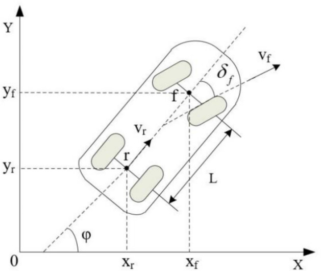
Vehicle kinematics model.
In the XOY coordinate system, represent vehicle rear axle center coordinates, represents the position of the front axle of the vehicle, and is the center speed of the rear wheel of the vehicle. is the yaw angle of the vehicle; is the equivalent Angle of the front wheel of the vehicle; l is the wheelbase. Combining the constraints of the rear axle with the speed of the rear axle yields the speed in the X and Y directions of the center of the rear axle.
| 1 |
Rear axle speed:
| 2 |
Simultaneity gives the velocity in the direction of the center of the rear axis:
| 3 |
Assuming the declination angle of the vehicle’s centroid remains constant during the steering process, which means that the instantaneous rotation radius of the vehicle is equal to the curvature radius of the road, we can combine Eqs. (2) and (3) as follows:
| 4 |
| 5 |
Finally, the yaw speed of the vehicle is obtained, and the formula is as follows:
| 6 |
The vehicle kinematics equation obtained is as follows:
| 7 |
Thus, the vehicle kinematics model of Ackermann steering is obtained. The model can be expressed in a general form:
| 8 |
where, state quantity , control quantity . From the above Eq. (7), it can be seen that the differential of the transverse and longitudinal coordinates of the vehicle is not integrable, and the driverless car must satisfy the nonholonomic constraint. Since the actuator restricts the front wheel to meet the limitation of the maximum steering Angle, the trajectory of the vehicle must meet the constraint of the maximum curvature, which is:
| 9 |
where is the minimum turning radius, is the maximum curvature, and is the maximum steering angle of the front wheel.
According to the kinematics model and the analysis of the front wheel’s maximum Angle, the planned path’s curvature should satisfy the constraint of the maximum Angle of the front wheel. Therefore, the steering process of the driverless car can only be described as a curve with continuous curvature and no more than the maximum curvature. Otherwise, the tracking control module cannot complete the accurate tracking of the path.
Related work
RRT algorithm
The RRT algorithm uses random sampling and rapid expansion to explore the search space. It randomly generates sampling points and expands the tree according to specific rules, gradually approaching the target point. Through iteration and connection, a feasible path from the initial point to the target point is finally found. The sampling method of RRT algorithm is shown in Fig. 2. The detailed step description of the algorithm are as follows:
Fig. 2.
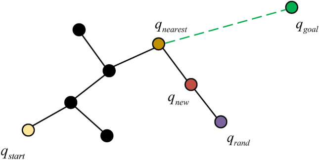
Sampling schematic diagram of the RRT* algorithm.
Initialize: Create and nodes.
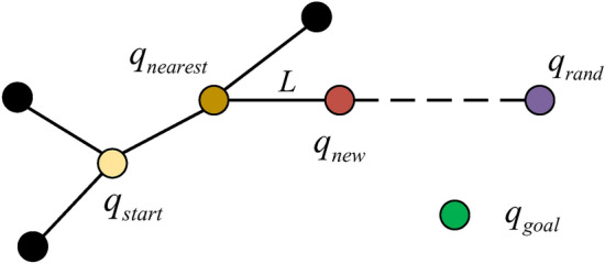
Tree growth: Randomly generate a node in the search space. Select the nearest node from the existing tree to . For the initial RRT sampling, set as . Then, generate a new node by extending from towards with a fixed step length L.
Obstacle detection: Check if there are obstacles between and . If there is an obstacle, discard the node and move on to the next sampling. Otherwise, add to the tree.
Goal connection: Check if the distance between and is less than the predefined threshold Thr. If so, connect to .
Repeat iterations: Iterate the above steps until a termination criterion is met (a certain number of iterations or a target configuration is reached).
Follow the path backward from the goal node to the start node to acquire the intended path.
The pseudocode representation of the algorithm is as follows:
Algorithm 1.

RRT.
The associated functions in the pseudo-code are described as follows:
Sample: Generates random points within the set environment
Nearest: Traverse the random tree to find the nearest node to the random point .
Steer: From the nearest node to the random point expand the random tree according to the set value to generate a new node .
Collsionfree: It detects whether there is an obstacle between two points.
T.addVertex: Insert a new node.
T.addEdge: Add an edge between and .
RRT* algorithm
RRT* algorithm is a progressive optimal path planning algorithm based on RRT. It improves existing paths through rewiring steps, shortens path segments through optimization steps, and takes node costs into account to generate high-quality and more optimized paths. Compared with RRT, RRT* has better path quality, because it can find a better path while ensuring search efficiency. RRT* is a variant of the RRT algorithm whose pseudo-code is shown in Algorithm 2.
Algorithm 2.

RRT*.
Some of the functions have the same definition and function as the RRT algorithm, and the new improved functions are described as follows:
Dist: Calculate the distance between two points.
Cost: Calculate the path cost from a given point along each edge of the random tree to the starting point.
The RRT* algorithm does not choose the nearest node as the parent node of the new node, but in a certain range around the new node, chooses the node with the best path (the least cost) as the parent node of the new node. As shown in Fig. 3, the method is to draw a circle around and compare the distance between a point in the circle and . If the distance between and is less than the distance between and or , and are connected. Meanwhile, we need to compare the shortest distance between and . If the distance between and is shorter, we update the parent of to . This step is called the reconnect.
Fig. 3.

RRT* algorithm expansion schematic.
Compared with RRT, the RRT* algorithm has the advantage of re-selecting nearby nodes and reconnecting extended nodes of random trees, inheriting the Probabilistic completeness of the RRT algorithm and making the planned routes more optimized. The RRT and RRT* algorithms have proven effective in numerous real-world scenarios such as robot motion planning, self-driving car navigation, and computer animation. Their efficiency and probabilistic nature render them highly adaptable to environments with intricate obstacles and high-dimensional configuration spaces. But as a cost, in the algorithm iteration after iteration, the process of solving requires a lot of memory; The algorithm suffers from extended execution time, sluggish convergence speed, and inadequate efficiency, presenting a prominent issue that requires attention.
Related improvement
In this section, we apply the variable probability goal-bias strategy to the RRT* algorithm to expedite the search for the target point. The APF method is enhanced and integrated into the RRT* algorithm framework to improve the quality and feasibility of the generated path.
Improved A-RRT* with variable probability goal-bias strategy
Improved A-RRT* with variable probability goal-bias strategy is a synthetic algorithm based on RRT*, APF, and variable probability target bias strategy. Firstly, a variable-probability goal-bias strategy is proposed in the step of the sampling process to expand the tree structure toward the target direction, improving the random tree’s sampling efficiency. Secondly, improvements are made to the potential field function in APF to prevent falling into local optimum problems during path generation. Thirdly, in the framework of RRT*, the improved APF method is integrated into the generation of new nodes, which makes the target point generate attraction and accelerates the expansion of the random tree towards the target direction. The pseudo-code of the algorithm is shown in Algorithm 3.
Algorithm 3.

Improved APF-RRT*.
The algorithm improves the artificial potential field, and the improved pseudo-code ImprovedAPF is shown in Algorithm 4.
Algorithm 4.

The associated functions in the pseudo-code are described as follows:
Mindistance: It refers to the distance from the nearest node to the center of the nearest obstacle circle at that point.
Generatenode: It refers to the function that generates the next new node under the action of the resultant force.
Variable probability goal-bias strategy
In the classic RRT* algorithm, the random tree expands through random sampling across the entire space to explore uncovered areas and eventually find a path to the target point. However, completely random sampling may lead to inefficiency in high-dimensional spaces, as the expansion of random trees lacks clear directionality, potentially wasting a significant amount of computational resources.
To improve sampling efficiency, the goal-bias strategy is introduced21. The basic idea of goal-bias strategy is to increase the probability of sampling points towards the target region, thereby guiding the random tree to expand more quickly towards the target point. In the initial stage, the sampling of RRT* is completely random, which allows for extensive exploration capabilities. However, due to the entirely random nature of initial RRT* sampling, its search in the sampling space is aimless, leading to low efficiency. By implementing goal biasing, the probability of sampling points selecting the target point can be increased, thereby promoting directed growth of the tree. The growth process of the random tree under the goal biasing strategy is shown in Fig. 4, and the calculation formula is shown in Eq. (10):
Fig. 4.
The goal-bias strategy leads to the growth of new nodes.
| 10 |
where rand() represents a random value ranging from 0 to 1, and P is the set goal probability threshold, which is used to determine the probability of selecting the target point during the sampling process. If the generated random number is less than the probability threshold, the target point is directly taken as the sampling point. Otherwise, according to the normal uniform distribution, a random point is generated in the search space as the sampling point.
The goal biasing strategy is an improved method that makes the algorithm more inclined to expand the tree toward the target region. However, in Goal-bias RRT*, the probability P of selecting the target point as the sampling point is fixed. When the random tree gets trapped in a local minimum, using the target point as the sampling point is generally ineffective, which can waste a significant amount of computational resources. The tendency to get trapped in local optima during sampling can be due to several factors:
High Goal Bias : If the goal bias is too high, the algorithm may prematurely abandon exploration of areas that appear to be far from the target, leading to local optima.
Inappropriate Sampling Strategy : The sampling strategy should balance global and local exploration to ensure sufficient diversity in the search space. If sampling is too concentrated in certain areas, it may lead to local optima.
Difficult-to-Reach Target Areas : If the target area contains obstacles or narrow paths, the goal-bias strategy might cause the algorithm to focus too much on these hard-to-reach areas, hindering effective exploration of other possible paths.
To address this, this paper proposes a variable probability sampling method, which introduces a certain degree of randomness in the tree expansion process. By dynamically adjusting the probability of selecting the target point as the sampling point, the algorithm’s efficiency is improved, preventing it from becoming overly concentrated in local areas. Specifically, this strategy uses a probability threshold P to decide whether to choose a random point or the target point as the sampling point. When a random number (between 0 and 1) is greater than P, a random point is selected as the sampling point; otherwise, the target point is chosen.
The core of the variable probability goal-bias strategy lies in how to dynamically adjust the probability value P. This paper proposes an adjustment formula based on the number of growth iterations:
| 11 |
where is the probability of selecting the target point as the sampling point at the initial time, is the form factor, is the maximum number of attempts set. n is the current number of random increases.
The value of P is dynamically adjusted based on the progress of the algorithm. Initially, P is set to a fixed value, allowing the random tree to fully explore the surrounding space and avoid prematurely falling into local optima. When expanding by selecting the target point as the sampling point proves ineffective, it can be assumed that the random tree is trapped in a local minimum. At this point, P is set to 0, allowing the algorithm to focus on escaping the local minimum through random growth. As the number of random growth iterations increases, the likelihood of the random tree escaping the local minimum also increases. Consequently, the value of P is gradually increased, which raises the probability of goal bias, allowing the tree to grow more towards the target point.
The improved APF algorithm
In order to ensure the real-time performance of vehicle path planning in practical applications, we utilized APF algorithm. Based on RRT* algorithm, an improved APF method is added to enhance the generation of new point and improve the quality of the generated path. APF method consists of two key parts: gravitational potential field and the repulsion potential field . These components are represented by Eqs. (12) and (13), respectively.
| 12 |
| 13 |
where and are the gravitational potential field constant and the repulsive potential field constant, is the radius of influence of the repulsive potential field, and respectively the trajectory point q to target and recent obstacles Euclidean distance.
The gravitational of the vehicle in the gravitational potential field and the repulsive in the repulsive potential field are shown in Eqs. (14) and (15):
| 14 |
| 15 |
When an obstacle approaches a target point, the attraction of the target point to the vehicle may be less than the repulsive force of the obstacle to the vehicle, resulting in an unreachable target problem. In addition, when the gravitational and repulsive forces acting on the vehicle are equal in magnitude, a state of force equilibrium occurs and the vehicle comes to a standstill.
To solve this problem, a new repulsion function can be introduced, that is, based on the original repulsion potential field function, the influence of the distance between the target and the vehicle is added. When the vehicle is near the obstacle, although the repulsive force of the vehicle is increasing, the distance between the vehicle and the obstacle is decreasing, so the increase in the distance reduces the repulsive potential field to a certain extent, which is equivalent to the role of dragging the repulsive force field, which can effectively drag the vehicle to the target position. The new repulsive field function is expressed as:
| 16 |
where and are the positions of and obstacles, is the distance from to , is the distance from to , is the distance from to the nearest obstacle. The corresponding repulsive force is:
| 17 |
| 18 |
| 19 |
where and are the direction vectors from the nearest obstacle to and to , n is a positive integer.
In the RRT* algorithm framework, the vehicle is subjected to the gravitational force under the joint action of target points and random points, and the new gravitational potential field is:
| 20 |
| 21 |
| 22 |
The corresponding gravitational force is:
| 23 |
| 24 |
As the vehicle moves towards the target point, the vehicle will be subjected to the combined action of the attractive potential field and the repulsive potential field. The force on the vehicle is:
| 25 |
where and respectively is and to , is the repulsive force of the nearest obstacle to . The resultant force is obtained from the parallelogram rule, and new nodes are generated in the resultant direction. The stress diagram of is shown in Fig. 5. These forces determine the direction and strength of the effect on the driverless car. By combining these equations and variables, the system can effectively generate an attraction to the target point while keeping the car away from obstacles, thus making the driverless car safe to drive.
Fig. 5.
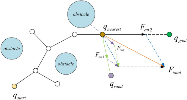
The force analytical graph of .
Experimental simulation
The simulations were conducted using MATLAB 2016b. The simulation results of RRT*17, the goal-bias RRT* algorithm (G-RRT*)21, the GPF-RRT* algorithm29, the APF-IRRT*30 algorithm, the H-RRT* algorithm, and the Improved A-RRT* algorithm were compared to demonstrate the advantages of the Improved A-RRT* algorithm in terms of faster convergence speed and shorter path length. The simulation environment consists of a 2D space with a map size of 1000*1000. The starting point is at coordinates (0,0), and the goal point is at coordinates (1000,1000). The starting and goal points are represented in pink and blue, respectively. For G-RRT*, GPF-RRT*, and Improved A-RRT* algorithms, the goal-bias probability P is set to 0.2. For APF-IRRT*, GPF-RRT*, and Improved A-RRT* algorithms, the attraction coefficient , the repulsion coefficient , the connection threshold is 20, and the step size is 20. The obstacle positions in the simulation environment are the same for all algorithms. Data from 100 trials in different environments were used to analyze and compare the different algorithms. Figure 6 shows the five experimental settings: Environment A, Environment B, Environment C, Environment D, and Environment E. The deep purple objects on the map represent obstacles that the autonomous vehicle cannot pass through.
Fig. 6.

Experimental environment.
Environment A
In Environment A, each algorithm was compared based on 100 simulations of path length, search time, and number of path nodes, under the same conditions, the simulation results are shown in Fig. 7. Based on 100 experimental data points, the average trajectory length of the proposed algorithm was 1532.9, the average runtime was 3.4109, and the average number of path nodes was 50.40. As shown in Table 1 and Fig. 8, the average path length of the Improved A-RRT* algorithm was approximately 13.35% shorter than that of the RRT* algorithm, 9.91% shorter than the G-RRT* algorithm, 3.35% shorter than the GPF-RRT* algorithm, 4.26% shorter than the APF-IRRT* algorithm, and 15.40% shorter than the H-RRT* algorithm. This improvement is attributed to the introduction of the variable probability goal-bias strategy during the tree node growth process, as well as the incorporation of an enhanced artificial potential field function, which improves path quality.
Fig. 7.

Simulation in environment A.
Table 1.
Simulation data in environment A.
| Algorithms | Mean path length (m) | Mean running time (s) | Mean number of nodes |
|---|---|---|---|
| RRT* | 1769.0 | 14.4022 | 65.90 |
| G-RRT* | 1701.6 | 5.3758 | 63.65 |
| GPF-RRT* | 1586.0 | 3.8012 | 52.35 |
| APF-IRRT* | 1601.1 | 9.2507 | 55.60 |
| H-RRT* | 1811.8 | 1.5524 | 25.45 |
| Improved A-RRT* | 1532.9 | 3.4109 | 50.40 |
Fig. 8.

Data comparison diagram in environment A.
The average runtime of the Improved A-RRT* algorithm was 78.19% shorter than the RRT* algorithm, 36.55% shorter than the G-RRT* algorithm, approximately 10.27% shorter than the GPF-RRT* algorithm, and 63.13% shorter than the APF-IRRT* algorithm, making the Improved A-RRT* algorithm faster than the other four algorithms and demonstrating its effectiveness. Regarding the average number of nodes (all nodes on the final path when the iteration stops), the Improved A-RRT* algorithm had 30.75% fewer nodes than the RRT* algorithm, 20.82% fewer than the G-RRT* algorithm, approximately 3.87% fewer than the GPF-RRT* algorithm, and about 10.32% fewer than the APF-IRRT* algorithm.
This is due to the fact that the Improved A-RRT* algorithm terminates iterations at an earlier stage, resulting in a significantly reduced number of nodes in the tree in comparison to other algorithms. Despite the H-RRT* algorithm having the shortest average search time and the fewest nodes, the quality of the generated paths was inferior, and the paths were less smooth. Consequently, in the map A environment, the Improved A-RRT* algorithm demonstrates superior performance in comparison to the other algorithms.
Environment B
Compared to Environment A, the obstacles in Environment B are more closely spaced, making it difficult to plan a smooth and passable path. To demonstrate the superior performance of the proposed algorithm, we conducted 100 experiments for each algorithm in Environment B, recording the runtime, generated path length, and the number of path nodes. The simulation results of the three algorithms are shown in Fig. 9, and the experimental data are presented in Table 2 and Fig. 10. The average path length of the proposed algorithm is 1601.4, the average runtime is 4.6781, and the average number of path nodes is 51.55. Compared to the RRT*, G-RRT*, GPF-RRT*, and APF-IRRT* algorithms, the average runtime of the proposed algorithm is reduced by 69.10%, 38.64%, 21.09%, and 69.17%, respectively. The average path length and the average number of nodes are reduced by 12.47%, 9.43%, 6.05%, 6.99%, and 24.63%, 20.08%, 6.70%, 10.50%, respectively. The H-RRT* algorithm uses the distance between the target point and the random point as a heuristic value, which allows the algorithm to develop more quickly towards the target direction, significantly improving search time efficiency. However, the accuracy of its heuristic function needs improvement, leading to a decline in path quality.
Fig. 9.

Simulation in environment B.
Table 2.
Simulation data in environment B.
| Algorithms | Mean path length (m) | Mean running time (s) | Mean number of nodes |
|---|---|---|---|
| RRT* | 1829.6 | 15.1384 | 68.40 |
| G-RRT* | 1768.1 | 7.6246 | 64.50 |
| GPF-RRT* | 1704.6 | 5.9282 | 55.25 |
| APF-IRRT* | 1721.8 | 15.1754 | 57.60 |
| H-RRT* | 1980.8 | 2.6009 | 26.90 |
| Improved A-RRT* | 1601.4 | 4.6781 | 51.55 |
Fig. 10.

Data comparison diagram in environment B.
As shown in Fig. 9a, in this environment, the RRT* algorithm covers a large area of sampling nodes across the entire map to find an initial solution, while the G-RRT*, GPF-RRT*, and Improved A-RRT* algorithms can find paths with fewer nodes. The latter two algorithms optimize the sampling pattern using the goal-bias strategy, speeding up path generation. Compared to the G-RRT* algorithm, the GPF-RRT*, APF-IRRT*, and Improved A-RRT* algorithms introduce the APF algorithm, resulting in higher path quality. Due to the optimization of the goal-bias strategy into a variable probability goal-bias strategy in the Improved A-RRT* algorithm, it achieves faster convergence speed. As shown in Fig. 9f, under the influence of the goal point’s gravitational force, the path segments without obstacles between the path nodes and the goal are smoother, and fewer nodes are required to generate the path. Therefore, in the environment B, the performance of the Improved A-RRT* algorithm is superior to that of the other two algorithms.
Environment C
Compared to Environment A and B, Environment C has more obstacles, which are distributed in various locations across the map. As shown in Fig. 11, the RRT algorithm generates a large number of redundant points during the growth of the random tree, resulting in rough paths and longer search times. The G-RRT algorithm introduces a goal biasing strategy, which reduces search time but results in lower path quality. Figure 11c and d show that the introduction of the APF (Artificial Potential Field) improves the quality of the generated paths. Figure 11f illustrates that in the Improved A-RRT* algorithm, the sampling and growth process of the random tree tends more towards the direction from the starting point to the goal point, reducing the number of nodes required to obtain a path. At the same time, under the influence of the variable Probability goal-bias strategy, the convergence speed of the algorithm is significantly improved.
Fig. 11.

Simulation in environment C.
From Table 3 and Fig. 12, it can be seen that in Environment C, the average path length of the initial solutions generated from 100 experiments is 1450.9, the average runtime is 3.1203, and the average number of path nodes is 49.00. In terms of average path length, the Improved A-RRT* algorithm is approximately 18.31% shorter than the RRT* algorithm, 12.50% shorter than the G-RRT* algorithm, 4.76% shorter than the GPF-RRT* algorithm, 6.29% shorter than the APF-IRRT* algorithm, and 25.67% shorter than the H-RRT* algorithm. The average runtime of the Improved A-RRT* algorithm is reduced by 74.08% compared to the RRT* algorithm, 42.73% compared to the G-RRT* algorithm, approximately 21.09% compared to the GPF-RRT* algorithm, and 69.17% compared to the APF-IRRT* algorithm. Regarding the average number of nodes, the Improved A-RRT* algorithm uses 26.81% fewer nodes than the RRT* algorithm, 21.54% fewer than the G-RRT* algorithm, approximately 6.70% fewer than the GPF-RRT* algorithm, and about 10.50% fewer than the APF-IRRT* algorithm. By comparing 100 sets of data, the proposed algorithm achieves significant improvements in all three performance metrics, including reduced path length, shortened runtime, and fewer path nodes.
Table 3.
Simulation data in environment C.
| Algorithms | Mean path length (m) | Mean running time (s) | Mean number of nodes |
|---|---|---|---|
| RRT* | 1776.1 | 12.0365 | 66.95 |
| G-RRT* | 1658.2 | 5.4488 | 62.45 |
| GPF-RRT* | 1523.4 | 4.4112 | 56.25 |
| APF-IRRT* | 1548.3 | 10.8273 | 56.70 |
| H-RRT* | 1951.9 | 2.7997 | 27.30 |
| Improved A-RRT* | 1450.9 | 3.1203 | 49.00 |
Fig. 12.

Data comparison diagram in environment C.
Environment D
This section uses simulation experiments with a narrow road intersection obstacle map, with the simulation paths of each algorithm shown in Fig. 13. The relevant data generated from the experiments are shown in Fig. 14 and Table 4. As seen in Fig. 14 and Table 4, the Improved A-RRT* algorithm has an average search time that is approximately 79.52% shorter than the RRT* algorithm, 30.81% shorter than the G-RRT* algorithm, 22.32% shorter than the GPF-IRRT* algorithm, 76.07% shorter than the APF-IRRT* algorithm, and 67.20% shorter than the H-RRT* algorithm, demonstrating the efficiency of the Improved A-RRT* algorithm.
Fig. 13.

Simulation in environment D.
Fig. 14.

Data comparison diagram in environment D.
Table 4.
Simulation data in environment D.
| Algorithms | Mean path length (m) | Mean running time (s) | Mean number of nodes |
|---|---|---|---|
| RRT* | 1568.1 | 14.3724 | 60.75 |
| G-RRT* | 1499.0 | 4.2548 | 53.75 |
| GPF-RRT* | 1502.6 | 3.7893 | 54.00 |
| APF-IRRT* | 1556.7 | 12.3027 | 56.20 |
| H-RRT* | 1753.4 | 8.9735 | 25.95 |
| Improved A-RRT* | 1446.9 | 2.9437 | 50.85 |
As shown in Fig. 13c, the number of sampling points on the left side for each algorithm is significantly greater than on the right side. The next sampling point in the RRT* algorithm’s random sampling range is in the global map, which greatly reduces the ability of the random tree to pass through narrow areas. Therefore, the search efficiency of the basic RRT* algorithm is significantly reduced in narrow exit environments. The proposed algorithm uses a variable probability goal-bias strategy, guiding the random tree to grow towards the goal more efficiently through the narrow exit.
In terms of average path length, the Improved A-RRT* algorithm’s average path length is 7.73% shorter than that of the RRT* algorithm, 3.48% shorter than the G-RRT* algorithm, 3.71% shorter than the GPF-IRRT* algorithm, 7.05% shorter than the APF-IRRT* algorithm, and 17.48% shorter than the H-RRT* algorithm. Regarding the average number of nodes, the Improved A-RRT* algorithm has 16.30% fewer nodes than the RRT* algorithm, 5.40% fewer than the G-RRT* algorithm, 6.02% fewer than the GPF-IRRT* algorithm, and 9.52% fewer than the APF-IRRT* algorithm. The introduction of the APF algorithm results in an improvement in path quality and a reduction in the number of nodes required to generate the path in the Improved A-RRT* algorithm. Consequently, the Improved A-RRT* algorithm demonstrates superior performance compared to the other three algorithms in the narrow road intersection environment.
Environment E
This section uses simulation experiments with a continuous narrow passage obstacle map. The simulation paths for each algorithm are shown in Fig. 15. The relevant data generated from the experiments are shown in Fig. 16 and Table 5. Under the same iteration count of 5000, the H-RRT* algorithm fails to find a path in this environment. As shown in the figures, the paths generated by the proposed algorithm are shorter, smoother in quality, and have shorter search times, demonstrating the effectiveness of the algorithm.
Fig. 15.

Simulation in environment E.
Fig. 16.

Data comparison diagram in environment E.
Table 5.
Simulation data in environment E.
| Algorithms | Mean path length (m) | Mean running time (s) | Mean number of nodes |
|---|---|---|---|
| RRT* | 1742.4 | 30.2014 | 66.05 |
| G-RRT* | 1688.3 | 14.6520 | 58.85 |
| GPF-RRT* | 1623.2 | 13.8853 | 52.65 |
| APF-IRRT* | 1710.9 | 23.3191 | 77.85 |
| H-RRT* | – | – | – |
| Improved A-RRT* | 1609.0 | 6.2873 | 52.15 |
From Fig. 16 and Table 5, it can be seen that, in terms of average search time, the Improved A-RRT* algorithm is approximately 79.18% faster than the RRT* algorithm, 57.09% faster than the G-RRT* algorithm, 54.72% faster than the GPF-IRRT* algorithm, and 57.76% faster than the APF-IRRT* algorithm, confirming the efficiency of the Improved A-RRT* algorithm. This is due to the fact that the enhanced A-RRT* algorithm employs a variable probability goal-bias strategy, thereby introducing a certain degree of randomness during the expansion of the tree. Furthermore, the probability of selecting the target point as the sampling point is dynamically adjusted in order to enhance the efficiency of the algorithm and to prevent the algorithm from becoming overly concentrated in local areas.
In terms of average path length, the Improved A-RRT* algorithm’s average path length is 7.66% shorter than the RRT* algorithm, 4.70% shorter than the G-RRT* algorithm, 0.87% shorter than the GPF-IRRT* algorithm, and 5.96% shorter than the APF-IRRT* algorithm. Regarding the average number of nodes, the Improved A-RRT* algorithm uses 21.04% fewer nodes than the RRT* algorithm, 11.38% fewer than the G-RRT* algorithm, 0.95% fewer than the GPF-IRRT* algorithm, and 33.01% fewer than the APF-IRRT* algorithm. The incorporation of attraction and repulsion functions from the artificial potential field method within the Improved A-RRT* algorithm enables the guidance of the path towards the target direction. This is achieved by utilising the attraction from the goal point and the repulsion from obstacles, which improves the quality of the path.
Physics experiments
The experimental results in section “Experimental simulation” show that the Improved A-RRT* algorithm performs the best among all algorithms. The reason is that Eq. (10) can limit the generation range of random sampling points based on the position information of the target point, thereby reducing the number of iterations. Equation (11) can prevent the algorithm from falling into local optima under this strategy, and when one branch falls into a dead zone, other branches still have the opportunity to continue growing, thus improving the search efficiency of the random tree. Applying the Improved A-RRT* to the node , attraction to the random tree is introduced at the target and random points, and repulsion is introduced at obstacles, guiding the generation of new nodes .
Compared to the global sampling of the RRT* algorithm, the paths generated by the Improved A-RRT* algorithm are smoother, and the runtime is shorter. Compared to the G-RRT* algorithm, the proposed algorithm, due to its use of the variable probability goal-bias strategy, is more effective in finding paths in complex narrow road environments. The H-RRT* algorithm, by incorporating heuristic functions from the A* algorithm, introduces the distance between the target point and the random point as a heuristic value in the selection of new nodes, guiding the generation of paths that are closer to the target. Although the H-RRT* algorithm finds paths more quickly, the quality of the generated paths is rough, and there are instances of search path failure in more complex continuous narrow road environments.
Compared to the GPF-IRRT* and APF-IRRT* algorithms, the Improved A-RRT* algorithm, by employing the variable probability goal-bias strategy, more easily expands towards the target direction, finds feasible solutions more quickly, and reduces the search space. The introduction of the APF makes the generated paths more direct and efficient, reducing the number of redundant nodes. Since both the goal-bias strategy and the APF method optimize the quality of path planning, the Improved A-RRT* algorithm can generate better paths with higher passability and safety.
Conclusion
This paper introduces a new path planning algorithm for autonomous vehicles, the Improved A-RRT* algorithm. This algorithm incorporates a variable probability goal-bias strategy into the sampling process of the RRT* algorithm, thereby increasing the likelihood of selecting the goal as a sampling point. This enhances the expansion of new nodes towards the goal direction and significantly improves the search efficiency of the random tree. After generating the nearest node, the algorithm incorporates an enhanced artificial potential field method. The vehicle is influenced by the repulsive force from the nearest obstacle node while simultaneously being attracted by the random point and the goal point, which significantly boosts the search performance of the algorithm.
Simulation results demonstrate that the Improved A-RRT* algorithm performs excellently in various complex environments, including narrow passages and scenarios with densely distributed obstacles. While ensuring good path quality and obstacle avoidance capabilities, the algorithm effectively accelerates convergence speed and reduces the occurrence of redundant points. Although this algorithm excels in terms of speed and efficiency, it may involve certain trade-offs in path smoothness and optimality in some scenarios, particularly when compared with algorithms specifically designed to optimize path quality.
Future research will focus on enhancing the adaptability of this algorithm in more complex environments. This includes further investigations into the performance of autonomous vehicles in complex dynamic environments and exploring effective maneuvering and obstacle avoidance strategies to achieve more reliable and safer trajectory planning.
Acknowledgements
This work was supported in part by the National Natural Science Foundation of China under Grant (62301212,62371182,62401240), the Program for Science and Technology Innovation Talents in the University of Henan Province under Grant (23HASTIT021), Major Science and Technology Projects of Longmen Laboratory under Grant (231100220300), the Key Scientific Research Projects of Universities in Henan Province (25A413001).
Author contributions
All authors contributed to the study’s conception and design. Material preparation and data collection were performed by F.Z.. The first draft of the manuscript was written by D.Z. and T.F. guided the writing process. L.M. helped improve the experiments. J.B. helped with the formatting review and editing of the paper. All authors read and approved the final manuscript.
Data availability
The datasets generated and analysed during the current study are not publicly available due Laboratory confidentiality policy but are available from the corresponding author on reasonable request.
Conflict of interest
The authors declare that they have no conflict of interest.
Footnotes
Publisher’s note
Springer Nature remains neutral with regard to jurisdictional claims in published maps and institutional affiliations.
References
- 1.Verma, S., Kaur, S., Sharma, A. K., Kathuria, A. & Piran, M. J. Dual sink-based optimized sensing for intelligent transportation systems. IEEE Sens. J. 21(14), 15867–15874 (2020). [Google Scholar]
- 2.Claussmann, L., Revilloud, M., Gruyer, D. & Glaser, S. A review of motion planning for highway autonomous driving. IEEE Trans. Intell. Transp. Syst. 21(5), 1826–1848 (2019). [Google Scholar]
- 3.Rasekhipour, Y., Fadakar, I. & Khajepour, A. Autonomous driving motion planning with obstacles prioritization using lexicographic optimization. Control. Eng. Pract. 77, 235–246 (2018). [Google Scholar]
- 4.Liu, L. et al. Path planning techniques for mobile robots: Review and prospect. Expert Syst. Appl. 2023, 120254 (2023). [Google Scholar]
- 5.Paden, B., Čáp, M., Yong, S. Z., Yershov, D. & Frazzoli, E. A survey of motion planning and control techniques for self-driving urban vehicles. IEEE Trans. Intell. Veh. 1(1), 33–55 (2016). [Google Scholar]
- 6.Liu, L.-S. et al. Path planning for smart car based on dijkstra algorithm and dynamic window approach. Wirel. Commun. Mob. Comput. 2021, 1–12 (2021).35573891 [Google Scholar]
- 7.Prasad, N. L. & Ramkumar, B. 3-d deployment and trajectory planning for relay based uav assisted cooperative communication for emergency scenarios using dijkstra’s algorithm. IEEE Trans. Veh. Technol. 72(4), 5049–5063 (2022). [Google Scholar]
- 8.Zhang, Z., Jiang, J., Wu, J. & Zhu, X. Efficient and optimal penetration path planning for stealth unmanned aerial vehicle using minimal radar cross-section tactics and modified a-star algorithm. ISA Trans. 134, 42–57 (2023). [DOI] [PubMed] [Google Scholar]
- 9.Meng, T. et al. Improved hybrid a-star algorithm for path planning in autonomous parking system based on multi-stage dynamic optimization. Int. J. Automot. Technol. 24(2), 459–468 (2023). [Google Scholar]
- 10.Han, G. et al. Ant-colony-based complete-coverage path-planning algorithm for underwater gliders in ocean areas with thermoclines. IEEE Trans. Veh. Technol. 69(8), 8959–8971 (2020). [Google Scholar]
- 11.Chen, Z. et al. An effective path planning of intelligent mobile robot using improved genetic algorithm. Wirel. Commun. Mobile Comput. 2022, 569 (2022). [Google Scholar]
- 12.Zhai, L. & Feng, S. A novel evacuation path planning method based on improved genetic algorithm. J. Intell. Fuzzy Syst. 42(3), 1813–1823 (2022). [Google Scholar]
- 13.Lin, S., Liu, A., Wang, J. & Kong, X. An intelligence-based hybrid pso-sa for mobile robot path planning in warehouse. J. Comput. Sci. 67, 101938 (2023). [Google Scholar]
- 14.Yu, Z., Si, Z., Li, X., Wang, D. & Song, H. A novel hybrid particle swarm optimization algorithm for path planning of uavs. IEEE Internet Things J. 9(22), 22547–22558 (2022). [Google Scholar]
- 15.LaValle, S. M., & Kuffner, J. J. Rapidly-exploring random trees: Progress and prospects: Steven m. In lavalle, iowa state university, a james j. kuffner, jr., university of tokyo, tokyo, japan, Algorithmic and computational robotics 303–307 (2001).
- 16.LaValle, S. Rapidly-exploring random trees: A new tool for path planning, Research Report 9811 (1998).
- 17.Karaman, S. & Frazzoli, E. Sampling-based algorithms for optimal motion planning. Int. J. Robot. Res. 30(7), 846–894 (2011). [Google Scholar]
- 18.Gammell, J. D., Srinivasa, S. S., & Barfoot, T. D. Informed rrt*: Optimal sampling-based path planning focused via direct sampling of an admissible ellipsoidal heuristic 2997–3004 (2014).
- 19.Nasir, J. et al. Rrt*-smart: A rapid convergence implementation of rrt. Int. J. Adv. Rob. Syst. 10(7), 299 (2013). [Google Scholar]
- 20.Tak, H.-T., Park, C.-G. & Lee, S.-C. Improvement of rrt*-smart algorithm for optimal path planning and application of the algorithm in 2 & 3-dimension environment. J. Korean Soc. Aviation Aeronaut. 27(2), 1–8 (2019). [Google Scholar]
- 21.Urmson, C., & Simmons, R. Approaches for heuristically biasing rrt growth. In Proceedings 2003 IEEE/RSJ International Conference on Intelligent Robots and Systems (IROS 2003) (Cat. No. 03CH37453), Vol. 2 1178–1183 (IEEE, 2003).
- 22.Kim, M., Ahn, J. & Park, J. Targettree-rrt*: Continuous-curvature path planning algorithm for autonomous parking in complex environments. IEEE Trans. Autom. Sci. Eng. 2022, 56 (2022). [Google Scholar]
- 23.Wang, J., Li, T., Li, B. & Meng, M.Q.-H. Gmr-rrt*: Sampling-based path planning using gaussian mixture regression. IEEE Trans. Intell. Veh. 7(3), 690–700 (2022). [Google Scholar]
- 24.Wang, J., Chi, W., Li, C., Wang, C. & Meng, M.Q.-H. Neural rrt*: Learning-based optimal path planning. IEEE Trans. Autom. Sci. Eng. 17(4), 1748–1758 (2020). [Google Scholar]
- 25.Chao, N., Liu, Y.-K., Xia, H., Peng, M.-J. & Ayodeji, A. Dl-rrt* algorithm for least dose path re-planning in dynamic radioactive environments. Nucl. Eng. Technol. 51(3), 825–836 (2019). [Google Scholar]
- 26.Pradhan, S., Mandava, R. K. & Vundavilli, P. R. Development of path planning algorithm for biped robot using combined multi-point rrt and visibility graph. Int. J. Inf. Technol. 13(4), 1513–1519 (2021). [Google Scholar]
- 27.Guo, Y., Liu, X., Jia, Q., Liu, X. & Zhang, W. Hpo-rrt*: A sampling-based algorithm for uav real-time path planning in a dynamic environment. Complex Intell. Syst. 9(6), 7133–7153 (2023). [Google Scholar]
- 28.Cong, J. et al. Ff-rrt*: A sampling-improved path planning algorithm for mobile robots against concave cavity obstacle. Complex Intell. Syst. 9(6), 7249–7267 (2023). [Google Scholar]
- 29.Fan, J., Chen, X., Wang, Y. & Chen, X. Uav trajectory planning in cluttered environments based on pf-rrt* algorithm with goal-biased strategy. Eng. Appl. Artif. Intell. 114, 105182 (2022). [Google Scholar]
- 30.Wu, D., Wei, L., Wang, G., Tian, L. & Dai, G. Apf-irrt*: An improved informed rapidly-exploring random trees-star algorithm by introducing artificial potential field method for mobile robot path planning. Appl. Sci. 12(21), 10905 (2022). [Google Scholar]
Associated Data
This section collects any data citations, data availability statements, or supplementary materials included in this article.
Data Availability Statement
The datasets generated and analysed during the current study are not publicly available due Laboratory confidentiality policy but are available from the corresponding author on reasonable request.