Buffed energy landscapes: Another solution to the kinetic paradoxes of protein folding

Abstract

The energy landscapes of proteins have evolved to be different from most random heteropolymers. Many studies have concluded that evolutionary selection for rapid and reliable folding to a given structure that is stable at biological temperatures leads to energy landscapes having a single dominant basin and an overall funnel topography. We show here that, although such a landscape topography is indeed a sufficient condition for folding, another possibility also exists, giving a previously undescribed class of foldable sequences. These sequences have landscapes that are only weakly funneled in the conventional thermodynamic sense but have unusually low kinetic barriers for reconfigurational motion. Traps have been specifically removed by selection. Here we examine the possibility of folding on these “buffed” landscapes by mapping the determination of statistics of pathways for the heterogeneous nucleation processes involved in escaping from traps to the solution of an imaginary time Schroedinger equation. This equation is solved analytically in adiabatic and “soft-wall” approximations, and numerical results are shown for the general case. The fraction of funneled vs. buffed proteins in sequence space is estimated, suggesting the statistical dominance of the funneling mechanism for achieving foldability.

The mechanisms of protein folding are manifold. This diversity can only be captured by a global statistical survey of the protein's energy landscape. What can be said about this landscape merely from the knowledge that proteins fold?

A foldable protein is a heteropolymer that through Brownian motion finds a particular structure within a short time and, once this structure is found, essentially stays in that structure. This requirement is both thermodynamic and kinetic. Thermodynamically, the folded state of a protein must be stable and tolerably unique. Although conformational substrates can be functionally important and are decidedly present (1), the specificity of proteins required for their work in the cellular network leads to strong constraints on the structure of the active sites and binding sites of proteins.

For random heteropolymers, thermodynamic foldability depends on the relation between the physiological temperature and the glass temperature, which depends on the amino acid composition. For some compositions, e.g., near homopolymers, T_G is low, whereas for other compositions using many chemically distinct amino acids, T_G could be higher than physiological temperatures. If physiological temperatures are very high, only a small fraction of all sequences will be foldable in a thermodynamic sense, because few sequences would have sufficient stability in the ground-state conformation against entropic costs. At sufficiently low temperatures, all sequences would have stable ground states, providing the solvent is such that interaction-free energies do not change much as temperature is lowered. But in this low-temperature case, the kinetics of folding would become the controlling factor. For a typical random sequence of amino acids, while the lowest energy state becomes thermodynamically stable only below the glass transition temperature T_G, at these low temperatures several other traps will also become stable. The average escape time from these traps scales exponentially in chain length. Thus for long enough chains folding will be slow.

One resolution of this conflict between kinetic and thermodynamic constraints is for proteins to have evolved to have compositions with T_G < T but to be unusual sequences that nevertheless are stable in some configuration above T_G via the introduction of an energy gap in the density of states such that one energetic basin dominates. The energy landscape is funneled, with a single dominant basin (2). According to this view, proteins are atypical heteropolymers by having their folding transition temperature T_F above the glass temperature T_G to be expected ordinarily from the overall amino acid composition. This is the quantitative form of the principle of minimal frustration that was put forward by Bryngelson and Wolynes (3).

An extreme limit of the principle of minimal frustration would be for there to exist perfect consistency of interactions in the native state, an idea due to Gō and coworkers (4). In the space of all sequences, such perfection is less likely than merely achieving a satisfactory level of resolved frustration. Most microscopic potential models suggest that natural proteins still exhibit frustration in their ground state. The existence of this frustration is buttressed by the observation that many proteins can be stabilized further by single site mutations. Nevertheless, the perfect funnel model does describe the kinetics of folding of many proteins as a first approximation, as seen by the good agreement of φ values predicted by using Gō models with experiments (refs. 5–7 and references therein).

The iconoclasts among us, nevertheless, must ask whether the achievement of a funneled landscape with T_F/T_G > 1 is the only way the kinetic/thermodynamic requirements for folding can be met. Rather than finding sequences that increase the native stability under conditions where dynamics of a random sequence would be facile, we can imagine designing an abnormally trap-free landscape giving unusually high mobility throughout the misfolded parts of the energy landscape.

In this case, heteropolymers having compositions giving T_G > T would easily have a ground state that is stable, but it would be necessary to design out the barriers for escaping the deep traps such that those barriers were atypically small. The density of low-energy states would not be atypical in this case; rather, what is atypical is the size of the kinetic barriers between the states. Such an energy landscape could be said to be “buffed.” Even on such a buffed energy landscape, the native state still must have some extra stability to avoid the time-scale problems of a random search. But the extra stability in this scenario need not scale extensively with system size and may scale as a nonextensive fluctuation ∼ N^1/2 or smaller.

It is intriguing that some of the successes of theories based on the strongly funneled landscape would be preserved for theories based on buffed landscapes. For example, because the ruggedness en route to the native structure is reduced and the effects of transient trapping diminished, native structure formation (as measured through φ values) will once again be dominated by polymeric properties. However, there should be observable differences between buffed and funneled landscapes in stability and robustness. The native state on a funneled landscape is marginally stable with respect to a large ensemble of unfolded states having significant entropy. The native state on a buffed landscape is marginally stable with respect to a few dissimilar low-energy states that are kinetically connected to it. Thus the thermal unfolding transition on a buffed landscape should be less cooperative than on a funneled landscape. The folded structure and folding mechanism are also less robust on a buffed landscape, because mutations can more easily open up or close off regions of searchable phase space. These differences between the properties expected for buffed sequences and natural proteins suggest that natural protein landscapes mainly are funneled rather than buffed.

Yet given the possibility of having a buffed energy landscape, the explanation for the prevalence of funneled landscapes must be sought in statistics and population biology (8). The question we address is whether the fraction of sequences with buffed landscapes is comparable or larger than the fraction of sequences with minimally frustrated landscapes in the conventional sense. This is the task of the present article.

Nucleation

Both folding and trap escape can be thought of as the growth of a new phase into a preexisting phase. This growth requires overcoming a barrier of finite height. According to classical nucleation theory, we can introduce a reaction coordinate N_e describing the amount of new phase, 0 ≤ N_e ≤ N, where N is the length of the chain. The typical free-energy profile as a function of N_e is

Here f is the bulk free-energy gain per residue in the new phase, and σ is the surface free-energy cost per residue. These parameters are each a function of temperature.

For a uniformly stable phase, the exponent z = 2/3. However, in a sufficiently heterogeneous medium the interface between phases can relax to a lower free-energy configuration that is roughened. The larger the nucleus, the more the interface can relax and the smaller the surface tension. For a wide class of models in three dimensions in this regime (9, 10), σ = σ_o/N, and the surface free-energy cost scales as N rather than N. This is also true for a random first-order glass transition.

Setting ∂F̄(N_e)/∂N_e = 0 gives the typical critical nucleus size, N̄ ≡ Nn̄ = (zσ/f)^1/(1−z), where 0 ≤ n_F ≤ 1. The typical free-energy barrier height is

Thus the barrier arises from surface cost and scales as N^z.

Generally for glassy systems at high enough temperature, trap escape becomes a downhill process, corresponding to a vanishing of the surface tension in the nucleation picture.

Atypically Rugged and Funneled Sequences

Suppose each amino acid was chosen from a pool with probability p for residue type i, where 1 < i < m with m = 20 and ∑_i p = 1. Shorter sequences may have compositions with probabilities of occurrence {p_i} differing from {p}, but as the chain length increases, p_i approaches p. The probability of a composition {n_i}, 0 ≤ n_i ≤ N, chosen randomly from a pool with natural abundances {p} is given by a multinomial distribution. We are interested in the likelihood of finding a sequence with an unusually rugged landscape, thus we seek the value of the fluctuations δ(b²)² in the energetic variance per interaction b² as various sequences of length N are sampled. The conformationally averaged variance per contact b² for a given sequence is given by ∑δɛp_ip_j (see e.g. ref. 11), where δɛ is the variance of an element of the pair-interaction matrix between residue types i and j, e.g. the Miyazawa–Jernigan matrix (12).

The average sequence-to-sequence fluctuation in b², 〈δ(b²)²〉, is obtained by calculating the fluctuations in the incorporation probabilities p_i, which decrease with increasing chain length as N⁻¹. The result is

As chain length becomes large, the probability of variance b², P(b²), becomes an increasingly sharply peaked function about the average 〈b²〉. Applying the central limit theorem, the probability P_R that a sequence has ruggedness greater than say b is just the integral of the tail of a Gaussian, i.e. an error function. Typically the interaction matrix and pool compositions are such that the thermal energy of the heteropolymer is well above the ground-state energy, i.e. 〈b²〉 is sufficiently small that the temperature T > T_G, where T_G is the glass temperature in the random-energy model (13). Later we will be interested in special sequences that are sufficiently rugged that without buffing they would be kinetically trapped and thermodynamically stable in low-energy states at biological temperatures. Because of the N dependence in Eq. 3, along with the fact that an error function has an exponential tail, such extra rugged sequences become exponentially rare with increasing system size (see Eq. 15).

Given an ensemble of sequences with ruggedness b², we now seek the fraction of these sequences with an energy gap larger than Δ. The relevant gap Δ is between the energy of the ground-state conformation and the energy of the next-lowest globally dissimilar structure. Hence the distributions of state energies P(E) can be well approximated by Gaussian random variables of variance Ncb², where c is the number of interactions per residue. If there are Ω = e^Ns_o total dissimilar conformations (all assumed compact with the same c, here s_o is the conformational entropy per residue), Ω − 1 of them must be Δ or higher in energy than a particular one. The particular ground state can have any energy but is most likely to have energy near the random-energy model ground state for a collection of Ω states (13). Any of the Ω states are candidates to be the ground-state structure. Then the fraction of sequences with a gap larger than Δ is given by the expression

where the saddle point solution has been taken to obtain the last expression, as worked out previously in ref. 14. Note that the smoother the landscape (smaller b), the smaller the fraction of sequences gapped to Δ. We assume here no selection in ruggedness for funneled sequences, i.e. funneled sequences have the typical variance 〈b²〉 but have an atypical density of states.

Nucleation for Trap Escape

The alternative of buffed energy landscapes is not allowed in a strictly mean-field picture of folding dynamics, where the landscape is determined by the global statistical properties of the mean-field solution. However, for larger proteins, folding and trap escape depend on the spatially local (and/or local in sequence) properties of the energy landscape (15). For folding, these capillarity models resemble those of an ordinary first-order phase transition. On the other hand, in capillarity models of the glassy dynamics for trap escape based on the theory of random first-order phase transitions, fluctuations in the height of escape barriers scale in the same way as the typical barrier height (10). This motivates an estimate for the size of the ensemble of sequences with anomalously small escape barriers.

For a given sequence, the density of states is parameterized by two important energy scales, the variance b² and the energy gap Δ.¶ There are other features of the energy landscape, however, not completely captured by the density of states such as the barrier height F^≠ between dissimilar configurations for a given sequence. In mean-field theory the characteristic barrier height F̄^≠ is largely determined from the density of states and the Hamiltonian. However, in capillarity theory, the fluctuations in barrier heights are large, and F^≠ can deviate considerably from F̄^≠.

Given a trap of energy E, the typical profile for growth of a nucleus involved in trap escape is given by Eq. 1 with F(0) replaced by the energy of the trap

Given a composition with ruggedness b, the free energy F(N) of the ensemble of untrapped structures is given by the total free energy F(b, T) at temperature T. The value of F(b, T) depends on a critical parameter,

which is the value of b where the system is sufficiently rugged to be glassy at biological temperature T. In terms of the total energetic variance B² ≡ Ncb² and the total conformational entropy S_o ≡ Ns_o, when b < b_G the free energy F(b, T) = −TS_o − B²/(2T), and when b > b_G, F(b, T) equals the ground-state energy −. Eq. 5 and the free energy F(b, T) together determine the bulk free-energy gain f.

We approximate the surface tension as proportional to the estimate for the mean-field escape barrier per residue calculated by us earlier (16) on the correlated landscape. That calculation shows that the surface tension is always intensive and vanishes above a critical energy E* or below a critical ruggedness b*.

Atypical Buffed Sequences

Eq. 5 is understood to be the typical profile for trap escape for a given overall composition. However, fluctuations from this mean profile for various sequences will occur. We expect that these fluctuations can be relatively large, because reconfigurational barriers scale as N^1/2, but the distribution of a random process after N events of residues joining the growing phase has a width ≈ N^1/2. Just as we found rare sequences that were anomalously rugged or funneled, we are interested now in finding rare sequences that are anomalously buffed with low kinetic barriers.

Because the variance in interaction energies is b², when the amount of new phase increases in a nucleation process by δN_e = 1, the change in free energy δF for a given sequence is chosen from a Gaussian distribution with mean δF̄(N_e) and variance cb². A particular nucleation process corresponds to a sequence of increments {(∂F/∂N_e)(N_e = 1), (∂F/∂N_e)(2), … , (∂F/∂N_e)(N)}, such that the probability P[F(N_e)] of a particular free-energy profile F(N_e) is given by a path integral over N_e. The probability of a free-energy profile is analogous to the probability amplitude of finding a particular path for a quantum particle. To find the probability φ(F^≠) that a nucleation path has an escape barrier from a given trap lower than some value F^≠ and that does not allow intermediate traps deeper than F^≠ below F(b, T), we introduce an infinite square-well potential V(F(N_e)|F^≠) to constrain the profile. V(F(N_e)|F^≠) is 0 as long as F(b, T) − F^≠ < F(N_e) < E + F^≠; otherwise it is set to ∞. It serves as an absorbing boundary for any paths wandering higher than F^≠ above E or lower than F^≠ below F(b, T). The probability we seek then can be expressed by using a Green's function,

where the δ functions ensure that the paths must start and end at the trapped and untrapped free energies, respectively.

To calculate the appropriate fraction of nucleation paths φ(F^≠) that have an escape barrier from a particular trap no larger than F= E + F^≠ − (F(b, T) − F^≠), we must normalize by the free propagator G_F(F(b, T), N|E, 0) in the absence of absorbing walls, i.e. with V set to zero:

Evaluating these Green's functions is made easier by using the quantum-mechanical analogy. We recognize the term ∂F̄/∂N_e in Eq. 7 as a time-dependent gauge transformation in one dimension, thus we see that the propagator to free energy F after N_e steps from the path-integral problem satisfies an imaginary “time” Schrodinger equation,

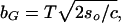
where ≡ ∂F̄/∂N_e = −f + zσN. The situation is shown in Fig. 1. Here −iN_e plays the role of time, F plays the role of position, ℏ = 1, and mass m = 1/cb².

Fig 1.

Nucleation free-energy profiles in trap escape, as a function of the number of escaped residues N_e. Shown are the mean free-energy profile (dashed line) and a typical profile for sequences constrained to have barriers smaller than E+F^≠−(F(b, T)−F^≠). Also shown schematically is the propagator G(F, N_e) for various values of N_e. The system rapidly relaxes to ground-state wavefunction after 𝒪(1) steps (see Appendix).

The free propagator G_F(F(b, T), N|E, 0) is straightforward:

where F̄(N_e) is again the typical free energy profile in Eq. 5.

We have been unable to obtain an exact, closed-form solution for the nonseparable, time-dependent problem with boundaries. However, we give in Appendix several analytical solutions in some reasonable limiting cases and solve the problem numerically in general.

There are polynomially many nucleation sites for a contiguous nucleus, which can be estimated geometrically. We equate this with the number of possible ways or routes N_R to escape from a trap. If any of these nucleation sites are buffed to F^≠, the trap then is assumed to be buffed to F^≠. We assume independent buffing probabilities for each of the distinct routes. Then the probability that n of the routes are buffed is simply a binomial distribution for n events, the probability of each of which is φ(F^≠), given in Eq. 8. Then the probability that at least one route is buffed to F^≠, i.e. the probability that a given trap of energy E is buffed, is p_B(F^≠|E, b) = 1 − (1 − φ(F^≠))^N_R.

Density of States and Density of Traps

To determine whether a sequence, rather than just a specific trap, is buffed we need to know how many candidate traps have energy E. We estimate the number of candidate traps using the mean-field calculation for a “typical” sequence. Then the effects of fluctuations sequence to sequence can be investigated.

A configurational state is a local trap if all states kinetically connected to it by a single local move are higher in energy. Because the number of states connected to a given state equals Nν when each residue can move to ν other states on average, there is a polynomial fraction of traps on uncorrelated landscapes (17), f_T ≈ 1/Nν. On a correlated landscape, however, there is an exponentially small fraction of traps. To see this, let the conditional probability that a state has energy E′ given that it shares a fraction of q contacts with a state of energy E be P_q(E′|E). Then the fraction of states at energy E that are traps is given by the expression f_T(E) = (∫ dE′ P_q(E′|E))^Nν, with q suitably chosen as described below.

For a Hamiltonian consisting of interacting sets of p contacts, the conditional probability P_q(E′|E) obeys a Gaussian distribution centered on q^pE with variance 2B²(1 − q^2p) (18). Thus when q → 1, P_q(E′|E) → δ(E′ − E), and when q → 0 or p → ∞, the states become uncorrelated and P_q(E′|E) → P(E′). When p = 1, the landscape statistics of a two-body Hamiltonian are recovered. The more “many-body” the Hamiltonian is, the more decorrelated states of a given structural similarity are.

Because we are looking at states connected by single kinetic moves, we take E′ = E + δE and q = 1 − δq, with δE ∼ 𝒪(N) but small compared to E, and δq ∼ 𝒪(N⁻¹), because we envision local moves of an intensive number of residues. Then the distribution of δE becomes a Gaussian with mean pEδq and variance 4B²pδq, and the fraction of traps becomes f_T(E) = [(1/2)erfc(E/2B)]^Nν where erfc(x) is the complementary error function. Thus f_T is of the form of a fraction raised to a large power. It is not significant until the argument or erfc (which is intensive) is fairly large and negative. Then the error function may be asymptotically expanded around one to yield

where c(E) = ν(πpδqE²/B²)^−1/2exp(−pδqE²/2B²) is a function of an intensive argument. Retracing the steps in the above argument for an uncorrelated landscape (or letting p → ∞) results in nearly every state constituting a trap, consistent with previous results.

The total number of traps Ω_T(E, b) at energy E is then the total number of states Ω times the fraction P(E) of those states at energy E, times the fraction f_T(E) of those states that are traps. A plot of the log number of states and log number of traps is shown in Fig. 2.

Fig 2.

Long-dashed line, log number of states vs. energy; solid line, approximate log number of traps from Eq. 11; short-dashed line, log number of traps for the error function expression of f_T in the text above Eq. 11. The approximation is accurate for energies near the ground state but falls off too rapidly for energies near 0. There are still traps at E=0, because states may have positive energies as well. Estimates are used here for the number of states per residue (Ω = e^N×2), system size (N=100), and number of connected states (ν =1). Pair interactions are taken (p=1), energies are in units of B, and δq =1/N.

The probability that all the traps at energy E will be buffed to F^≠ is

assuming independent buffing probabilities for each trap. This assumption is likely to underestimate P_B. On the other hand we have assumed independent probabilities for each of the N_R routes out of a given trap to be buffed. This overestimates the value of p_B, bringing it closer to unity.

As energy increases above that of the ground state, the quantity P_B rapidly approaches a value of unity. It is hardest to buff out the lowest energies even considering that there are more traps at higher energies that must be buffed out. The fraction of sequences with available traps buffed at all energies that may be thermally occupied is

Sequences with Buffed Landscapes

Let the system have nonextensive gap Δ and be rugged enough so that the ground state is thermodynamically stable at the temperature of the earth, b > b_G in Eq. 6 (Fig. 3 shows a schematic of buffing between low-energy states). Note that all the thermodynamic properties of buffed landscapes are still the same as for random sequences. For example, configurational states still have variances in energies, thus there is little or no thermal entropy left in the system when b > b_G. It is the kinetic properties of the system that are different. Because the ground state is competing with polynomially other low-energy states, its Boltzmann weight is given by w_N ≈ (1 + c′N^γe^−Δ/T)⁻¹, where c′ is a constant of 𝒪(1), and γ is an <1. Thus, even for a nonextensive gap Δ ∼ 𝒪(N^1/2), the system will still have large Boltzmann weight in the ground state.

Fig 3.

Schematic of the energy landscape for a sequence with buffed ground states, projected onto a configurational coordinate. The barriers between the ground states are reduced to F^≠, but the overall variance of energy between states is not reduced. The lowest kinetic barriers between the states determines the escape rate. Along the coordinate(s) where the landscape is buffed, the kinetic barriers between states are reduced.

How rare are these buffed sequences as system size grows larger? Using Eq. 8 and the results from Appendix, we find an asymptotic expression for the fraction of surviving paths. To leading order,

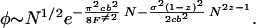The prefactor arises from the free propagator. In the exponent, the first term is a diffusion term that corresponds physically to the fact that buffed sequences are rare because of the likelihood of the specific free-energy profile to fluctuate outside of ±F^≠ after N steps. The second term in the exponent comes from the forcing term in the diffusion equation and embodies the fact that buffed sequences are rare because typical sequences follow the average free-energy profile. However, perhaps unexpectedly, the forcing term is subdominant, scaling more weakly with N (recall z is between 1/2 and 2/3, because the nucleus is roughened). Because φ is exponentially small, the probability that a trap is buffed over any route [in the expression for p_B(F^≠|E, b) above] has only polynomial corrections: p_B ≃ Nφ.

Because it is hardest to buff out the lowest energies, a sequence can be said to be buffed when a band of energies starting at the ground state and scaling polynomially with system size have all traps buffed to F^≠. Buffing out polynomially many competing ground states gives (from Eq. 13) P_B ≈ p_Be^aNα with α < 1. This again modifies the scaling by only subdominant corrections. From Eq. 14, more rugged sequences are harder to buff. The fraction of buffed sequences stable in their ground state at biological temperatures thus is dominated by those sequences having b² = b in Eq. 6. The fraction of sequences P_R having this ruggedness is given through Eq. 3. The total fraction of buffed sequences P_BUFF is then given by P_R(b_G)P_B(F^≠, b_G) or

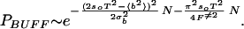For numerical values of the pair-interaction energies, such as those in the Miyazawa–Jernigan matrix, and naturally occurring amino acid abundances, sequence-to-sequence fluctuations of the barrier (second term in the exponent in Eq. 15) dominate the possibility of finding a buffed foldable sequence, with the probability of finding a sufficiently rugged composition playing a secondary role.

From Eqs. 4 and 15 we see that the relative rareness of buffed vs. funneled sequences becomes a quantitative issue, i.e. for a gap Δ to be thermodynamically relevant on a funneled landscape, Δ ∼ O(N). We address this in Fig. 4, where the fraction of sequences buffed to F^≠ = 4k_BT is plotted as a function of chain length N as well as the fraction of sequences sufficiently gapped so that the forward folding barrier is 4k_BT. The folding barrier is determined from a capillarity model; however, the gap still must scale extensively with chain length to ensure a constant ratio of T_F/T_G. There is a crossover in the figure beyond which it becomes easier to funnel. However, for short sequences as well as for longer sequences with degrees of freedom removed (due, for example, to native secondary or tertiary structure formation), buffing becomes more likely.

Fig 4.

The fraction of foldable sequences, on a log scale, as a function of chain length N. Both funneling and buffing mechanisms are shown here. Dashed line, fraction of funneled sequences with forward folding barrier F^≠=4k_BT, and T_F/T_G = 1.6; solid line, fraction of sequences buffed to F^≠=4k_BT. The adiabatic approximation for the Green's function in Eq. 9 is used (see Appendix). The crossover from buffing to funneling suggests the possibility of a compound mechanism for generating a functional protein sequence. The funneling mechanism removes most of the entropy while guiding the protein to a smaller ensemble of similar structures. Then for this reduced collection of states, dynamics between individual traps is most likely mediated by buffing. This dynamics may be related to functionally important motions in proteins (1). For funneled sequences we assume that no ruggedness selection occurs. We scale the Miyazawa–Jernigan interaction parameters so that in our units T_F/T_G ≈ 1.6, a common value taken from the literature (19). Buffed sequences must be selected to be sufficiently rugged to be stable at biological temperatures and must have low kinetic barriers to be accessible on biological time scales. (Inset) Comparison of the fraction of buffed sequences from the adiabatic approximation and from full numerical solution to Eq. 9. Several values of ruggedness are plotted. Circle, b=1.255; triangle, b=1.4; square, b=2.0.

Discussion

With increasing chain length it becomes exponentially rare for sequences to be significantly buffed. Likewise it is exponentially difficult to be funneled, thus the question is: Which exponential wins? Our estimates suggest that funneling overall is the dominant mechanism at least for larger proteins that fold on biological time scales. Still, the buffing mechanism raises some interesting practical questions.

Is it possible to design and synthesize a “buffed foldable protein?” Despite their rareness, buffed proteins probably exist and would be interesting objects, because they would possess a polynomial number of accessible states that could act as memories. Unfortunately, unlike funneled landscapes, the definition of buffed landscapes does not immediately lead to a design algorithm. We note that only recently has the funneling recipe been explicitly used in achieving foldability de novo in the laboratory (W. Jin, O. Kambara, H. Sasakawa, A. Tamura, and S. Takada, private communication). Still, combinatorial strategies are possible. Although natural protein landscapes are most likely funneled, the buffing mechanism may play a partial role in folding kinetics. Once a significant part of the protein is at least locally fixed by the funneling mechanism, the entropy is reduced to a level at which buffing can occur. This can act to remove specific intermediates or high-energy transition states on the landscape.

Other mechanisms in the spirit of buffing may exist that can facilitate folding. One can envision “antibuffed” or “gated” landscapes that have regions of phase space closed off by high-energy barriers, such that the system folds faster by exploring a smaller region of phase space, and avoiding regions that may contain deep traps. The fraction of sequences having gated landscapes may be worked out in a similar fashion as the fraction of buffed landscapes. Such a corralling mechanism on a funneled landscape is one way of describing the gatekeeper residues discovered by Otzen and Oliveberg in protein S6 (20). Gating is similar in spirit to Levinthal's (21) original resolution to the kinetic paradoxes in protein folding as well as issues that arise when considering kinetic partitioning mechanisms (22). Gating may also play a role in avoiding misfolded protein structures responsible for aggregation-related diseases.

Funneling is a sufficient and likely but not necessary condition for achieving foldability. However, the above folding mechanisms are not mutually exclusive: Funneled proteins may also exhibit buffing. The extent to which buffing occurs in real proteins may be tested, for example, by looking at the mutational sensitivity of the weights of nonnative transient folding intermediates. Two candidates for these studies are the α-helical early-folding intermediate in β-lactalbumin (23) and the major kinetic traps in α-lactalbumin, the populations of which may be measured by disulfide scrambling (24).

The ways evolution has assisted the folding and function of proteins are manifold: We have described an alternative to funneling here. It will be interesting to see what other organizing principles of energy landscapes are important in describing structural and functional biology.

Solutions for Green's Function for Buffing

In this section we find approximate solutions to Eq. 9 to derive analytical expressions for φ(F^≠) in Eq. 8. We are interested here in finding the fraction of sequences with kinetic barriers that are below F^≠, where F^≠ ∼ 𝒪(k_BT). The wave-packet solution to Eq. 9 spreads out diffusively to width F^≠ in a number of steps N*_e ∼ F^≠2/b². But because both F^≠ and b are ∼𝒪(k_BT), N*_e ∼ 𝒪(1). Hence we expect that by N steps the wave function will have long since relaxed to the ground state. This also means that the time rate of change of the drift term in Eq. 9 is slow compared to the rate at which the wave packet relaxes. The adiabatic parameter is given here by |〈2|∂H/∂N_e|1〉/(E₂ − E₁)²|, where the numerator is the matrix element of (N_e) (∂G/∂F) between the ground and first excited eigenfunctions of the unperturbed Hamiltonian, and the denominator is the difference in the first excited and ground-state eigenvalues. A straightforward calculation gives the parameter as L³σ/π⁴b⁴N (where L ≡ F is given above Eq. 8 and is of order of a few k_BT). This parameter is much smaller than unity over the whole range of N_e for all energies contributing to barriers to be buffed. Hence we conclude that here the adiabatic approximation is a good one. Then the time-dependent prefactor (N_e) in Eq. 9 then may be treated as a constant parameter and the solution then given in terms of that parameter.

The adiabatic approximation is a special case of a more general transformation. We may eliminate the drift term in Eq. 9 by letting G(F, N_e) = K(F, N_e)exp(g(F, N_e)), with g(F, N_e) = (N_e)F/(cb²) − (1/2cb²)∫ dN′_e(N′_e)². This yields a new differential equation for K(F, N_e) with a time- and position-dependent sink term:

Because in the adiabatic approximation the coefficient of the drift term could be treated as a constant, the first term in the parentheses in Eq. 16 (∝(N_e)) can be neglected, because it is the time derivative of the drift coefficient. Then for N_e> 0, K(F, N_e) satisfies a simple diffusion equation with absorbing walls such that K(F(b, T) − F^≠, N_e) = K(E + F^≠, N_e) = 0, and the initial condition is K(F, N_e) = δ(F − E). Thus the expansion in eigenfunctions may readily be written down. As we mentioned above, ground-state dominance is an excellent approximation for N_e > 1, thus the solution is then given by the ground-state term in the eigenfunction expansion,

where δF^≠ ≡ F^≠ − F(b, T). The propagator to (F(b, T), N) is then G(F(b, T), N). The fraction of surviving paths is then given by φ(F^≠) in Eq. 8 along with Eq. 17 and the free propagator in Eq. 10.

The N scaling of the fraction of buffed sequences may be checked with an exactly solvable model. For near ground states buffed to F^≠, the width L = 2F^≠ does not scale with N, and thus can be replaced by a parabolic potential of a fixed, effective width. Then V(F(N_e)|F^≠) in Eq. 16 is replaced by ½ω²F²/cb², where the effective frequency ω determines the spring stiffness. Here the differential Eq. 16 is equivalent to a Schrodinger equation with ℏ = 1, time t replaced by −iN_e, position replaced by free energy F, and particle mass replaced by 1/cb². Shifting coordinates so the effective harmonic well is centered at 0, the solution to Eq. 16 may be obtained exactly by integrating the Lagrangian over all paths (25). The result is

where in the quantum-mechanical analogy S_CL represents the (extremal) action along the classical path. Calculating this for large N shows that, analogous to the “forcing term” we saw before, the classical action S_CL(F, N|F_o, 0) does not dominate the scaling behavior. Instead the prefactor, measuring deviations from the path of least action, plays the most important role, scaling as ∼e^−ωN/2 for large N. Following the same arguments as before, this is essentially the scaling law for the fraction of buffed sequences. Comparing the scaling law here with that in Eq. 15, we see that the effective frequency ω is such that the unforced propagators in the hard-wall and parabolic-wall cases have the same survival probability after N steps.

References

- 1.Frauenfelder H., Sligar, S. G. & Wolynes, P. G. (1991) Science 254, 1598-1603. [DOI] [PubMed] [Google Scholar]
- 2.Leopold P. E., Montal, M. & Onuchic, J. N. (1992) Proc. Natl. Acad. Sci. USA 89, 8721-8725. [DOI] [PMC free article] [PubMed] [Google Scholar]
- 3.Bryngelson J. D. & Wolynes, P. G. (1987) Proc. Natl. Acad. Sci. USA 84, 7524-7528. [DOI] [PMC free article] [PubMed] [Google Scholar]
- 4.Ueda Y., Taketomi, H. & Gō, N. (1975) Int. J. Peptide Protein Res. 7, 445-459. [PubMed] [Google Scholar]
- 5.Onuchic J. N., Socci, N. D., Luthey-Schulten, Z. & Wolynes, P. G. (1996) Fold. Des. 1, 441-450. [DOI] [PubMed] [Google Scholar]
- 6.Clementi C., Jennings, P. A. & Onuchic, J. N. (2000) Proc. Natl. Acad. Sci. USA 97, 5871-5876. [DOI] [PMC free article] [PubMed] [Google Scholar]
- 7.Takada S. (1999) Proc. Natl. Acad. Sci. USA 96, 11698-11700. [DOI] [PMC free article] [PubMed] [Google Scholar]
- 8.Govindarajan S. & Goldstein, R. A. (1997) Proteins Struct. Funct. Genet. 29, 461-466. [DOI] [PubMed] [Google Scholar]
- 9.Villain J. (1985) J. Phys. 46, 1843-1852. [Google Scholar]
- 10.Kirkpatrick T. R., Thirumalai, D. & Wolynes, P. G. (1989) Phys. Rev. A 40, 1045-1054. [DOI] [PubMed] [Google Scholar]
- 11.Pande V. S., Grosberg, A. Y. & Tanaka, T. (1997) Biophys. J. 73, 3192-3210. [DOI] [PMC free article] [PubMed] [Google Scholar]
- 12.Miyazawa S. & Jernigan, R. L. (1996) J. Mol. Biol. 256, 623-644. [DOI] [PubMed] [Google Scholar]
- 13.Derrida B. (1981) Phys. Rev. B 24, 2613-2626. [Google Scholar]
- 14.S̆ali A., Shakhnovich, E. & Karplus, M. (1994) J. Mol. Biol. 235, 1614-1636. [DOI] [PubMed] [Google Scholar]
- 15.Wolynes P. G. (1997) Proc. Natl. Acad. Sci. USA 94, 6170-6175. [DOI] [PMC free article] [PubMed] [Google Scholar]
- 16.Wang J., Plotkin, S. S. & Wolynes, P. G. (1997) J. Phys. I [French] 7, 395-421. [Google Scholar]
- 17.Bryngelson J. D. & Wolynes, P. G. (1989) J. Phys. Chem. 93, 6902-6915. [Google Scholar]
- 18.Plotkin S. S. & Onuchic, J. N. (2002) Q. Rev. Biophys. 35, 205-286. [DOI] [PubMed] [Google Scholar]
- 19.Onuchic J. N., Wolynes, P. G., Luthey-Schulten, Z. & Socci, N. D. (1995) Proc. Natl. Acad. Sci. USA 92, 3626-3630. [DOI] [PMC free article] [PubMed] [Google Scholar]
- 20.Otzen D. E. & Oliveberg, M. (1999) Proc. Natl. Acad. Sci. USA 96, 11746-11751. [DOI] [PMC free article] [PubMed] [Google Scholar]
- 21.Levinthal C. (1969) in Mossbauer Spectroscopy in Biological Systems, eds. DeBrunner, P., Tsibris, J. & Munck, E. (Univ. of Illinois Press, Urbana), pp. 22–24.
- 22.Thirumalai D. (1995) J. Phys. I [French] 5, 1457-1467. [Google Scholar]
- 23.Kuwata K., Shastry, R., Cheng, H., Hoshino, M., Batt, C. A., Goto, Y. & Roder, H. (2001) Nat. Struct. Biol. 8, 151-155. [DOI] [PubMed] [Google Scholar]
- 24.Chang J.-Y. (2002) J. Biol. Chem. 277, 120-126. [DOI] [PubMed] [Google Scholar]
- 25.Feynman R. P. & Hibbs, A. R., (1965) Quantum Mechanics and Path Integrals (McGraw–Hill, New York).