Statistical Validation of Image Segmentation Quality Based on a Spatial Overlap Index

Abstract

Rationale and Objectives

To examine a statistical validation method based on the spatial overlap between two sets of segmentations of the same anatomy.

Materials and Methods

The Dice similarity coefficient (DSC) was used as a statistical validation metric to evaluate the performance of both the reproducibility of manual segmentations and the spatial overlap accuracy of automated probabilistic fractional segmentation of MR images, illustrated on two clinical examples. Example 1: 10 consecutive cases of prostate brachytherapy patients underwent both preoperative 1.5T and intraoperative 0.5T MR imaging. For each case, 5 repeated manual segmentations of the prostate peripheral zone were performed separately on preoperative and on intraoperative images. Example 2: A semi-automated probabilistic fractional segmentation algorithm was applied to MR imaging of 9 cases with 3 types of brain tumors. DSC values were computed and logit-transformed values were compared in the mean with the analysis of variance (ANOVA).

Results

Example 1: The mean DSCs of 0.883 (range, 0.876–0.893) with 1.5T preoperative MRI and 0.838 (range, 0.819–0.852) with 0.5T intraoperative MRI (P < .001) were within and at the margin of the range of good reproducibility, respectively. Example 2: Wide ranges of DSC were observed in brain tumor segmentations: Meningiomas (0.519–0.893), astrocytomas (0.487–0.972), and other mixed gliomas (0.490–0.899).

Conclusion

The DSC value is a simple and useful summary measure of spatial overlap, which can be applied to studies of reproducibility and accuracy in image segmentation. We observed generally satisfactory but variable validation results in two clinical applications. This metric may be adapted for similar validation tasks.

Magnetic resonance imaging (MRI) provides indispensable information about anatomy and pathology, enabling quantitative pathologic and clinical evaluations. Segmentation is an important image-processing step by which regions of an image are classified according to the presence of relevant anatomic features. For example, segmentation of MRI of the brain assigns a unique label (eg, white matter, gray matter, lesions, cerebrospinal fluid, to each voxel in an input gray-scale image) (1). Segmentation methods typically yield binary or categoric classification results. However, continuous classification schemes (eg, volume size, distance between the volume surfaces, percentage of overlap voxels, percentage of highly discrepant voxels, and probability-based fractional segmentation) are increasingly becoming commonplace (2,3). The performance of segmentation methods has a direct impact on the detection and target definition, as well as monitoring of disease progression. Thus, the main clinical goal of surgical planning and quantitative monitoring of disease progression requires segmentation methods with high reproducibility because of the limited number of images available per patient.

Several recent articles have addressed the importance of developing new automated segmentation methods in addition to binary classification, using overlap mixture intensity distributions of abnormal and normal tissues (4–6), as well as a probabilistic fractional segmentation methods on a continuous probability scale per voxel (2,3). These methods used geometric and probabilistic models to allow improved tissue volume estimates and contrast among tissue types (7–10). An overview and comparison of several existing algorithms for brain segmentation (eg, finite normal mixture histograms, genetic algorithms, and hidden Markov random field methods using percent correct identified voxels against digital phantoms) are found in the literature (7).

However, it is a challenging task to evaluate the accuracy and reproducibility of MRI segmentations. To conduct a validation analysis of the quality of image segmentation, it is typically necessary to know a voxel-wise gold standard. Under a simple binary truth (here labeled, T), this gold standard is defined as an indicator of true tissue class per voxel, ie, the target class (C₁) such as malignant tumor, and the background class (C₀) such as the remaining healthy tissues. Unfortunately, it is often impractical to know T only based on clinical data.

Various alternative methods have been sought to carry out statistical validations. A useful method is to construct phantoms, either physically or digitally, with known T, specified before building such a phantom. Because it is difficult to construct a physical phantom that can mimic the tissue properties of the human body, great efforts have been devoted to building digital phantoms that are both realistic and assessable by the radiologic community. Simulated MR digital brain phantom images of a normal subject or one with multiple sclerosis may be downloaded online from the Montreal BrainWeb (http://www.bic.mni.mcgill.ca/brainweb) (11,12). Nevertheless, even sophisticated phantoms may not yield clinical images with full range of characteristics frequently observed in practice, such as partial volume artifacts, intensity heterogeneity, noise, and normal and pathologic anatomic variability.

Without a known gold standard obtained by non-imaging methods such as histology, the validation task becomes an assessment of reliability or reproducibility of segmentation. A simple spatial overlap index is the Dice similarity coefficient (DSC), first proposed by Dice (13). Dice similarity coefficient is a spatial overlap index and a reproducibility validation metric. It was also called the proportion of specific agreement by Fleiss (14). The value of a DSC ranges from 0, indicating no spatial overlap between two sets of binary segmentation results, to 1, indicating complete overlap. Dice similarity coefficient has been adopted to validate the segmentation of white matter lesions in MRIs (15) and the peripheral zone (PZ) of the prostate gland in prostate brachytherapy (16). Other validation metrics considered for statistical validation included Jaccard similarity coefficient (17), odds ratio (18), receiver operating characteristic analysis (19–22), mutual information (3,22), and distance-based statistics (23,24).

In the present work, we applied and extended the DSC metric on two clinical examples analyzed previously. We aimed to validate (A) repeated binary segmentation of preoperative 1.5T and intraoperative 0.5T MRIs of the prostate’s PZ collected before and during brachytherapy for prostate cancer (16); and (B) semi-automated probabilistic fractional segmentation of MRIs of three different types of brain tumors, against a composite voxel-wise gold standard derived from repeated expert manual segmentations of the images (25). For both the prostate and brain datasets, segmentations were performed and reported previously (16,25). Here we have extended our methodology and shown a statistical validation analysis using these existing databases.

MATERIALS AND METHODS

Example 1: Magnetic Resonance Imaging of the Prostate Peripheral Zone

Imaging protocol

A total of 10 sequential MR-guided brachytherapy cases were identified retrospectively from clinical practice. We excluded the cases who had received any brachytreatment or previous external beam radiation therapy, which could confound shape and MR signal intensity changes in the gland (16). Both preoperative and intraoperative imaging was performed as follows:

1. Preoperative Imaging: All patients underwent preoperative 1.5T MR imaging using an endorectal coil (MedRad, Indianola, PA) with an integrated pelvic-phased multicoil array (Signa LX; GE Medical Systems, Milwaukee, WI). The endorectal coil is a receive-only coil mounted inside a latex balloon, and assumed a diameter of 4–6 cm, once inflated in the patient’s rectum. The patient was placed in a supine position in the closed-bore magnet for the imaging examination. The axial T2-weighted images were fast spin echo images (4,050/135; field of view, 12 cm; section thickness, 3 mm; section gap, 0 mm; matrix, 256 × 256; 3 signal averages). Typical acquisition times were 5–6 minutes.

2. Intraoperative Imaging: Imaging was performed in the open-configuration 0.5T MR scanner (Signa SP; General Electric Medical Systems). Each patient was placed in the lithotomy position to facilitate prostate brachytherapy via a perineal template. The perineal template was fixed in place by a rectal obturator (2 cm in diameter). T2-weighted fast spin echo images (axial and coronal, 6,400/100; field of view, 24 cm; section thickness, 5 mm; section gap, 0 mm; matrix, 256 × 256; 2 signal averages) were acquired in the MR scanner using a flexible external pelvic wraparound coil, with typical acquisition times of 6 minutes.

Repeated manual segmentations

The three-dimensional Slicer (http://www.slicer.org) (26) was used as a surgical simulation and navigation tool and to facilitate manual segmentation. Manual contouring of two areas of the prostate, the PZ, and the central gland, was performed by two segmenters using the T2-weighted images from the 1.5T and 0.5T studies. Each segmenter independently and blindly outlined the PZ in five of these randomly selected 10 cases. The manual segmentations of the same preoperative 1.5T and intraoperative 0.5T image were repeated five times. When segmenting the intraoperative 0.5T images, the segmenters were allowed to examine preoperative 1.5T images, as is done in clinical practice.

Example 2: Magnetic Resonance Imaging of Brain Tumors

Imaging protocol

A total of nine patients were selected randomly for the purpose of validation from a neurosurgical database of 260 brain tumor patients, of which three cases had meningiomas, three cases had astrocytomas, and three remaining cases had other mixed low-grade gliomas (G) (25). The imaging protocol consisted of the following parameters: patient heads were imaged in the sagittal planes with a 1.5T MR imaging system (Signa, GE Medical Systems), with a postcontrast 3-dimensional sagittal spoiled gradient recalled acquisition with contiguous slices (flip angle, 45°); repetition time of 35 ms; echo time of 7 ms; field of view of 240 mm; slice-thickness of 1.5 mm; 256 × 256 × 124 matrix.

Manual segmentation

Using a randomly selected single 2-dimensional slice containing the tumor from MR imaging, an interactive segmentation tool (MRX; GE Medical Systems, Schenectady, NY) was used. Three segmenters, blinded to the semi-automated probabilistic fractional segmentation results, independently outlined the target tumors. They extracted the tumor boundary as perceived on spoiled gradient recalled acquisition. An anatomic object was defined by a closed contour, and the computer program labeled every voxel of the enclosed volume.

Probabilistic fractional segmentation

An automated probabilistic fractional segmentation algorithm was applied (2,3), which yielded voxel-wise continuous probabilistic measures in the range of [0,1], indicative of the likelihood of the brain tumor class. To derive such probabilities, the relative signal intensity was modeled as a normal mixture of the two classes based on an initial semiautomated binary segmentation.

Dice Similarity Coefficient and Logit Transformation

The main validation metric of spatial overlap index was DSC (13). The DSC measures the spatial overlap between two segmentations, A and B target regions, and is defined as DSC(A,B)= 2(A∩B)/(A+B) where ∩ is the intersection (Fig 1). In binary manual segmentation, this coefficient may be derived from a two-by-two contingency table of segmentation classification probabilities (Table 1). Conceptually that DSC is also a special case of the kappa statistic commonly used in reliability analysis, when there is a much larger number of background voxels than that of the target voxels, as shown previously by Zijdenbos et al (15).

Figure 1.

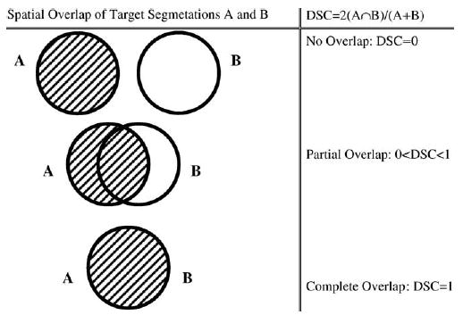
The Dice similarity coefficient representing spatial overlap and reproducibility, where DSC = 2 (intersected region)/(sum of region A and region B).

Table 1.

Two-by-Two Contingency Table of Four Possible Probabilities of Segmentation Results Based on an Image, Along with the Definition of Disc Similarity Coefficient and the Logit Transformed Dice Similarity Coefficient, Where the Target is the Object (eg, the Prostate Peripheral Zone in Example 1 and the Brain Tumor in Example 2) to be Segmented

		Segmentation 2	(S2)
Segmentation	Pair	D2 = 0 (Background)	D2 = 1 (Target)	Marginal Total
Segmentation 1	D1 = 0 (Background)	P00	p01	p0·
(S1)	D1 = 1 (Target)	P10	p11	p1·
Marginal total		P·0	P·1	1

Note. $\begin{array}{l}DSC(S_1,S_2)=\frac{2P\{(D_1=1)\mathrm{\hspace{0.17em} }\cap \mathrm{\hspace{0.17em} }(D_2=1)\}}{P(D_1=1)+P(D_2=1)}=\frac{2p_{11}}{P_{\cdot 1}{p}_{1\cdot }}=\text{in\hspace{0.28em}}[0,1],\text{and}\\ logit\{DSC(S_1,S_2)\}=\text{ln}\left\{\frac{DSC(S_1,S_2)}{1-DSC(S_1,S_2)}\right\}\text{in}(-\infty ,\infty ).\end{array}$

Furthermore, because DSC has a restricted range of [0,1] and is often close to the value of 1, we have found it useful to adopt a logit transformation for the purpose of statistical inferences, where logit(DSC)=ln{DSC/(1−DSC)}. This monotone transformation maps the domain of [0,1] to the unbounded range (−∞,∞), and logit(0.5) = 0. Agresti (18) showed that for large sample size (in our case, the number of voxels), the distribution of the logit transformed proportions and rates followed a normal distribution, asymptotically with a large number of voxels. A statistical test of normality may be conducted by a z-test under a voxel-wise independence assumption (27). As recommended by Zijdenbos et al (15) in the literature of image validation an good overlap occurs when DSC >0.700, or equivalently, logit(DSC) >0.847. Based on the analysis of the kappa statistic, an excellent agreement occurs when k >0.75, as recommended by Fleiss (14). In the present work, we applied this important transformation to all DSC values before conducting any statistical comparisons and hypothesis testing.

Statistical Methods for Example 1: Magnetic Resonance Imaging of the Prostate Peripheral Zone

Summary statistics of DSC

In our clinical practice, the PZ of the prostate is the clinical target volume for brachytherapy. Therefore, in our secondary analysis, the main focus was placed on analyzing the reproducibility of PZ segmentations. Previously, we showed that preoperative 1.5T MRI provided better spatial resolution and contrast, compared with intraoperative 0.5T MRI (16). We thus developed a novel deformable registration method, used to align pretreatment 1.5T images with 0.5T intraoperative images to improve the information content of the latter.

In the current analysis, we compared the corresponding reproducibility results based on preoperative versus intraoperative images using all pair-wise spatial overlaps of five repeated segmentations of the PZs of the 10 brachytherapy cases pooled over the two image segmenters because we did not find significant differences between these segmenters. Moreover, we tested whether there existed a learning-curve effect over time.

We labeled a segmentation pair as S_k and S_k’ from all 10 parings of the five repeated segmentations, where (k,k’) = {(1,2); (2,3); (3, 4); (4, 5); (1,3); (2,4); (3,5); (1,4); (2,5); (1,5)}. (Note: The index of k indicated a natural sequence in time, ie, S₂ took place after S₁, S₃ took place after S₂, and so on.) Thus, when (k,k’) = {(1,2); (2,3); (3,4); (4,5)}, there was no session in between the segmentation pair. Similarly, we labeled (k,k’) = {(1,3); (2,4); (3,5)} with one session, (k,k’) = {(1,4); (2,5); (3,5)} with two sessions, (k,k’) = {(1,4); (2,5)} with three sessions, and finally (k,k’) = {(1,5)} with four sessions in between their corresponding segmentation pairs, respectively.

For each segmentation pair, summary statistics including the means and the standard deviations of DSC and logit(DSC) were computed over all 10 cases, separately for 1.5T and 0.5 images. In addition, boxplots of DSCs were created.

Analysis of variance

There were several clinical questions to be addressed using an analysis of variance (ANOVA) approach: (1) Was the reproducibility of the manual segmentations of PZ before and during brachytherapy satisfactory? (This was published elsewhere (16) and is essential knowledge for interventional planning and treatment.) (2) Was there a difference in reproducibility in segmenting preoperative 1.5T and intraoperative 0.5T images? (Note: The advantages of the reproducibility using preoperative 1.5T over intraoperative 0.5 images would justify the need for registering the 1.5T images onto 0.5 images using the deformable model developed earlier) (16). (3) Was there a learning curve affecting the segmenters over time? (4) Was there a case-to-case variation in segmentation quality of the PZs?

To answer the above questions, we constructed the following ANOVA model: Denote the variance components as M = preoperative 1.5T or intraoperative 0.5T MR, C = case, S = segmentation pair, and two possible interactions, S × M and S × C. Correspondingly, there were two imaging × 10 cases × 10 segmentation pairs =200 DSC values based on all pair-wise overlaps of the repeated segmentations. In our ANOVA model, the outcome variable was logit(DSC) with a normal error assumption. Thus, the model specification, written as the following regression equation, for logit-transformed DSC became:

$$\begin{array}{l}\text{logit}(\text{DSC})=\text{ln}\{\text{DSC}/(1-\text{DSC})\}\\ =\mu +\text{M}+\text{C}+\text{S}+\text{S}\times \text{M}+\text{S}\times \text{C}+\text{e},\end{array}$$ (1)

where normality was assumed for each component in the model; μ was the intercept and e is the residual error term. The F-test statistic and P value of each variance component were computed. Because here the reproducibility of segmentations was of main interest, the reduced ANOVA model in equation 1 did not include all other possible additional interaction terms, although the saturated model may also be considered.

In addition, we repeated a similar ANOVA to test the effect of segmentation by restricting the segmentation pairs only to those taking place sequentially and consecutively, ie, with S_k and S_k’ where (k,k’) = {(1,2); (2,3); (3,4); (4, 5)}.

Statistical Methods for Example 2: Magnetic Resonance Imaging of Brain Tumors

Estimation of a voxel-wise gold standard

The main purpose here was to evaluate the spatial overlap between the automated probabilistic fractional segmentation results against a composite voxel-wise gold standard, with the latter estimated based on three segmenters’ independent manual segmentation results. Our motivation here was that reasonably satisfactory and yet imperfect manual segmentations were observed from these three expert segmenters. Thus, the first step in our validation procedure was to estimate a binary gold standard by combining these multiple manual segmentations.

We applied our recently developed Simultaneous Truth and Performance Level Estimation (STAPLE) program (21,22,28), which is an automated expectation-maximization algorithm (29) for estimating the gold standard, along with the performance level of each segmentation repetition. For each voxel, a maximum likelihood estimate of the composite gold standard of tumor or background class was optimally determined over all image readers’ results (30). The details of this algorithm may be found in relevant work (21,22,28) and are omitted here.

Bi-beta modeling of mixture distributions

The manual segmentations were binary taking values of either 0 or 1, while the automated probabilistic fractional segmentation yielded a probabilistic interpretation, a continuous value in [0, 1], of the brain tumor class in each voxel. A convenient model for such probabilistic data was a mixture of two beta distributions, here called the bi-beta model (31). This model assumed that the distribution of the probabilistic fractional segmentation in the background class was F(x) ~ Beta(α₀β₀), while the distribution of the probabilistic fractional segmentation in the target brain tumor class was G(y) ~ Beta(α₁β₁), with different shape parameters of the two classes.

The estimates of the four beta shape parameters are obtained by matching the mean and variances of the beta distributions with what are found in each sample, separately for the background and the target voxels, as follows: from the sample data in gold standard class C₀, let the mean of the probabilistic data in the background class be $\overline{x}$ and the standard deviation be s_x; similarly, from the sample data in gold standard class C₁, let the mean and standard deviations be $\overline{y}$ and the standard deviation be s_y, respectively, then the estimates of the parameters in the bi-beta model are: ${\widehat{\alpha }}_0=\overline{x}\{\overline{x}(1-\overline{x})s_x^2-1\},{\widehat{\beta }}_0=(1-\overline{x})\{\overline{x}(1-\overline{x})s_x^2-1\}$; similarly, ${\widehat{\alpha }}_1=\overline{y}\{\overline{y}(1-\overline{y})s_y^2-1\}$, and ${\widehat{\beta }}_1=(1-\overline{y})\{\overline{y}(1-\overline{y})s_y^2-1\}$. Maximum likelihoods of the parameters may also be obtained instead of using the moment approach. However, the solutions are not explicit. Because a large number of voxels are available, the efficiency of the method of moments is reasonable.

The beta mixture model is flexible in parametric modeling probabilistic data and fractions (31). The parameters in this bi-beta model were estimated by matching the first two moments, ie, the mean and the standard deviation, of the distributions.

Dice similarity coefficient based on a probabilistic fractional segmentation

Because the probabilistic fractional segmentation yielded a continuous outcome in [0,1], at each arbitrary decision threshold, γ, the segmentation result was first discretized into a dichotomy. For simplicity, assume spatial independence for all individual voxels in classes C₀ and C₁. Label the measurements of C₀ as X_i (I = 1,…,m individuals or voxels), and the measurements of C₁ as Y_j (j = 1,…,n individuals or voxels). The corresponding gold standard variable is labeled as T for all of the (m + n) voxels in an image or a region of interest.

Without a loss of generality, further assume that a large threshold, γ, indicates an increased likelihood of a target class in each voxel. At each possible threshold γ, the underlying cumulative distributional function (c.d.f.) under class C₀ is F(γ). At the same threshold γ, the underlying c.d.f. under class C₁ is G(γ). Given γ, the true negative fraction (specificity, θ_γ0) and the true positive fraction (sensitivity, θ_γ1) respectively:

$${\theta }_{\gamma 0}=P(D\gamma =0|T=0)=P(X\le \gamma |T=0)=F(\gamma ),$$

and

$$\begin{array}{l}{\theta }_{\gamma 1}=P(D\gamma =1|T=1)=P(Y>\gamma |T=1)\\ =1-G(\gamma ).\end{array}$$ (2)

As demonstrated below, the spatial overlap measured by DSC_γ between the dichotomized segmentation result and the binary gold standard is a simple function of sensitivity (true-positive rate), specificity (true-negative rate), and the true fraction of the target voxels of the entire image. Assume that the target occupies the fraction of the entire image voxels with π = P(T). At any given decision threshold, γ, the probabilistic fractional segmentation data may be made binary. The DSC at the binarizing decision threshold against a binary gold standard may be expressed as a simple function of the sensitivity (θ_γ1), specificity (θ_γ0), and true target fraction (π) parameters. By Bayes’ theorem, it is given by:

$$\begin{array}{l}DS{C}_{\gamma }=\frac{2P\{(D_{\gamma }=1)\mathrm{\hspace{0.17em} }\cap \mathrm{\hspace{0.17em} }(T=1)\}}{P(D_{\gamma }=1)+P(T=1)}\\ =\frac{2P(D_{\gamma }=1|T=1)P(T=1)}{\begin{array}{l}\{P(D_{\gamma }=1|T=0)P(T=0)\\ +P(D_{\gamma }=1|T=1)P(T=1)\}+P(T=1)\end{array}}\\ =\frac{2{\theta }_{\gamma 1}\pi }{(1-{\theta }_{\gamma 0})(1-\pi )+(1+{\theta }_{\gamma 1})\pi }\\ =\frac{2{\theta }_{\gamma 1}\pi }{1-{\theta }_{\gamma 0}+({\theta }_{\gamma 0}+{\theta }_{\gamma 1})\pi }.\end{array}$$ (3)

Let γ have a uniform, Unif(0,1), prior distribution in [0,1]. The expected DSC over all range of γ∈[0,1] is $DSC={\int }_0^{1}DS{C}_{\gamma }d\gamma$, approximated via numerical integration.

As a possible future extension, a prior distribution h(γ) of the decision threshold γ may be assumed, and an expected DSC is given by $DSC={\int }_0^{1}DS{C}_{\gamma }h(\gamma )d\gamma$. The threshold was assumed to have a uniform distribution because of possible case-to-case variations. The justification for the integral over the threshold is an analog with receiver operating characteristic (ROC). However, more informative knowledge may be used to impose sharper prior distributions of this threshold. For example, if the threshold is known to be centered around 0.5, then a symmetric beta prior distribution with equal values of its two shape parameters may be assumed for γ. The expectation of DSC was calculated by a numerical integration over the range of all possible thresholds, γ∈[0,1]. The effect of the variability of the threshold may be evaluated, and an optimal operating threshold may be obtained by maximizing the corresponding DSC value.

Numerical Simulation of Dice Similarity Coefficients Under Bi-Beta Models

We used numerical integration to explore the relationship between several pre-specified bi-beta shape parameters and the corresponding DSC values. We considered several hypothetical scenarios for the mixture distributions with equal variances in the target and background classes. As the mean of a two-parameter Beta(α,β) distribution is α/(α+β) and the variance is αβ/{(α+β)²(α+β+1)} we set one of the two shape parameters of the distribution to 1 for simplicity. By varying the value of the other shape parameter, we achieved different underlying mixtures.

The beta shape parameters specified in each of the Monte-Carlo simulations with 500 random samples were: (α₀,β₀,α₁,β₁) = {(1,1,1,1,); (1,1.5,1.5,1);(1,3,3,1);(1,9,9,1)} in the bi-beta model. The total number of voxels was fixed to be 10,000, with π={10%; 15%} as the fraction of the target. The effects of the parameter and the target fraction on the resulting DSC were examined.

RESULTS

Example 1: Magnetic Resonance Imaging of the Prostate Peripheral Zone

Summary statistics of DSC

The preoperative and intraoperative images and intraoperative 0.5T T2-weighted MRIs of a case are shown in Figure 2. One of the five repeated manual segmentations results of the PZ on these images is given in the same figure. The boxplots of DSCs from preoperative 1.5T images and intraoperative 0.5T images by segmentation pair are presented in Figures 3 and 4, respectively.

Figure 2.

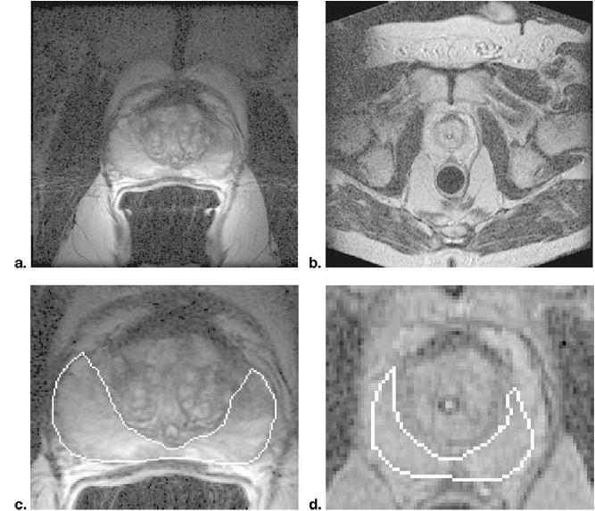
Prostate T2-weighted preoperative 1.5T MRI (a) and intraoperative 0.5T MRI (b) from the same brachytherapy patient, along with manual segmentations of the PZ on these 1.5T (c) and 0.5T (d) images, in detail. The DSC and reproducibility of PZ segmentations were significantly higher on the preoperative 1.5T image.

Figure 3.

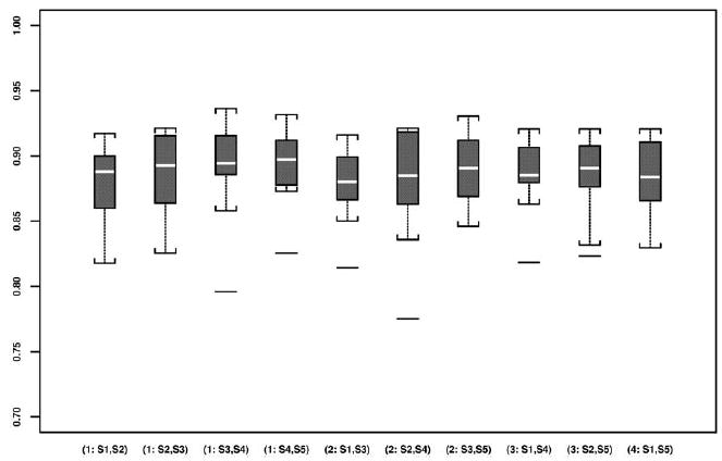
Boxplots of all DSCs based on all pair-wise repeated segmentations of the prostate PZ using preoperative 1.5T images.

Figure 4.

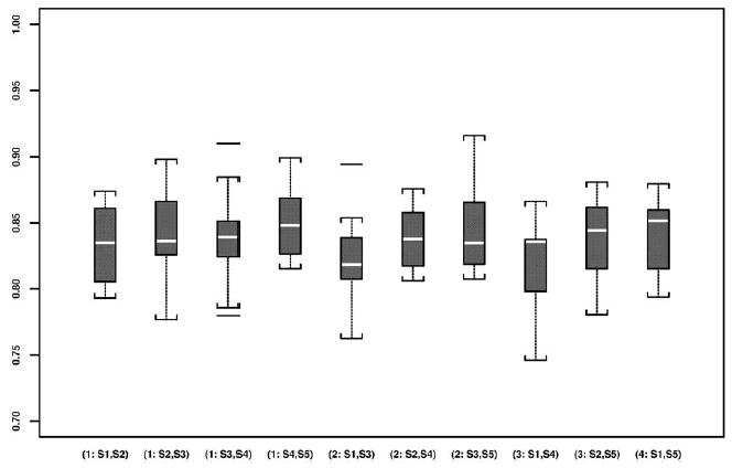
Boxplots of all DSCs based on all pair-wise repeated segmentations of the prostate PZ using intraoperative 0.5T images.

The means and standard deviations of the DSCs and logit(DSC) values of all segmentation pairs based on both preoperative 1.5T and intraoperative 0.5 images are given in Table 2. The preoperative and intraoperative imaging resulted in significantly higher reproducibility by mean logit (DSC) preoperatively than intraoperatively. The mean DSCs of the 10 cases were 0.883 (range, 0.876–0.893) preoperatively and 0.838 (range, 0.819–0.852) intraoperatively, with a statistical significant difference (P <.001).

Table 2.

Estimated Mean Pairwise Dice Similarity Coefficient and Logit Transformed Dice Similarity Coefficient Values in Five Repeated Segmentations of Each of the Ten Preoperative 1.5T Magnetic Resonance Images and Intraoperative 0.5T Magnetic Resonance Images of the Prostate Peripheral Zone

		DSC				Logit (DSC)
		1.5T	Pre Op	0.5T	Intra Op	1.5T	Pre Op	0.5T	Intra Op
No. of Sessions Between Segmentation Pair	Segmentation Pair	Mean	(SD)	Mean	(SD)	Mean	(SD)	Mean	(SD)
0	(S1, S2)	0.879	(0.031)	0.834	(0.030)	2.008	(0.279)	1.625	(0.216)
	(S2, S3)	0.887	(0.030)	0.841	(0.035)	2.090	(0.292)	1.686	(0.272)
	(S3, S4)	0.880	(0.039)	0.840	(0.039)	2.126	(0.369)	1.684	(0.312)
	(S4, S5)	0.893	(0.030)	0.852	(0.029)	2.159	(0.306)	1.770	(0.246)
1	(S1, S3)	0.878	(0.030)	0.823	(0.035)	2.003	(0.276)	1.559	(0.262)
	(S2, S4)	0.876	(0.045)	0.839	(0.024)	2.011	(0.388)	1.660	(0.181)
	(S3, S5)	0.888	(0.030)	0.847	(0.037)	2.108	(0.311)	1.742	(0.321)
2	(S1, S4)	0.885	(0.029)	0.819	(0.037)	2.070	(0.277)	1.525	(0.243)
	(S2, S5)	0.883	(0.033)	0.838	(0.030)	2.057	(0.301)	1.654	(0.217)
3	(S1, S5)	0.885	(0.029)	0.843	(0.028)	2.066	(0.280)	1.692	(0.203)

The normality assumptions were statistically verified by z-test after the logit transformation. Pair-wise logit-transformed of the 10 repeated segmentations of each of the 10 cases yielded nonsignificant normality test results, with all P values above .05 (range, .27–0.81 on 1.5T; .07–.80 on 0.5T). Comparing the mean logit(DSC) values, they were 2.070 (range, 2.011–2.159) on 1.5T versus 1.659 (range, 1.525–1.742) on 0.5T, thus, the segmentation reproducibility appeared higher based on preoperative images, and the P value was provided in the ANOVA results.

Analysis of variance

Tables 3 and 4 provide the two ANOVA results based on the variance component model for logit(DSC) values, as given in equation 1. According to all pair-wise DSCs over segmentation pairs (Table 3) and the DSCs of only sequentially consecutive segmentation pairs (Table 4), there was a statistically significant improvement in the reproducibility results using 1.5T over 0.5T images (P <.001). A case-to-case variation was also significant (P <.001).

Table 3.

The Analysis of Variance of All Pairwise Logit Transformed Dice Similarity Coefficient Values Based on Segmentations of Each of the Ten Preoperative 1.5T Magnetic Resonance Images and Intraoperative 0.5T Magnetic Resonance Images of the Prostate Peripheral Zone

Variance Component	Degree of Freedom	Sum of Squares	Mean Square	F-Test Statistic	P Value
MR (Pre vs Intra Op)	1	8.409	8.409	202.004	<.001
Case	9	9.478	1.053	25.299	<.001
Segmentation	9	0.611	0.068	1.631	.12
Segmentation × MR	9	0.143	0.016	0.381	.94
Segmentation × Case	81	1.108	0.014	0.329	>.99
Residuals	90	3.746	0.042	–	–

Note. MR; preoperative 1.5T, intraoperative 0.5T.

Table 4.

The Analysis of Variance of Only Sequentially Consecutive Logit Transformed Dice Similarity Coefficient Values Based on Segmentations of Each of the Ten Preoperative 1.5T Magnetic Resonance Images and Intraoperative 0.5T Magnetic Resonance Images of the Prostate Peripheral Zone

Variance Component	Degree of Freedom	Sum of Squares	Mean Square	F-Test Statistic	P Value
MR (Pre vs Intra Op)	1	3.272	3.272	66.797	<.001
Case	3	2.995	0.998	20.381	<.001
Segmentation	3	0.143	0.048	0.972	.41
Segmentation × MR	3	0.011	0.004	0.075	.97
Segmentation × Case	9	0.184	0.020	0.417	.92
Residuals	60	2.939	0.049	–	–

Note. MR; preoperative 1.5T, intraoperative 0.5T.

We did not observe a significant effect of segmentations among all pairs (P = .12; Table 3), nor was there a learning curve phenomenon (P = .97; Table 4). The two interaction terms included in equation 1 were not statistically significant either (Tables 3 and 4).

Example 2: Magnetic Resonance Imaging of Brain Tumors

Estimation of a voxel-wise gold standard

The manual segmentations and the resulting estimated composite gold standard from our STAPLE software were presented in our previous article (21).

Bi-beta modeling of mixture distributions

Table 5 presents the estimated fraction of the target brain tumor (π), along with the four bi-beta parameters for each the nine cases.

Table 5.

Estimated Bi-Beta Parameters and the Dice Similarity Coefficient Values in the Segmentations of Nine Magnetic Resonance Images of Brain Tumors

Tumor Type	π	${\widehat{\alpha }}_0$	${\widehat{\beta }}_0$	${\widehat{\alpha }}_1$	${\widehat{\beta }}_1$	DSC	Logit (DSC)
Meningioma	10.0%	0.029	0.885	0.269	0.041	0.873	1.928
	8.9%	0.032	1.523	0.130	0.023	0.893	2.122
	7.5%	0.172	0.783	1.184	0.339	0.519	0.076
Astrocytoma	2.6%	3.208	5.504	1.379	0.794	0.487	−0.052
	11.0%	0.250	1.130	1.010	0.304	0.632	0.540
	16.2%	0.177	2.679	0.217	0.009	0.972	3.547
Mixed Glioma	13.7%	0.004	0.339	0.109	0.016	0.899	2.186
	8.5%	0.106	0.573	1.169	0.411	0.490	−0.040
	16.3%	0.351	1.190	1.131	0.404	0.620	0.490

Dice similarity coefficient based on a probabilistic fractional segmentation

The corresponding DSC and logit(DSC) values for all cases are given in Table 5. High variability of spatial overlap (agreement) was observed between the probabilistic fractional segmentation and the corresponding estimated gold standard.

Specifically, the ranges of DSCs were: meningiomas (0.519–0.893), astrocytomas (0.487–0.972), and mixed gliomas (0.490–0.899). The ranges of logit(DSC) values were: meningiomas (0.076–2.122), astrocytoma (−0.052–3.547), and mixed gliomas (−0.040–2.186), particularly for small tumors with low fraction of voxels in small values of π (2.6%–8.5%) of the entire brain.

Numerical Simulation of Dice Similarity Coefficients Under Bi-Beta Models

Table 6 presents the mean DSC values via 500 Monte-Carlo simulations under each specified set of bi-beta model parameters. Our computer simulation results suggested that DSCs were generally low even for highly skewed beta distributions. Furthermore, this validation metric was sensitive to the relative size of the target in a fix-sized region of interest.

Table 6.

Bi-Beta Parameters and the Resulting Dice Similarity Coefficient Values in a Simulated Study with 500 Monte Carlo Simulations Given Each Specified Set of Parameters

${\widehat{\alpha }}_0$	${\widehat{\beta }}_0$	${\widehat{\alpha }}_1$	${\widehat{\beta }}_1$	π	DSC	logit (DSC)
1	1	1	1	10%	0.152	−1.719
				15%	0.208	−1.337
1	1.5	1.5	1	10%	0.234	−1.186
				10%	0.302	−0.838
1	3	3	1	10%	0.512	0.048
				15%	0.520	0.080
1	9	9	1	10%	0.768	1.197
				15%	0.800	1.386

DISCUSSION

The topic of image segmentation is of high interest in serial treatment monitoring of “disease burden,” particularly in oncologic imaging, where stereotactic XRT and image guided surgical approaches are rapidly gaining popularity. Assessing image segmentation methods in the absence of good ground truth is difficult. If we represent the error as error = bias + variance, the problem can be stated as being the lack of a good way to measure bias (truth − mean[result of algorithm]). Variance (reproducibility) can be measured in the absence of ground truth. Variance can in turn be decomposed into intraobserver variability (measured by reproducibility of a single observer’s results) and interobserver variability (multiple observers’ differences from each other). When the results of multiple observers are available, and there is no better ground truth available, looking at interobserver variability is crucial.

We illustrated the use of DSC as a simple validation metric of reproducibility and spatial overlap accuracy to evaluate the performances of either manual or automated segmentations. The novel ideas in this article were: (A) logit-transformed the DSC metric to examine for significant differences between segmentations with standard ANOVA; (B) confirmed that ANOVA assumptions were reasonably met; and (C) demonstrated with simulation the dependence of DSC with lesion size.

Ideas (A) and (B) were analogous to testing for significant differences between kappa values. The sample size and statistical power based on the kappa statistic was investigated (32), and thus were not part of our analyses. The kappa statistic contains a contribution that is essentially a correction for guessing. The ROC curve corresponded to a model of perception that includes a correction for guessing and that such an ROC curve has a shape that is not observed in experiment (33). Observers respond to stimuli according to the classic models of signal detection theory, where guessing is not part of the paradigm. The use of ROC as a validation metric was the focus of our related work and was not investigated here (21,22). Idea (C) showed that the kappa statistic and DSC are prevalence (ie, the probability of the target class) dependent, whereas the sensitivity and specificity in ROC analysis are standardized so that they are prevalence independent.

We have expanded statistical validation analysis based on DSC and logit(DSC) in two clinical examples, one in repeated segmentations of preoperative and intraoperative images before and during MR guided prostate brachytherapy, and the other in automated probabilistic fractional segmentations of MRIs of three different types of brain tumor against a composite gold standard derived from multiple manual segmentations.

In the first clinical example, we showed that the reproducibility was significantly higher based on 1.5T preoperative images than on 0.5T intraoperative images in brachytherapy. This motivated us in a prior investigation to develop a deformable matching method to register these images and achieve improved visualization in brachytherapy (16). In the second example, we estimated a voxel-wise gold standard by an expectation-maximization algorithm. We also found that the automated segmentation results were variable in all types of brain tumors, particularly for small brain tumors. Therefore, an improved automated segmentation algorithm was called for (25). There was no significant difference in mean logit(DSC) between segmentation pairs, suggesting that the pair-wise comparison of repeated segmentations fundamental to DSC did not introduce significant bias. The case effect was significant for the prostate segmentation and the brain tumor segmentation. Certain cases were harder than others, possibly because of the shape, size, and tumor type.

Conceptually, DSC is a special case of the kappa statistic, which is a popular and useful reliability and agreement index frequently used in observer performance studies. From this work, we have developed several new statistical methodologic extensions based on DSC. In the prostate PZ segmentation example, the effects of preoperative and intraoperative segmentation on logit(DSC) were analyzed and compared by ANOVA. These effects were further tested using an F-test, with corresponding P values reported, which showed that both the image acquisition and patient case effects were significant. In the brain tumor segmentation example, to define the DSC derived from an automatic probabilistic fractional segmentation algorithm, the distributions were assumed to have a bi-beta mixture model. The unknown gold standard was estimated statistically using a recently developed expectation-maximization algorithm (21,22,28).

We emphasize the importance of the logit transformation in the inferences using DSC. The advantage of the logit transformation was that the outcome data are now in an unrestricted range, which enabled us to assume the variance component model with normally distributed errors. In addition, the normality assumption was tested via the z-test (27).

There are several limitations in our investigation. First, DSC as a reproducibility metric is not robust in terms of the size of the target, as shown in our statistical Monte-Carlo simulations and in our brain tumor segmentation example. Several alternative statistical validation metrics of classification accuracy may be considered (3), particularly when spatial information is of importance. These metrics include ROC analysis, odds ratio, mutual information, and distance measures. The important clinical question of which metric should be used to evaluate a specific clinical goal needs to be carefully examined in future investigations. In addition, for the prostate data, it would have been more instructive if the observers had each segmented the same five images instead of different images, or perhaps even all 10 images three tines each. Unfortunately, because of such labor-intensive tasks, we only had each of the two segmenters performing repeated manual segmentations on five different cases, and therefore inter-observer variability was not assessed. In the same example, because the preoperative images were available at the time of intraoperative segmentation, as per clinical practice, the observations are not independent, and spatial homogeneity is typically present. The logit(DSC) is assumed to be normally distributed by assuming one of repeated Bernoulli trials (one for each voxel) under the voxel-independence assumption. Such assumption needs to be investigated when there is spatial homogeneity. Thus, in practice, we assumed that the data at each voxel as if it were one-dimensional, which might be an over simplification. In reality, however, the voxels in the same image are typically correlated spatially. One may evaluate in a future validation experiment whether the output of an algorithm differs as much from individual observers as the observers differ from each other. If an algorithm passes this test, it can be fairly stated that the algorithm is about as good as human observers. More complicated ROC analyses using a generalization to random-effects models may be conducted, as we have investigated and summarized previously (20).

In summary, we have illustrated a statistical validation analysis of spatial overlap and reproducibility using two existing datasets in both repeated manual segmentations and automated probabilistic fractional segmentations. The metric used here is quite simple to interpret and may be adapted to similar validation tasks to evaluate the performances of image segmentations used in many radiologic studies.

References

- 1.Bonar DC, Schaper KA, Anderson JR, Rottenberg DA, Strother SC. Graphical analysis of MR feature space for measurement of CSF, gray matter, and white-matter volumes. J Comput Assist Tomogr. 1993;17:461–470. doi: 10.1097/00004728-199305000-00024. [DOI] [PubMed] [Google Scholar]
- 2.Warfield SK, Westin CF, Guttmann CRG, Albert M, Jolesz FA, Kikinis R. Fractional segmentation of white matter. In: Proceedings of Second International Conference on Medical Imaging Computing and Computer Assisted Interventions, Sept 19–22, 1999, Cambridge, UK. New York: Springer, 62–71.
- 3.Zou KH, Wells M III, Kaus MR, Kikinis R, Jolesz FA, Warfield SK. Statistical validation of automated probabilistic fractional segmentation against composite latent expert gold standard in MR imaging of brain tumors. In: Proceedings of 5th International Conference on Medical Imaging Computing and Computer Assisted Interventions, Sept 25–28, 2002, Tokyo, Japan. Berlin: Springer-Verlag, 315–322.
- 4.Grabowski TJ, Frank RJ, Szumski NR, Brown CK, Damasio H. Validation of partial tissue segmentation of single-channel magnetic resonance images of the brain. Neuroimage. 2000;12:640 –656. doi: 10.1006/nimg.2000.0649. [DOI] [PubMed] [Google Scholar]
- 5.Choi HS, Haynor DR, Kim Y. Partial volume tissue classification of multi-channel magnetic resonance images – a mixed model. IEEE Trans Med Imag. 1991;10:295–407. doi: 10.1109/42.97590. [DOI] [PubMed] [Google Scholar]
- 6.Kao YH, Sorenson JA, Bahn MM, Winkler SS. Dual-echo MRI segmentation using vector decomposition and probability technique: a two-tissue model. Magn Reson Med. 1994;32:342–357. doi: 10.1002/mrm.1910320310. [DOI] [PubMed] [Google Scholar]
- 7.Cuadra MB, Platel B, Solanas E, Butz T, Thiran JP. Validation of tissue modelization and classification techniques of T1-weighted MR brain image. Medical Image Computing and Computer-Assisted Intervention, 2002, Tokyo Japan. Lecture Notes in Computer Science. Berlin, Heidelberg: Springer-Verlag, 2002; 290–297.
- 8.Kikinis R, Guttmann CRG, Metcalf D, Wells WM, Ettinger GJ, Weiner HL, Jolesz FA. Quantitative follow-up of patients with multiple sclerosis using MRI: technical aspects. J Magn Reson Imaging. 1999;9:519–530. doi: 10.1002/(sici)1522-2586(199904)9:4<519::aid-jmri3>3.0.co;2-m. [DOI] [PubMed] [Google Scholar]
- 9.Guttmann CRG, Kikinis R, Anderson MC, et al. Quantitative follow-up of patients with multiple sclerosis using MRI: reproducibility. J Magn Reson Imaging. 1999;9:509–518. doi: 10.1002/(sici)1522-2586(199904)9:4<509::aid-jmri2>3.0.co;2-s. [DOI] [PubMed] [Google Scholar]
- 10.Warfield SK, Zou KH, Kaus MR, Wells WM., III Simultaneous validation of image segmentation and assessment of expert quality. International Symposium on Biomedical Imaging, July 7–10, 2002 IEEE. 2002;1494:1–4. [Google Scholar]
- 11.Collins DL, Zijdenbos AP, Kollokian V, Sled JG, Kabani NJ, Holmes CJ, Evans AC. Design and construction of a realistic digital brain phantom. IEEE Trans Med Imaging. 1998;17:463–468. doi: 10.1109/42.712135. [DOI] [PubMed] [Google Scholar]
- 12.Kwan RK-S, Evans AC, Pike GB. MRI simulation-based evaluation of image-processing and classification methods. IEEE Trans Med Imaging. 1999;18:1085–1097. doi: 10.1109/42.816072. [DOI] [PubMed] [Google Scholar]
- 13.Dice LR. Measures of the amount of ecologic association between species. Ecology. 1945;26:297–302. [Google Scholar]
- 14.Fleiss JL. The measurement of interrater agreement. In: Statistical methods for rates and proportions. 2nd ed. New York, NY: John Wiley & Sons, 1981; 212–236.
- 15.Zijdenbos AP, Dawant BM, Margolin RA, Palmer AC. Morphometric analysis of white matter lesions in MR images: method and validation. IEEE Trans Med Imaging. 1994;13:716–724. doi: 10.1109/42.363096. [DOI] [PubMed] [Google Scholar]
- 16.Bharatha A, Hirose M, Hata N, et al. Evaluation of three-dimensional finite element-based deformable registration of pre- and intraoperative prostate imaging. Med Phys. 2001;28:2551–2560. doi: 10.1118/1.1414009. [DOI] [PubMed] [Google Scholar]
- 17.Jaccard P. The distribution of flora in the alpine zone. New Phytologist. 1912;11:37–50. [Google Scholar]
- 18.Agresti A. Categorical data analysis. New York, NY: John Wiley & Sons, 1990.
- 19.Zou KH, Tempany CM, Fielding JR, Silverman SG. Original smooth receiver operating characteristic curve estimation from continuous data: statistical methods for analyzing the predictive value of spiral CT of ureteral stones. Acad Radiol. 1998;5:680–687. doi: 10.1016/s1076-6332(98)80562-x. [DOI] [PubMed] [Google Scholar]
- 20.O’Malley AJ, Zou KH, Fielding JR, Tempany CM. Bayesian regression methodology for estimating a receiver operating characteristic curve with two radiologic applications: prostate biopsy and spiral CT of ureteral stones. Acad Radiol. 2001;8:713–725. doi: 10.1016/s1076-6332(03)80578-0. [DOI] [PubMed] [Google Scholar]
- 21.Zou KH, Warfield SK, Fielding JR, et al. Statistical validation baseds on parametric receiver operating characteristic analysis of continuous classification data. Acad Radiol. 2003;10:1359–1368. doi: 10.1016/S1076-6332(03)00538-5. [DOI] [PMC free article] [PubMed] [Google Scholar]
- 22.Zou KH, Wells WM III, Kikinis R, Warfield SK. Three validation metrics for automated probabilistic image segmentation of brain tumors. Stat Med 2003 (in press). [DOI] [PMC free article] [PubMed]
- 23.Gerig G, Jomier M, Chakos M. Valmet: A new validation tool for assessing and improving 3D object segmentation. In: Proceedings of Fourth International Conference on Medical Imaging Computing and Computer Assisted Interventions, Oct 14–17, 2001, Urecht, The Netherlands. Heidelberg: Springer, 2001; 516–523.
- 24.Huttenlocher DP, Klauderman GA, Rucklidge WJ. Comparing images using the Hausdorff-distance. IEEE Trans Patt Anal Machine Intel. 1993;15:850–863. [Google Scholar]
- 25.Kaus MR, Warfield SK, Nabavi A, Black PM, Jolesz FA, Kikinis R. Automated segmentation of MR images of brain tumors. Radiology. 2001;218:586–591. doi: 10.1148/radiology.218.2.r01fe44586. [DOI] [PubMed] [Google Scholar]
- 26.Gering D, Nabavi A, Kikinis R, et al: An integrated visualization system for surgical planning and guidance using image fusion and interventional imaging. In: Proceedings of 2nd International Conference on Medical Imaging Computing and Computer Assisted Interventions, Cambridge, UK. September 19–22, 1999. Heidelberg: Springer-Verlag, 1999; 809–819.
- 27.Lin CC, Mudholkar GS. A simple test for normality against asymmetric alternatives. Biometrika. 1980;67:455–461. [Google Scholar]
- 28.Warfield SK, Zou KH, Wells M III. Validation of image segmentation and expert quality with an expectation-maximization algorithm. In: Proceedings of 5th International Conference on Medical Imaging Computing and Computer Assisted Interventions, Tokyo, Japan, September 22–25, 2002. Berlin: Springer-Verlag, 2002; 298–306.
- 29.Dempster AP, Laird NM, Rubin DB. Maximum-likelihood from incomplete data via the EM algorithm. J Royal Stat Soc (Ser B) 1977;39:34–37. [Google Scholar]
- 30.Kittler J, Hatef M, Duin RPW, Matas J. On combining classifiers. IEEE Trans Patt Anal Machine Intel. 1998;20:226–239. [Google Scholar]
- 31.Johnson NL, Kotz SI, Balakrishnan N. Beta distributions. In: Continuous univariate distributions. 2nd ed. New York, NY: John Wiley and Sons, 1994; 221–235.
- 32.Donner A. Sample size requirements for the comparison of two or more coefficients of inter-observer agreement. Stat Med. 1998;17:1157–1168. doi: 10.1002/(sici)1097-0258(19980530)17:10<1157::aid-sim792>3.0.co;2-w. [DOI] [PubMed] [Google Scholar]
- 33.Swets JA. Indices of Discrimination or Diagnostic Accuracy. In: Signal detection theory and roc analysis in psychology and diagnostics. Mahwah, NJ: Lawrence Erlbaum Associates; 19xx, 59–96.