

Abstract
We describe a system that localizes a single dipole to reasonable accuracy from noisy magnetoencephalographic (MEG) measurements in real time. At its core is a multilayer perceptron (MLP) trained to map sensor signals and head position to dipole location. Including head position overcomes the previous need to retrain the MLP for each subject and session. The training dataset was generated by mapping randomly chosen dipoles and head positions through an analytic model and adding noise from real MEG recordings. After training, a localization took 0.7 ms with an average error of 0.90 cm. A few iterations of a Levenberg‐Marquardt routine using the MLP output as its initial guess took 15 ms and improved accuracy to 0.53 cm, which approaches the natural limit on accuracy imposed by noise. We applied these methods to localize single dipole sources from MEG components isolated by blind source separation and compared the estimated locations to those generated by standard manually assisted commercial software. Hum. Brain Mapping 24:21–34, 2005. © 2004 Wiley‐Liss, Inc.
Keywords: magnetoencephalography, source localization, multilayer perceptron, dipole analysis
INTRODUCTION
The goal of magnetoencephalographic (MEG) or electroencephalographic (EEG) localization is to identify and measure the sinals emitted by electrically active brain regions. There are a number of MEG/EEG localization methods in widespread use, most of which assume a dipolar source [Hämäläinen et al., 1993]. The multilayer perceptron (MLP) [Rumelhart et al., 1986], a particular sort of universal approximator, has become popular recently for building fast dipole localizers. Because it is easy to use a forward model to create synthetic data consisting of dipole locations and corresponding sensor signals, one can train a MLP to solve the inverse problem directly, i.e., to map sensor signals directly to dipole locations without any intermediate model fit. The speed, autonomy, and robustness of this approach are of particular importance for our intended application, namely high‐bandwidth brain–computer interfaces, in which we need to automatically screen hundreds of blind source separation (BSS) algorithm‐separated sources per second. Furthermore, unlike other candidate algorithms for this application, MLP‐based localization can be extended to multidipole localization without any major modification by using a distributed output representation with a more complex training set and more sophisticated decoder than that of [Jun et al., 2003]. MLPs were first used for EEG dipole source localization and presented as feasible source localizers by [Abeyratne et al., 1991], and [Kinouchi et al., 1996] first used MLPs for MEG source localization by training on a noise‐free dataset of near‐surface dipoles. [Yuasa et al., 1998] investigated the two‐dipole case for EEG dipole source localization while restricting each source dipole to a small region. [Hoey et al., 2000] studied EEG measurements for both spherical and realistic head models, trained on a randomly generated noise‐free dataset, and presented a comparison between a MLP and an iterative method for localization with noisy signals at three fixed dipole locations. [Sun and Sclabassi, 2000] adapted an MLP to speed up the calculation of forward EEG solutions for a spheroidal head model from simple EEG solutions for a spherical head model. Recently, [Kamijo et al., 2001] and [Jun et al., 2002] studied hybrid approaches to EEG/MEG dipole source localization, in which trained MLPs are used as initializers for iterative methods. In addition, [Jun et al., 2003] proposed an MLP‐based MEG dipole source localizer that uses a distributed output representation in the MLP structure, which is expected to be more easily extensible to the multiple dipole case. Interestingly, all work to date is trained with a fixed head model. In MEG, however, head movement relative to the fixed sensor array is surprisingly difficult to avoid, particularly in the context of a brain–computer interface, and even with heroic measures (e.g., bite bars) the position of the head relative to the sensor array will vary from subject to subject and session to session. This either results in significant localization error [Kwon et al., 2002; Vanrumste et al., 2002] or requires laborious retraining and revalidation of the MLP.
We propose an augmented system that takes head position into account, yet remains able to localize a single dipole to reasonable accuracy within a fraction of a millisecond on a standard PC, even when the signals are contaminated by considerable noise. The system uses a MLP trained on random dipoles and random head positions, which takes as inputs both the coordinates of the center of a sphere fitted to the head and the sensor measurements, uses two hidden layers, and generates the source location (in Cartesian coordinates) as its output. Adding head position as an extra input overcomes the primary practical limitation of previous MLP‐based MEG localization systems: the need to retrain the network for each new head position. In other words, once the system described here has been trained for the sensor geometry of the MEG system, it can be used on any subject at any position.
We used an analytical model of quasistatic electromagnetic propagation through a spherical head to map randomly chosen dipoles and head positions to superconducting quantum interference device (SQUID) sensor activities according to the sensor geometry of a 4D Neuroimaging Neuromag‐122 MEG system, and trained an MLP to invert this mapping in the presence of real brain noise. To improve the localization accuracy, we used a hybrid MLP‐start‐Levenberg‐Marquardt (LM) method, in which the MLP output provides the starting point for an LM optimization [Levenbert, 1944; Marquardt, 1963]. We used the MLP and MLP‐start‐LM methods to localize single dipole sources from actual MEG signal components isolated by a BSS algorithm [Tang et al., 2002] and compared the results to the output of standard interactive commercial localization software.
We begin with a description of our synthetic data, the forward model, the noise used to additively contaminate the training data, and the MLP structure. We present the localization performance of both the MLP and MLP‐start‐LM, and compare them to various conventional LM methods. Finally, comparative localization results for our proposed methods and standard Neuromag commercial software on actual BSS‐separated MEG signals are presented.
MATERIALS AND METHODS
Data
We constructed noisy data using the procedure of [Jun et al., 2002], except that an additional input was associated with each exemplar, namely the (x,y,z) coordinates of the center of a sphere fitted to the head. The forward model was modified to account for this offset. Each exemplar consisted of the (x,y,z) coordinates of the center of a sphere fitted to the head, sensor activations generated by a forward model, and the target dipole location.1
We made two datasets: one for training and another for testing. A spherical head model was used, with the centers drawn uniformly from a ball of radius 3 cm centered 4 cm above the bottom of the training region,2 as shown in Figure 1. Because we are using only MEG data, the radius of the sphere does not affect the generated data. The dipoles in the training set were drawn uniformly from a spherical region centered at the corresponding center, with a radius of 7.5 cm, and truncated at the bottom. Their moments were drawn uniformly3 from vectors of strength ≤200 nAm. The corresponding sensor activations were calculated by adding the results of the forward model and a noise model. To check the performance of the network during training, a test set was generated in the same fashion as the training set.
Figure 1.

Sensor surface and training region. The center of the spherical head model was varied within the given region. Diamonds denote sensors.
We used the sensor geometry of a 4D Neuroimaging Neuromag‐122 whole‐head gradiometer [Ahonen et al., 1993] and a standard analytic forward model of quasistatic electromagnetic propagation in a spherical head [Jun et al., 2002; Sarvas, 1987]:
 |
where x, Q, and c denote a source dipole location vector, a source dipole moment vector, and the center of a sphere, respectively, and sensor index s = 1, …,122. The vectors x and x denote the positions of the centers of the first and second coils of the sth sensor, and r s denotes the orientation vector of the sth sensor. B s(x,Q,c) is the sensor activation of sth sensor through the forward model, and μ0 is the permeability constant of air.
This work could be extended easily to a more realistic head model. In that case, the integral equations would be numerically solved by a boundary element method (BEM) or a finite element method (FEM) [Hämäläinen et al., 1993], or a higher‐order analytical expansion would be used [Nolte et al., 2000; Nolte, 2004]. Studies have shown that the fitted spherical head model for MEG localization is either comparable [Huang et al., 1999], or at worst perhaps slightly inferior [Leahy et al., 1998] in accuracy to a realistic head model numerically calculated using a BEM. In forward calculation, a spherical head model has some advantages: it is implemented more easily and is much faster. Despite its potential for slightly degraded localization accuracy, we use a spherical head model in this work. The trained localizer should not be any slower, even if a very accurate and computationally burdensome forward model were used to construct the training set, so this is a simple avenue by which increased training effort could result in improved run‐time performance.
To compare properly the performance of various localizers, one needs a dataset for which the ground truth is known, but which contains the sorts of noise encountered in actual MEG recordings. To this end, we measured real brain noise and used it to additively contaminate synthetic sensor readings [Jun et al., 2002, 2003; Kwon et al., 2000]. This noise was taken unaveraged from MEG recordings during periods in which the brain region of interest in the experiment was quiescent, and therefore included all sources of noise present in actual data: brain noise, external noise, sensor noise, etc. This had a square root of mean square (RMS) magnitude of roughly P n = 50 − 200 fT/cm, where we measure the signal‐to‐noise ratio (SNR) of a dataset using the ratios of the powers in the signal and noise, SNR (in dB) = 20log10 P s/P n, where P s and P n are the RMS sensor readings from the dipole and noise, respectively. The datasets used for training and testing were made by adding the noise to synthetic sensor activations generated by the forward model, and exemplars whose resulting SNR was below −4 dB were rejected.
The MLP charged with approximating the inverse mapping had an input layer of 125 units consisting of the three Cartesian coordinates of the center of a fitted sphere and the 122 sensor activations. It had two hidden layers with 320 and 30 units respectively, and an output layer of three units representing the Cartesian coordinates of the fitted dipole. The appendix contains detailed information on the MLP structure and learning procedure.
RESULTS AND DISCUSSION
Training and Localization Results
Datasets of 100,000 (training) and 25,000 (testing) patterns, all contaminated by real brain noise, were constructed. The SNR distributions for the testing dataset are shown in Table I. Figure 2 shows the training and testing curves of the MLP. As is typical, the incremental gains per epoch4 decrease exponentially with training. From the curves, it is evident that additional training would have resulted in a further decreased error, but we nonetheless stopped after 1,000 epochs, which took about 3 days on an 2.8 GHz Intel Xeon CPU.
Table I.
Distribution of signal‐to‐noise ratios for the 25,000 testing patterns
| SNR (dB) | Patterns (n) | Frequency (%) |
|---|---|---|
| −4–−2 | 3,807 | 15.23 |
| −2–0 | 3,760 | 15.04 |
| 0–2 | 3,615 | 14.46 |
| 2–4 | 3,185 | 12.74 |
| 4–6 | 2,672 | 10.69 |
| 6–8 | 2,241 | 8.96 |
| 8–10 | 1,653 | 6.61 |
| 10–12 | 1,323 | 5.29 |
| 12–14 | 895 | 3.58 |
| >14 | 1,849 | 7.40 |
SNR, signal‐to‐noise ratio.
Figure 2.

Mean localization error versus epoch for training of 100,000 exemplars with real brain noise. Testing used 25,000 patterns contaminated by real brain noise.
We investigated localization error distributions over various regions of interest. We considered two cross sections (coronal and sagittal views) with width of 2 cm, and each of these was divided into 19 regions, as shown in Figure 3. We extracted the noisy signals and the corresponding dipoles from the testing dataset. For each region, 49–500 patterns were collected. A dipole localization was carried out using the trained MLP, and the average localization error for each region was calculated. Figure 3 shows the localization error distribution over two cross sections. In general, dipoles closer to the sensor surface were localized better.
Figure 3.

Mean localization errors of the trained MLP as a function of correct dipole location, binned into regions. All units are in cm. Left, coronal cross section; right, sagittal cross section.
We also measured the localization performance as a function of head position. Centers of fitted spherical head models were drawn randomly within a ball of radius 3 cm positioned as shown in Figure 1. We divided this ball into six spherical shells of thicknesses 1.2, 0.6, 0.4, 0.3, and two with thickness of 0.25 cm, in order from the innermost to the outermost shell. Each sample in the testing dataset was classified by which of these shells contained the center of the head model used in that sample. Figure 4 shows the localization error distribution over various spherical shells. Head models whose centers came from the outer shells exhibited slightly degraded localization performance (see Fig. 4). The performance degradation in the outermost shell is much greater due to a higher fraction of dipoles being both far below the z‐axis and close to the frontal region, which is an area with poor sensor coverage due to the lack of sensors over the face (in practice, this region is not generally a region of interest in MEG). Head positions offset from the helmet center by up to 2.5 cm still give acceptable performance. Note that decreased SNR under these circumstances will affect any localization technique, not just those discussed here.
Figure 4.

Mean localization errors of the trained MLP for dipole noisy signals as a function of distance of the center of the spherical head model to the center of the helmet.
We compared various automatic localization methods, most of which consisted of LM used in different ways:
MLP‐start‐LM: LM was initialized at the trained MLP output. Fixed‐4‐start‐LM: LM was restarted at four fixed initial points5 chosen heuristically to give good robust performance, (0, 0, 6), (−5, 2, −1), (5, 2, −1), and (0, −5, −1), in cm relative to the center of the head model. The best (lowest residual) of the four LM runs was chosen. Random‐n‐start‐LM: LM was restarted with n random (uniformly distributed) points within the spherical head model, and the best (lowest residual) of the runs was chosen. We checked how many restarts were needed to match the accuracy of the MLP‐start‐LM, yielding n = 20, which coincidentally is the same as in [ 2002]. Optimal‐start‐LM: LM was started with the known actual dipole source location.
One method we did not implement was Global Search Algorithm (GSA) [de Munck et al., 2001], a brute‐force approach involving the construction of an exhaustive table of dipole field maps for dipoles located at all points on a dense 3‐D grid. This was not considered here for various reasons, the most important of these being: (1) the GSA table must be rebuilt for each subject and head position, and we are considering only localizers that can be adapted instantly to a shift in head position; and (2) GSA cannot be extended easily to the multiple dipole case, whereas the other algorithms have clear paths to multiple dipole localization.
Figure 5 shows the localization performance as a function of SNR for fixed‐4‐start‐LM, optimal‐start‐LM, the trained MLP, and MLP‐start‐LM. Optimal‐start‐LM shows the best localization performance across the whole range of SNRs. The hybrid system, however, shows almost the same performance as optimal‐start‐LM except at very high SNRs, whereas the trained MLP is more robust to noise than is fixed‐4‐start‐LM. In this experiment, most of the sources with very high SNR were superficial, located around the upper neck or back of the head. These sorts of sources are often very hard to localize well, as it is easy to become trapped in a local minimum [Jun et al., 2002]. It is expected that under these conditions, a better initial guess than the MLP output (which is 0.7 cm on average from the exact source) would be required to obtain near‐optimal performance from LM.
Figure 5.
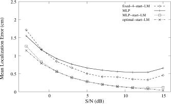
Mean localization error vs. SNR. MLP, MLP‐start‐LM, and optimal‐start‐LM were tested on signals from 25,000 random dipoles, contaminated by real brain noise.
A grand summary, averaged across various SNR conditions, is shown in Table II. The trained MLP is fastest, and its hybrid system is about 40× faster than is random‐20‐start‐LM, whereas the hybrid system is about 9× faster, yet more accurate, than is fixed‐4‐start‐LM. This means that MLP‐start‐LM was about twice as fast as might be expected naively.
Table II.
Comparison of performances on real brain noise test set of LM source localizers with three LM restart strategies, the trained MLP, and a hybrid system
| Algorithm | Computation time (ms) | Localization error (cm) |
|---|---|---|
| Fixed‐4‐start‐LM | 120 | 0.83 |
| Random‐20‐start‐LM | 663 | 0.54 |
| Optimal‐start‐LM | 14 | 0.49 |
| MLP | 0.7 | 0.90 |
| MLP‐start‐LM | 15 | 0.53 |
Each number is an average over 25,000 localizations, so error bars are negligible. Training used real brain noise.
LM, Levenberg‐Marquart; MLP, multilayer perceptron
Localization on Real MEG Signals and Comparison With Commercial Software
The sensors in MEG systems have poor SNRs for single‐trial data, because MEG data is contaminated strongly by various noises. BSS of MEG data segregates noise from signal [Sander et al., 2002; Tang et al., 2000a; Vigário et al., 2000], raising the SNR sufficiently to allow single‐trial analysis [Tang et al., 2000b]. Although the sensor attenuation vectors of BSS‐separated components can be localized well to equivalent current dipoles [Tang et al., 2002; Vigário et al., 2000], the recovered field maps can be quite noisy. We applied the MLP and MLP‐start‐LM to localize single dipolar sources from various actual BSS‐separated MEG signals. The XFIT program (standard commercial software bundled with the 4D Neuroimaging Neuromag‐122 MEG system, generally operated with some manual assistance) is compared to the methods developed here. The MEG signal processing pipeline we used is depicted in Figure 6.
Figure 6.

MEG source localization procedure.
Continuous 122‐channel MEG data for four subjects was collected using a cognitive protocol, band‐pass filtered, separated using second‐order blind identification algorithm (SOBI), and scanned for neuronal sources of interest. For each subject, four visual reaction experiments6 were carried out on the same day, but each in a separate session. Subjects were permitted to move their heads between experiments. SOBI was carried out on continuous 122‐channel data collected during the entire period of the experiment to generate 122 components, each a 1D time series with an associated field map (attenuation vector in Figure 6). Each component potentially corresponds to a set of magnetic field generators. The input to the dipole‐fitting algorithm of XFIT was the attenuation vector and the output was the location of equivalent current dipoles. From all separated components for four subjects and four tasks shown in the Appendix, we chose (using the procedures of [Tang et al., 2002]) the 14 BSS‐separated MEG signal components for which XFIT had localized a single dipole source well and that matched other criteria7 for correct localization (see Appendix for further experimental details).
The field map of each separated component was scaled to an RMS of 0.5 and input to the trained MLP. The MLP outputs were transformed from MLP output coordinates to head coordinates, and these dipole locations were used to initialize a LM routine. For each component, three results (XFIT, trained MLP, and MLP‐start‐LM) were compared. Figure 7 shows the dipoles localized by the MLP, hybrid MLP‐start‐LM, and XFIT, for four BSS‐separated MEG signal components from the trump card task of Subject S01, and Figure 8 shows the localized dipoles for three BSS‐separated MEG signal components from the transverse patterning task of Subject S01. Each figure consists of three viewpoints: axial (x–y plane), coronal (x–z plane), and sagittal (y–z plane).
Figure 7.

Dipole source localization results of Neuromag software (XFIT), our MLP, and MLP‐start‐LM for four real BSS‐separated MEG signal components obtained in the trump card task of Subject 1. Left, axial view; center, coronal view; right, sagittal view. The outer surface denotes the sensor surface, and diamonds on this surface denote sensors. The inner surface denotes a spherical head model fit to the subject. The center of a fitted spherical head model is (0.335, 0.698, 3.157). All units are in cm. Each localized dipole source triple is denoted by an acronym: PV, primary visual source; SV, secondary visual source; RA, auditory source in the right hemisphere; LA, auditory source in the left hemisphere.
Figure 8.

Dipole source localization results of Neuromag software (XFIT), our MLP, MLP‐start‐LM for real BSS‐separated MEG signal components obtained by transverse patterning task of Subject 1. The center of a fitted spherical head model is at (0.373, 0.642, 3.205). Layout as in Figure 7. Each localized dipole source triple is denoted by an acronym: PV, primary visual source; SV, secondary visual source; RS, somatosensory source in the right hemisphere.
Figures 9, 10, 11 show the dipole locations estimated by the MLP, MLP‐start‐LM, and Neuromag XFIT software, for various sensory sources (primary visual sources, secondary visual sources, and auditory sources) over four tasks in subject S01. Figure 12 shows the estimated dipole locations for somatosensory sources over three different subjects. All dipole locations estimated by the MLP and MLP‐start‐LM are clustered within ∼ 3 cm, and ∼ 0.7 cm, of XFIT's results, respectively. We see that the primary visual sources are localized more consistently than are the secondary visual sources, across all four tasks. The secondary sources also had more variable stimulus‐locked average time courses [Tang and Pearlmutter, 2003]. It is noticeable that somatosensory sources in the right hemisphere are localized poorly by the MLP, but well localized by the hybrid method. Although the auditory sources are the weakest, i.e., have the lowest SNRs, they are reasonably well localized.
Figure 9.

Dipole source localization results of Neuromag software (XFIT), our MLP, and MLP‐start‐LM, for four BSS‐separated primary visual MEG signal components from Subject S01, taken from four tasks. Dipole locations are shown full‐scale in the top row, whereas graphs on the bottom zoom in on the rectangular regions shown. Layout as in Figure 7.
Figure 10.

Dipole source localization results of Neuromag software (XFIT), our MLP, and MLP‐start‐LM for four BSS‐separated secondary visual MEG signal components from Subject S01, over four tasks. Dipole locations are shown full‐scale in the top row, whereas graphs on the bottom zoom in on the rectangular regions shown. Layout as in Figure 7.
Figure 11.

Dipole source localization results of Neuromag software (XFIT), our MLP, and MLP‐start‐LM for three real BSS‐separated auditory MEG signal components from Subject S01, over the trump card (TCT) and elemental discrimination (EDT) tasks. Dipole locations are shown full‐scale in the top row, whereas graphs on the bottom zoom in on the rectangular regions shown. Layout as in Figure 7.
Figure 12.

Dipole source localization results of Neuromag software (XFIT), our MLP, and MLP‐start‐LM for three BSS‐separated somatosensory MEG signal components from the transverse patterning task (TPT) over three subjects (S01, S02, S03). Dipole locations are shown full‐scale in the top row, whereas graphs on the bottom zoom in on the rectangular regions shown. Layout as in Figure 7.
Although the MLP‐estimated location is about 1.16 cm (|dx| ≈ 0.90, |dy| ≈ 0.57, |dz| ≈ 0.46) on average (N = 14) from those of XFIT, the hybrid method's result is about 0.35 cm (|dx| ≈ 0.20, |dy| ≈ 0.22, |dz| ≈ 0.10) from the location estimated by XFIT. A total of 14 localization results by both the MLP and MLP‐start‐LM are summarized in Table III. Considering that XFIT had extra information, namely the identity of a subset of the sensors to use, this hybrid method result is believed to be almost as good as the XFIT result. The trained MLP and the hybrid method are applicable to actual MEG signals, and seem to offer comparable localization relative to XFIT, with clear advantages in speed and in the lack of required human interaction or subjective human input.
Table III.
Dipole locations calculated by MLP and MLP‐start‐LM relative to XFIT's estimate, for 14 actual BSS‐separated MEG signal components
| Subject | Task | Brain activity | MLP (cm) | MLP‐start‐LM (cm) | ||||
|---|---|---|---|---|---|---|---|---|
| dx | dy | dz | dx | dy | dz | |||
| S01 | SPT | PV | −0.09 | −0.44 | 0.24 | −0.01 | −0.03 | −0.01 |
| SV | 2.74 | −0.71 | 0.39 | 0.55 | 0.20 | −0.17 | ||
| TCT | PV | 0.16 | 0.32 | −0.28 | −0.04 | 0.40 | −0.22 | |
| SV | 1.65 | −0.24 | 0.22 | 0.55 | 0.34 | −0.04 | ||
| RA | 0.03 | −0.30 | −0.07 | 0.00 | 0.05 | 0.13 | ||
| LA | 0.63 | 0.46 | −0.48 | 0.12 | 0.40 | 0.02 | ||
| EDT | PV | −0.03 | −0.02 | 0.34 | 0.01 | 0.12 | 0.00 | |
| SV | 1.37 | −0.04 | 0.35 | 0.44 | 0.23 | −0.04 | ||
| LA | 0.14 | 0.20 | −0.25 | −0.15 | 0.57 | −0.35 | ||
| TPT | PV | −0.21 | −0.52 | 0.30 | −0.12 | 0.28 | −0.03 | |
| SV | 1.32 | −0.30 | −0.17 | 0.29 | 0.22 | 0.03 | ||
| RS | −1.05 | −1.43 | 0.75 | −0.18 | 0.03 | −0.20 | ||
| S02 | TPT | RS | −1.82 | −1.43 | 1.27 | −0.19 | −0.10 | 0.01 |
| S03 | TPT | RS | −1.37 | −1.52 | 1.29 | −0.11 | −0.05 | 0.11 |
MLP, multilayer perceptron; LM, Levenberg‐Marquardt source localizers; BSS, blind source separated; MEG, magnetoencephalography; SPT, stimulus pre‐exposure task; TCT, trump cart task; ECT, elemental discrimination task; TPT, transverse patterning task; PV, primary visual source; SV, secondary visual source; RA, auditory source in the right hemisphere; LA, auditory source in the left hemisphere; RS, somatosensory source in the left hemisphere.
Assumptions and Limitations
Because the MLP outputs a particular source hypothesis, rather than a posterior distribution of hypotheses, error bars cannot be generated easily. Furthermore, the MLP is only intended as a single stage in a data processing pipeline. Its performance is hence limited by the performance of previous stages. In particular, the MLP is trained using field maps generated by a forward model, and after training takes as input noisy field maps presumed to originate from a main focal source. Consequently, it is necessary to assume that an accurate forward model is available to generate training data, and that field maps corresponding to focal sources can be gleaned from acquired data. Before the output of the MLP could be trusted, these two assumptions would need to have been tested. Fortunately, the two assumptions have been the subject of extensive investigation. The accuracy of forward models has been estimated using both phantom studies [Baillet et al., 2001; Kraus et al., 2002; Leahy et al., 1998] and experiments designed to activate known focal brain regions [Balish et al., 1991; Barth et al., 1986]. Although averaging and manual peak‐picking is the most common technique for generating field maps from acquired data, we are interested in integration with fully automated methods. One such technique that we have used is blind source separation (BSS). BSS has been shown to segregate neuronal from nonneuronal signals, and neuronal signals from each other, in both EEG [Jung et al., 2000a, b; Makeig et al., 1997, 1999] and MEG [Cao et al., 2000; Tang et al., 2000a, b, 2002; Tang and Pearlmutter, 2003; Vigário et al., 1998, 1999, 2000; Wübbeler et al., 2000; Ziehe et al., 2000]. For these reasons, despite its limitations, it seems feasible to use the localizer proposed above as a stage in a practical robust real‐time MEG processing pipeline.
CONCLUSIONS
We propose the inclusion of a head position input for MLP‐based MEG dipole localizers. This overcomes the limitation of previous MLP‐based MEG localization systems, namely the need to retrain the network for each session or subject. Experiments showed that the trained MLP was far faster, albeit slightly less accurate, than was fixed‐4‐start‐LM. This motivated us to construct a hybrid system, MLP‐start‐LM, which improves localization accuracy while reducing the computational burden to less than one‐ninth that of fixed‐4‐start‐LM. This hybrid method was comparable in accuracy to random‐20‐start‐LM, at 1/40th the computation burden, which is about two times faster than might be expected naively. Over the whole range of SNRs, the hybrid system showed almost as good performance in accuracy and computation time as that with hypothetical optimal‐start‐LM.
We applied the MLP and MLP‐start‐LM to localize single dipolar sources from actual BSS‐separated MEG signals, and compared these to the results of the commercial Neuromag program XFIT. The MLP yielded dipole locations close to those of manually assisted XFIT, and MLP‐start‐LM gave locations that were even closer to those of XFIT.
In conclusion, this MLP can itself serve as a reasonably accurate real‐time MEG dipole localizer, even when the head position changes regularly. This MLP also constitutes an excellent initializer for LM, coming very close to meeting the Cramer‐Rao bound in this role. Because the MLP receives a head position input, a weakness of all previous MLP‐based systems, namely the need to retrain for various subjects or sessions, has been eliminated without sacrificing the advantages of the universal‐approximator direct inverse approach to localization. In other words, for a particular MEG system, this network needs to be trained only once.
The most serious weakness of the system presented above is its inability to localize automatically multiple dipoles from a single field map. We hope to overcome this limitation by combining the subject‐independent approach described above with the distributed output representation used in earlier work [Jun et al., 2003] and introducing a post‐processing clustering phase.
Acknowledgements
We thank G. Nolte for help with the forward model, M. Weisend for allowing us to use his data, and M. Weisend, A. Tang, and N. Malaszenko for providing experimental details.
MLP structure
The MLP charged with approximating the inverse mapping had an input layer of 125 units consisting of the three Cartesian coordinates of the center of a fitted sphere and the 122 sensor activations (Fig. 13). It had two hidden layers with N 1 = 320 and N 2 = 30 units, respectively, and an output layer of three units representing the Cartesian coordinates of the fitted dipole.8
Figure 13.

Training datasets were loaded into this MLP structure. Note that the input includes the coordinates of the center of a sphere fit to the subject's head.
As in [Jun et al., 2002], the output units had linear activation functions,9 whereas to accelerate training the hidden unit had hyperbolic tangent activation functions [LeCun et al., 1991]. As shown in Figure 6, adjacent layers were connected fully, and there were no cut‐through connections. Input data are usually preprocessed to improve performance, and output data is scaled into the dynamic range of the output unit activation function to avoid driving the weights of the network to infinity or driving the hidden units to saturation [Abeyratne et al., 1991; Haykin, 1994]. The 122‐sensor activation inputs were scaled to an RMS value of 0.5, and the target outputs were scaled into the region (−1, +1). The network weights were initialized with uniformly distributed random values between ±1. Backpropagation was used to calculate the gradient [Rumelhart et al., 1986], and online stochastic gradient descent with no momentum (the past increment to the weights) was used for optimization, with the learning rate (constant of proportionality for weights updates) chosen empirically.
Experimental Details
Continuous 300 Hz MEG data for four right‐handed subjects (two females, two males) was collected using a cognitive protocol developed by Michael P. Weisend, band‐pass filtered at 0.03–100 Hz, separated using the second‐order blind identification algorithm (SOBI), and scanned for neuronal sources of interest. In all tasks, each trial consisted of a pair of colored abstract block compositions, of which one was the target presented symmetrically and simultaneously on the left and right halves of the screen. When a target stimulus was presented to the left or right side of the screen, respectively, subjects were instructed to respond with a left‐ or right‐hand mouse press. The button press elicited an auditory feedback that was composed of two sorts of tones indicating correct versus incorrect choices. For each subject, all four experiments were carried out on the same day, but each in a separate session. Subjects were permitted to move their heads between experiments. The following four visual reaction time tasks were carried out by each subject:
Stimulus pre‐exposure task (SPT):
There were no predefined relationships between stimuli and button presses. No feedback was given to the subjects about any choice. Trump card task (TCT): Subjects were instructed to discover, by trial and error, which of the two stimuli in the stimulus pair was the target (the trump card). A total of 9 stimulus pairs involving 10 stimuli were used, with a single stimulus as the trump card.
Elemental discrimination task (EDT):
Subjects were instructed to discover which one of the stimulus pair was the target stimulus by trial and error. A total of three stimulus pairs consisting of six stimuli were used. For each pair of stimuli, one of the pair was the target.
Transverse patterning task (TPT):
Subjects were instructed to discover which of the two stimuli in a stimulus pair was the target. Three stimulus pairs consisting of three stimulus compositions were used. Each stimulus could be a target or nontarget depending upon what it was paired with.
SOBI was carried out on continuous 122‐channel data collected during the entire period of the experiment. It generated 122 components, each a 1D time series with an associated field map. Each component potentially corresponds to a set of magnetic field generators. Event‐triggered averages were calculated from their continuous single‐trial time series for all 122 separated components, where the triggering events were either sensory stimuli or behavioral responses. For a task‐related component, if its field map and time course were consistent with known neurophysiologic and neuroanatomic facts, we considered it a neural component reflecting the activity of a neuronal generator. A dipole‐fitting method was applied to the identified neural components. The input to the dipole‐fitting algorithm of XFIT was the field map and the output was the location of ECDs projected onto the subject's structural MRI images. See [Tang et al., 2002] for further experimental details along with a more detailed description of the SOBI algorithm.
Footnotes
Given the sensor activations and a dipole location, the minimum error dipole moment can be calculated analytically [Hämäläinen et al., 1993]. Although the dipoles used in generating the dataset had both location and moment, the moments were therefore not included in the datasets used for training or testing.
Fitted spheres from 12 subjects carrying out various tasks on a 4D Neuroimaging Neuromag‐122 MEG system were collected, and this distribution of head positions was chosen to include all 12 cases. Just as the position of the center of the head varies from session to session and subject to subject, so does head orientation and radius. Because a sphere is rotationally symmetric, our forward model is insensitive to orientation, and similarly the external magnetic field caused by a dipole in a homogeneous sphere is invariant to the sphere's radius. On the other hand, the noise process would not be invariant to orientation or radius, so we might expect a slight increase in performance if the network had orientation and radius available as inputs, rather than just the position of the center.
This allowed only tangential components.
In one epoch each exemplar in the training dataset is presented once.
These tuned initial points were chosen empirically and manually, using simulations and repeated trial‐and‐error, to roughly optimize localization performance.
Stimulus pre‐exposure task (SPT), Trump card task (TCT), Elemental discrimination task (EDT), and Transverse patterning task (TPT). For more detail, see Appendix.
Source field maps, time courses, and localized dipoles were checked for consistency with known neurophysiology and anatomy [Tang et al., 2002].
After Jun et al. [ 2002], we used N 1 = 320 and N 2 = 30 units for the two hidden layers. Slightly better performance might be expected if the number of units in the hidden layers were optimized for this particular application.
In artificial neural networks, the activation function computes the output value of an artificial neuron based on the weighted sum of its inputs. The output value may be continuous or discrete, and heavyside, linear, sigmoid, and hyperbolic tangent activation functions are widely used.
REFERENCES
- Abeyratne UR, Kinouchi Y, Oki H, Okada J, Shichijo F, Matsumoto K (1991): Artificial neural networks for source localization in the human brain. Brain Topogr 4: 3–21. [DOI] [PubMed] [Google Scholar]
- Ahonen AI, Hämäläinen MS, Knuutila JET, Kajola MJ, Laine PP, Lounasmaa OV, Parkkonen LT, Simola JT, Tesche CD (1993): 122‐channel SQUID instrument for investigating the magnetic signals from the human brain. Physica Scripta 49: 198–205. [Google Scholar]
- Baillet S, Riera JJ, Marin G, Mangin JF, Aubert J, Garnero L (2001): Evaluation of inverse methods and head models for EEG source localization using a human skull phantom. Phys Med Biol 46: 77–96. [DOI] [PubMed] [Google Scholar]
- Balish M, Sato S, Connaughton P, Kufta C (1991): Localization of im‐planted dipoles by magnetoencephalography. Neurology 41: 1072–1076. [DOI] [PubMed] [Google Scholar]
- Barth DS, Sutherling W, Broffman J, Beatty J (1986): Magnetic localization of a dipolar current source implanted in a sphere and a human cranium. Electroencephalogr Clin Neurophysiol 63: 260–273. [DOI] [PubMed] [Google Scholar]
- Cao JT, Murata N, Amari S, Cichocki A, Takeda T, Endo H, Harada N (2000): Single‐trial magnetoencephalographic data decomposition and localization based on independent component analysis approach. IEICE Trans Fundam Electron Commun Comput Sci 83: 1757–1766. [Google Scholar]
- de Munck JC, de Jongh A, van Dijk BW (2001): The localization of spontaneous brain activity: an efficient way to analyze large data sets. IEEE Trans Biomed Eng 48: 1221–1228. [DOI] [PubMed] [Google Scholar]
- Hämäläinen M, Hari R, Ilmoniemi RJ, Knuutila J, Lounasmaa OV (1993): Magnetoencephalography—theory, instrumentation, and applications to noninvasive studies of the working human brain. Rev Mod Phys 65: 413–497. [Google Scholar]
- Haykin SS. (1994): Neural networks: a comprehensive foundation. New York, NY: Macmillan. [Google Scholar]
- Hoey GV, Clercq JD, Vanrumste B, de Walle RV, Lemahieu I, D'Havé M, Boon P (2000): EEG dipole source localization using artificial neural networks. Phys Med Biol 45: 997–1011. [DOI] [PubMed] [Google Scholar]
- Huang MX, Mosher JC, Leahy RM (1999): A sensor‐weighted overlapping‐sphere head model and exhaustive head model comparison for MEG. Phys Med Biol 44: 423–440. [DOI] [PubMed] [Google Scholar]
- Jun SC, Pearlmutter BA, Nolte G (2002): Fast accurate MEG source localization using a multilayer perceptron trained with real brain noise. Phys Med Biol 47: 2547–2560. [DOI] [PubMed] [Google Scholar]
- Jun SC, Pearlmutter BA, Nolte G (2003): MEG source localization using a MLP with a distributed output representation. IEEE Trans Biomed Eng 50: 786–789. [DOI] [PubMed] [Google Scholar]
- Jung TP, Humphries C, Lee TW, McKeown MJ, Iragui V, Makeig S, Sejnowski TJ (2000a): Removing electroencephalographic artifacts by blind source separation. Psychophysiology 37: 163–178. [PubMed] [Google Scholar]
- Jung TP, Makeig S, Westerfield M, Townsend J, Courchesne E, Sejnowski TJ (2000b): Removal of eye activity artifacts from visual event‐related potentials in normal and clinical subjects. Clin Neurophysiol 111: 1745–1758. [DOI] [PubMed] [Google Scholar]
- Kamijo K, Kiyuna T, Takaki Y, Kenmochi A, Tanigawa T, Yamazaki T (2001): Integrated approach of an artificial neural network and numerical analysis to multiple equivalent current dipole source localization. Front Med Biol Eng 10: 285–301. [DOI] [PubMed] [Google Scholar]
- Kinouchi Y, Ohara G, Nagashino H, Soga T, Shichijo F, Matsumoto K (1996): Dipole source localization of MEG by BP neural networks. Brain Topogr 8: 317–321. [DOI] [PubMed] [Google Scholar]
- Kraus RH Jr, Volegov PL, Maharajh K, Espy MA, Matlashov AN, Flynn ER (2002): Performance of a novel SQUID‐based superconducting imaging‐surface magnetoencephalography system. Physica C 368: 18–23. [Google Scholar]
- Kwon HC, Lee YH, Jun SC, Kim JM, Park JC, Kuriki S (2000): Localization errors with 40‐channel tangential fields In: Nenonen J, Ilmoniemi RJ, Katila T, editors. Biomag2000. Proc 12th Int Conf on Biomagnetism. Espoo, Finland: Helsinki University of Technology; p 943–946. [Google Scholar]
- Kwon H, Lee YH, Kim JM, Park YK, Kuriki S (2002): Localization accuracy of single current dipoles from tangential components of auditory evoked fields. Phys Med Biol 47: 4145–4154. [DOI] [PubMed] [Google Scholar]
- Leahy RM, Mosher JC, Spencer ME, Huang MX, Lewine JD (1998): A study of dipole localization accuracy for MEG and EEG using a human skull phantom. Electroencephalogr Clin Neurophysiol 107: 159–173. [DOI] [PubMed] [Google Scholar]
- LeCun Y, Kanter I, Solla SA (1991): Second‐order properties of error surfaces: learning time and generalization In: Lippmann R, Moody J, Touretzky D, editors. Advances in neural information processing systems 3 Denver, CO: Morgan Kaufmann; p 918–924. [Google Scholar]
- Levenberg K (1944): A method for the solution of certain problems in least squares. Q Appl Math 2: 164–168. [Google Scholar]
- Makeig S, Jung TP, Bell AJ, Ghahremani D, Sejnowski TJ (1997): Blind separation of auditory event‐related brain responses into independent components. Proc Natl Acad Sci USA 94: 10979–10984. [DOI] [PMC free article] [PubMed] [Google Scholar]
- Makeig S, Westerfield M, Jung TP, Covington J, Townsend J, Sejnwoski TJ, Courchesne E (1999): Functionally independent components of the late positive event‐related potential during visual spatial attention. J Neurosci 19: 2665–2680. [DOI] [PMC free article] [PubMed] [Google Scholar]
- Marquardt DW (1963): An algorithm for least‐squares estimation of nonlinear parameters. SIAM J Appl Math 11: 431–441. [Google Scholar]
- Nolte G (2004): The magnetic lead field theorem in the quasi‐static approximation and its use for MEG forward calculation in realistic volume conductors. Phys Med Biol 48: 3637–3652. [DOI] [PubMed] [Google Scholar]
- Nolte G, Fieseler T, Curio G (2000): Perturbation theory as a new analytical approach to the MEG forward problem for realistic volume conductor modeling of the head In: Nenonen J, Ilmoniemi R, Katila T, editors. Biomag2000. Proc 12th Int Conf on Biomagnetism. Espoo, Finland: Helsinki University of Technology; p 623–626. [Google Scholar]
- Rumelhart DE, Hinton GE, Williams RJ (1986): Learning representations by back‐propagating errors. Nature 323: 533–536. [Google Scholar]
- Sander TH, Wübbeler G, Lueschow A, Curio G, Trahms L (2002): Cardiac artifact subspace identification and elimination in cognitive MEG data using time‐delayed decorrelation. IEEE Trans Biomed Eng 49: 345–354. [DOI] [PubMed] [Google Scholar]
- Sarvas J (1987): Basic mathematical and electromagnetic concepts of the biomagnetic inverse problem. Phys Med Biol 32: 11–22. [DOI] [PubMed] [Google Scholar]
- Sun M, Sclabassi RJ (2000): The forward EEG solutions can be computed using artificial neural networks. IEEE Trans Biomed Eng 47: 1044–1050. [DOI] [PubMed] [Google Scholar]
- Tang AC, Pearlmutter BA, Zibulevsky M, Carter SA (2000a): Blind separation of multichannel neuromagnetic responses. Neurocomputing 32–33: 1115–1120. [Google Scholar]
- Tang AC, Pearlmutter BA, Zibulevsky M, Hely TA, Weisend MP (2000b): An MEG study of response latency and variability in the human visual system during a visual‐motor integration task In: Solla SA, Leen TK, Müller KR, editors. Advances in neural information processing systems 12 Cambridge, MA: MIT Press; p 185–191. [Google Scholar]
- Tang AC, Pearlmutter BA, Malaszenko NA, Phung DB, Reeb BC (2002): Independent components of magnetoencephalography: localization. Neural Comput 14: 1827–1858. [DOI] [PubMed] [Google Scholar]
- Tang AC, Pearlmutter BA (2003): Independent components of magnetoencephalography: localization and single‐trial response onset detection In: Lu ZL, Kaufman L, editors. Magnetic source imaging of the human brain. Mahwah, NJ: Lawrence Erlbaum Associates; p 159–201. [Google Scholar]
- Vanrumste B, Van Hoey G, D'Havé M, Lemahieu I, Boon P (2002): Comparison of performance of spherical and realistic head models in dipole localization from noisy EEG. Med Eng Phys 24: 403–418. [DOI] [PubMed] [Google Scholar]
- Vigário R, Jousmäki V, Hämäläinen M, Hari R, Oja E (1998): Independent component analysis for identification of artifacts in magnetoencephalographic recordings In: Jordan MI, Kearns MJ, Solla SA, editors. Advances in neural information processing systems 10 Cambridge, MA: MIT Press; p 229–235. [Google Scholar]
- Vigário R, Särelä J, Jousmäki V, Hämäläinen M, Oja E (2000): Independent component approach to the analysis of EEG and MEG recordings. IEEE Trans Biomed Eng 47: 589–593. [DOI] [PubMed] [Google Scholar]
- Vigário R, Särelä J, Jousmäki V, Oja E (1999): Independent component analysis in decomposition of auditory and somatosensory evoked fields. In: Proc First Int Conf on Independent Component Analysis and Blind Source Separation (ICA'99) Aussois, France. p 167–172.
- Wübbeler G, Ziehe A, Mackert BM, Müller KR, Trahms L, Curio G (2000): Independent component analysis of non‐invasively recorded cortical magnetic DC‐fields in humans. IEEE Trans Biomedical Eng 47: 594–599. [DOI] [PubMed] [Google Scholar]
- Yuasa M, Zhang Q, Nagashino H, Kinouchi Y (1998): EEG source localization for two dipoles by neural networks. In: Proc 20th Ann Int Conf of the IEEE Engineering in Medicine and Biology Society. Hong Kong. p 2190–2192.
- Ziehe A, Müller KR, Nolte G, Mackert BM, Curio G (2000): Artifact reduction in magnetoneurography based on time‐delayed second order correlations. IEEE Trans Biomed Eng 47: 75–87. [DOI] [PubMed] [Google Scholar]