

Abstract
Potential-based inverse electrocardiography is a method for the noninvasive computation of epicardial potentials from measured body surface electrocardiographic data. From the computed epicardial potentials, epicardial electrograms and isochrones (activation sequences), as well as repolarization patterns can be constructed. We term this noninvasive procedure Electrocardiographic Imaging (ECGI). The method of choice for computing epicardial potentials has been the Boundary Element Method (BEM) which requires meshing the heart and torso surfaces and optimizing the mesh, a very time-consuming operation that requires manual editing. Moreover, it can introduce mesh-related artifacts in the reconstructed epicardial images. Here we introduce the application of a meshless method, the Method of Fundamental Solutions (MFS) to ECGI. This new approach that does not require meshing is evaluated on data from animal experiments and human studies, and compared to BEM. Results demonstrate similar accuracy, with the following advantages: 1. Elimination of meshing and manual mesh optimization processes, thereby enhancing automation and speeding the ECGI procedure. 2. Elimination of mesh-induced artifacts. 3. Elimination of complex singular integrals that must be carefully computed in BEM. 4. Simpler implementation. These properties of MFS enhance the practical application of ECGI as a clinical diagnostic tool.
Keywords: Method of fundamental solutions (MFS), Electrocardiographic imaging (ECGI), Meshless method, Inverse problem, Boundary element method (BEM), Electrocardiography, Cardiac arrhythmia
INTRODUCTION
Computation of potentials on the surface of the heart from potentials measured on the body surface involves solving Laplace’s equation in the source-free volume between the torso and heart surfaces. Several mathematical and computational approaches were introduced to solve this problem, known as the inverse problem of electrocardiography in terms of potentials.3,29,71,80 Other approaches have used a bi-domain model or a uniform dipole layer (UDL) to compute activation times (isochrones) on the heart surface.28,43,58,60 Recently, both the potential-based approach (for computing epicardial potentials, electrograms, and isochrones) and the activation-time approach were applied and evaluated in human subjects.28,33,47,49,57–60,65,67,77–79 Both methods require discretizing the heart and torso surfaces into continuous non-overlapping mesh elements, a procedure called meshing. Meshing is difficult to apply to irregular surfaces37 and can introduce mesh-related artifacts, especially in the computation of solutions to the ill-posed76 electrocardiographic problem, if mesh optimization is not carefully done. In most applications of inverse electrocardiography, the Boundary Element Method (BEM)5,12 was used to solve Laplace’s equation.2,49,70 In this approach, mesh optimization is the most time-consuming step and requires manual intervention and editing. Importantly, this formulation requires computation of complicated singular integrals that require careful handling.1,36,73 In addition, BEM often suffers from slow convergence due to the use of low order polynomial approximations.36,63 These difficulties with the efficient implementation of BEM led us to explore the possibility of applying a meshless method to inverse electrocardiography, in the hope of overcoming such mesh-related problems.
Meshless methods have been applied successfully in a wide array of engineering and industrial application.26,41 Inverse electrocardiography is a 3D Cauchy problem for the Laplace operator which has a very well behaved, analytic fundamental solution.42 This property suggests the Method of Fundamental Solutions (MFS)27 as the method of choice for this problem among the family of meshless methods.6 In MFS, the potential is expressed as summation over a discrete set of virtual point sources placed outside the domain of interest. A related approach31 used distributed surface charge densities on actual boundaries as sources for forward computation of potentials. This method required dense meshing of the surfaces and evaluation of singular integrals, procedures that are bypassed by MFS.
In this study, we formulate the use of MFS in inverse electrocardiography and evaluate its performance. We test this new method using data from animal experiments62 and human studies,49,67 and compare its performance to the BEM-based approach that requires meshing. Human data were processed using the potential-based method with geometrical information (heart-torso geometry) obtained noninvasively using CT imaging. All approaches to the noninvasive reconstruction of cardiac electrical activity can be referred to as cardiac electrophysiological imaging modalities. The potential-based inverse electrocardiography is a method for the noninvasive computation of epicardial potentials from measured body surface electrocardiographic data. From the computed epicardial potentials, epicardial electrograms and isochrones (activation sequences), as well as repolarization patterns can be constructed. We term this noninvasive procedure Electrocardiographic Imaging (ECGI). For clarity, we refer in the paper to MFS application in ECGI as MFS ECGI, and its BEM version as BEM ECGI.
METHODS
Formulating the Method of Fundamental Solutions for ECGI
The method of fundamental solutions (MFS) has been used in various mathematical and engineering applications to compute solutions of partial differential equations (PDE).26,41 MFS approximates the solution of a PDE by a linear combination of fundamental solutions of the governing partial differential operator,27 which for ECGI is the Laplacian operator ▽². The formulation of MFS for a▽² boundary value problem and Cauchy problem is described in the Appendix; its implementation in ECGI is described below.
The objective of ECGI is to determine the electric potential on the epicardial surface of the heart noninvasively, from measurements of the electric potential on the torso surface. This constitutes a Cauchy problem for Laplace’s equation:42
| (1) |
with the following boundary conditions:
Dirichlet condition: on the torso surface
Neumann condition: on the torso surface
where Ω is the 3D volume domain between the heart’s epicardial surface ΓE and the torso surface ΓT as shown in Fig. 1. u(x) is the potential at location x; uT(x) and cT(x) are the potential and its normal derivative on the torso surface, respectively. The goal of ECGI is to obtain the electric potential on the heart surface uE(x), x ∈ Γ E
FIGURE 1.
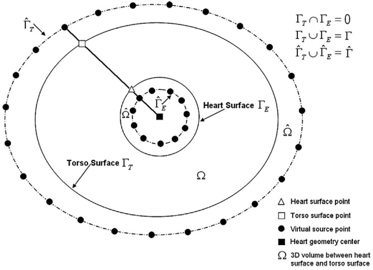
A schematic showing the configuration of fictitious points for a multi-connected domain. The dashed lines are the auxiliary surfaces that contain the fictitious points (virtual sources) marked by black circles. The filled square is the geometrical center of the “heart”, the empty triangle is located on the “heart surface” and the empty square on the “torso surface,” the two black circles on their connecting line at the auxiliary surfaces are the corresponding virtual source points.
MFS is an approach for solving numerically Laplace’s equation. In MFS, an approximate solution is represented in the form of a linear superposition of source functions (fundamental solutions) located on a set of points (fictitious points, virtual sources) over an auxiliary surface Γ̂ (Γ̂ encloses the auxiliary domain Ω̂, which contains the actual domain Ω as shown in Fig. 1). As the fundamental solutions satisfy Laplace’s equation everywhere except at source points, this representation satisfies Laplace’s equation in the domain Ω. In addition, the specified boundary conditions are imposed at a set of boundary points (collocation points) on the domain boundary Γ. Since the fundamental solutions do not have singularities at points on the boundary Γ, standard quadrature rules can be used to approximate the surface potential and its normal gradient when computed on the boundary.37
As shown in the Appendix (Eq. (a21) and Eq. (a22)), MFS can be applied to discretize the Dirichlet and Neumann boundary conditions in Eq. (1) as:
| (2) |
| (3) |
where is the fundamental solution of Laplace’s equation in 3D, r = ‖x − y‖ is the 3D Euclidean distance between point x and point y, n̂ is normal to the torso surface, a0 is the constant component of uT (x) and aj is the coefficient of a virtual source at location yj. Note that a0 and aj have different units in this formulation. The conductivity of the volume is reflected in the coefficient aj; it does not appear explicitly in the ECGI formulation when the volume of interest is homogenous. M is the number of fictitious points. N is the number of torso surface points. Γ is the boundary of domain Ω, and Γ̂ is the auxiliary boundary of the auxiliary domain Ω̂, which contains the domain Ω as shown in Fig. 1.
Boundary conditions are satisfied on N torso surface points xk. In Eq. (2) uT (xk) is the measured body surface potential at electrode position xk. In Eq. (3), cT (xk) = 0 because the torso is in air, an insulating medium that does not support current flow. The locations of the fictitious points yj are configured based on the particular domain geometry, which in ECGI is a multi-connected surface in 3D, composed of the body surface and heart surface (Γ = ΓT ∪ ΓE). Using a static configuration scheme (see Appendix), the fictitious sources are placed on two auxiliary surfaces (Γ̂ = Γ̂T ∪ Γ̂E) which are determined by inflation/deflation of the true surfaces (torso surface and heart surface). Figure 1 shows the configuration of the fictitious points in a 2D representation. The fictitious boundary corresponding to the heart surface Γ̂E is obtained by deflating the heart surface by a factor of 0.8 relative to the geometrical center of the heart. The geometrical center of the heart can be found by computing the average coordinate value of all the heart surface nodes. For the torso surface, the fictitious boundary Γ̂T is obtained by inflating the torso surface by a factor of 1.2 relative to the geometrical center of the heart.
Expressing Eq. (2) and Eq. (3) in matrix form gives:
| (4) |
Matrix  is of dimension 2N × (M + 1); and are vectors of dimensions M + 1 and 2N respectively.
This matrix equation can not be solved for without regularizaiton,76 because the matrix  is ill-conditioned and the measured body surface potential contains measurement error. The Tikhonov regularization method76 with CRESO-determined regularization parameter24 is used to stabilize the inverse procedure and obtain , similar to our previous ECGI inverse computations using mesh-based BEM.15,16,32,33,47,56,61,62,65–71
Once the coefficient vector is obtained, u(x) can be computed at any location in the domain using:
| (5) |
The epicardial potential can then be calculated using:
| (6) |
Epicardial potentials are calculated using (6) on many epicardial nodes; numbers are provided for each dataset in the Results section. An epicardial potential map, reflecting the spatial distribution of potentials on the epicardial surface, is computed every millisecond during the cardiac cycle. The time series of reconstructed epicardial potential maps are then organized by location to provide temporal electrograms for any given point on the epicardium. A reconstructed epicardial electrogram provides the potential variation with time at a given point on the epicardium during the cardiac cycle. Epicardial isochrone maps (a map of the epicardial activation sequence) are computed by taking the time of maximum negative of the temporal electrogram (“intrinsic deflection”) at a given location as the time of epicardial activation at that location.
Experimental Methods and Protocols
MFS ECGI reconstructions were performed on data from four studies: (i) Single-site pacing in an isolated canine heart suspended in a human torso-shaped tank; data were obtained during pacing from a right ventricular (RV) anterior epicardial location;62 (ii) RV endocardial pacing in a patient undergoing bi-ventricular pacing for cardiac resynchronization therapy (CRT); (iii) Simultaneous RV endocardial pacing and left ventricular (LV) epicardial pacing in a patient undergoing bi-ventricular pacing for CRT; (iv) Normal atrial activation in a healthy human subject.65
Isolated Canine Hearts Suspended in a Human Torso-Shaped Tank62
The performance of MFS in ECGI was evaluated using data from a human torso-shaped tank.62 The setup consisted of an isolated canine heart suspended in a homogenous electrolytic medium in the correct anatomical position inside a tank molded in the shape of a ten-year old boy. The tank had 384 surface electrodes recording torso potentials and 242 rods with electrodes at their tips that formed an epicardial recording envelope around the heart. The complete sets of torso-surface potentials and epicardial potentials were obtained by recording over several beats. The directly measured epicardial potentials by the rod-tip electrodes served as a “gold standard” for MFS ECGI validation. The torsosurface potentials provided the input data for MFS ECGI noninvasive reconstruction of epicardial potentials, electrograms and isochrones, which were then evaluated by comparison with the directly measured “gold standard”. Details were provided in previous ECGI publications.15,61,62,70
To simulate focal arrhythmogenic activity, the heart was paced from an anterior epicardial location. The same datasets were used in BEM ECGI and reported in previous publications.62 Here, these datasets are used to evaluate MFS ECGI and compare its performance to that of BEM ECGI. The pacing protocol also provided a measure of MFS ECGI spatial accuracy (its accuracy in locating the known pacing site). After pacing, a quasi-elliptical region of intense epicardial negativity forms around the pacing site.61,62,70,74
Bi-Ventricular Pacing In Human Subjects65
We also applied MFS ECGI to clinical data from patients with an implanted bi-ventricular pacing device. For the biventricular pacing data, MFS ECGI accuracy in locating the pacing sites was evaluated by comparison with the pacing electrodes’ positions as determined from CT images. The reconstructed activation pattern was evaluated based on the known patterns of activation generated by pacing.
Data from two heart failure patients undergoing cardiac resynchronization pacing therapy65 are presented. Subject 1 was paced from a right ventricular (RV) endocardial site, close to the RV apex. Subject 2 was paced simultaneously from an RV endocardial site and from a left ventricular (LV) epicardial site. Body surface potentials were recorded with a 224-channel mapping system using an electrode-vest as previously described.65 Epicardial geometry and location of the torso electrodes were obtained from CT images of the thorax. The locations of the cardiac pacing leads were also determined from these CT images.65
Normal Atrial Activation in a Healthy Human Subject65
MFS ECGI was applied to reconstruct atrial activation in a healthy young adult. The same data were used in BEM ECGI and reported in a previous study.65 The atrial activation pattern was reconstructed from recorded P-wave body surface potential maps with 224 channels, together with a subject-specific torso and atrial geometry obtained using CT. The directly measured normal atrial activation pattern in isolated human hearts (Durrer et al.25), was used for qualitative evaluation of the MFS ECGI reconstruction.
Informed consent was obtained according to Institutional Review Board guidelines at University Hospitals of Cleveland, which approved all human studies protocols.
Evaluation Procedures
For the tank-torso protocols, measures in terms of relative error (RE) and correlation coefficients (CC) were computed with respect to the measured data to quantitatively evaluate the accuracy of ECGI; RE and CC were defined previously.71 RE gives an estimate of the amplitude difference and CC gives an estimate of the similarity of potential patterns or electrogram morphologies between the measured and computed data:
For potential maps, L is the number of epicardial points at which potentials are measured and computed. is the computed potential at epicardial point i, at a given instant of time, and is the corresponding measured potential. and are the spatial average of measured and computed potentials respectively, averaged over all L points.
For electrograms, L is the number of time frames for which potential is measured and computed. is the computed potential at time i, at a given epicardial location, and is the corresponding measured potential. and are the temporal average of measured and computed potentials respectively, averaged over all L times.
In addition to CC and RE, pacing site localization errors (distance between reconstructed and measured locations) were also computed for both torso-tank and human reconstructions. The reconstructed pacing site location was estimated by the center of an ellipse that best fits the quasi-elliptical negative potential region that develops around the pacing site.61,62,70 The earliest time frame after pacing, for which such pattern was present, was used for this purpose. Pacing sites could also be determined from isochrone maps as the sites of earliest activation.
Qualitative evaluations of ECGI reconstructions are conducted by visual comparison to measured data (torso-tank experiments) and to well established potential, electrogram and isochrone patterns associated with pacing and normal atrial activation (human subjects).
RESULTS
Single Site Pacing in a Torso-Shaped Tank
Figure 2 shows epicardial potential maps for anterior RV pacing, at a time 25 ms after pacing. There are 240 epicardial nodes, 386 torso nodes and 626 (240 + 386) virtual source points in this dataset. The top row shows the directly measured epicardial potential maps in four views. The middle and bottom rows show MFS-reconstructed and BEM-reconstructed epicardial potential maps, respectively. The white asterisk in the anterior view marks the pacing site location (top row) and its estimation from the reconstructed epicardial potential maps in the middle and bottom rows. The measured potentials display a central quasi-elliptical negative region (blue) flanked by two positive regions (red, maxima locations are marked by the white plus signs) as expected in the anisotropic myocardium.62,74 This pattern is captured by both BEM ECGI and MFS ECGI. However, MFS ECGI provides a more accurate potential map pattern than BEM ECGI. MFS ECGI locates the pacing site with an error of 3 mm as compared to a 5 mm error for BEM ECGI. CC (a measure of pattern similarity to the measured potentials) is improved from 0.85 (BEM ECGI) to 0.92 (MFS ECGI); RE (indicative of amplitude accuracy) is improved from 0.97 (BEM ECGI) to 0.47 (MFS ECGI).
FIGURE 2.
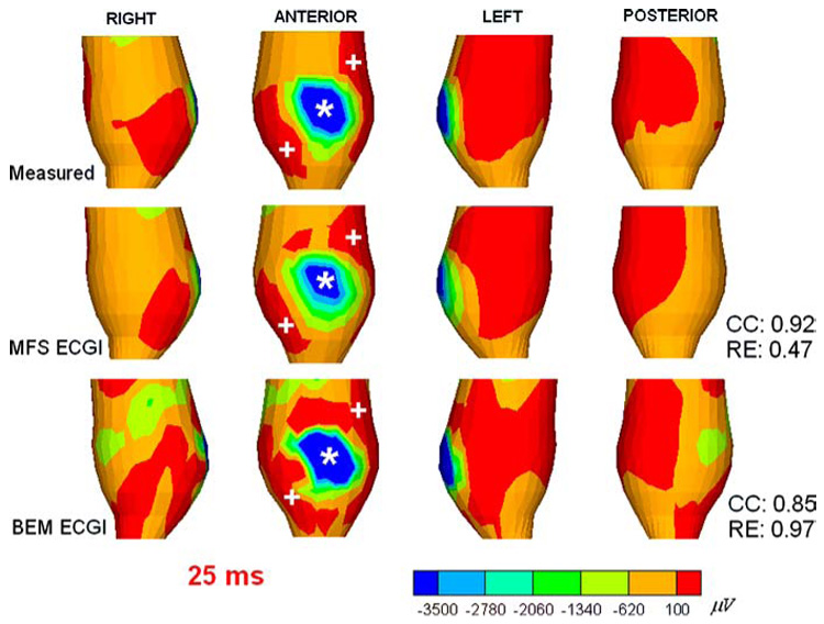
Canine epicardial potential maps 25 ms after pacing from a single anterior site (indicated by the asterisk *). Top row shows the directly measured epicardial potentials (four views) displaying the negative region (dark blue) around the pacing site, and two flanking positive maxima (red). Middle rows shows the noninvasively reconstructed potentials computed using MFS ECGI; note close similarity of noninvasive and invasive data. Bottom row shows the reconstruction using BEM ECGI.
Figure 3 shows noninvasively reconstructed epicardial electrograms (format described in figure legend) using MFS ECGI. Figure 3A shows four views of the heart surface. Electrograms reconstructed at epicardial sites close to pacing site (sites 1, 2, 3), at intermediate distance from the pacing site (sites 4, 5, 6), and far way from the pacing site (sites 7, 8, 9) are displayed. In panels B, C, and D, both measured and noninvasively computed electrograms using MFS are displayed. Three main types of waveforms: monophasic negative (B), biphasic (C), and monophasic positive (D), are reconstructed. Notice the close resemblance (high Correlation Coefficient, CC) of the noninvasively reconstructed MFS ECGI electrograms to the measured electrograms. Compared with reconstructed electrograms using BEM ECGI,62 MFS ECGI achieves better accuracy with greatly reduced computation time. Figure 4 shows noninvasively reconstructed epicardial isochrones using MFS ECGI and BEM ECGI. Notice that the region of earliest activation (red) is reproduced accurately in the computed isochrones, as is the entire sequence of epicardial activation (CC=0.78). A similar epicardial isochrone map is reconstructed by BEM ECGI (CC=0.74). Based on Fig. 4, it appears that MFS reconstructs smoother isochrones than BEM. A comparison of patterns shows closer similarity of the MFS reconstruction to the measured data, suggesting that the BEM reconstruction is somewhat under-regularized with the chosen CRESO regularization parameter. Similar observations apply to the ECGI reconstructed potential maps in Fig. 2.
FIGURE 3.
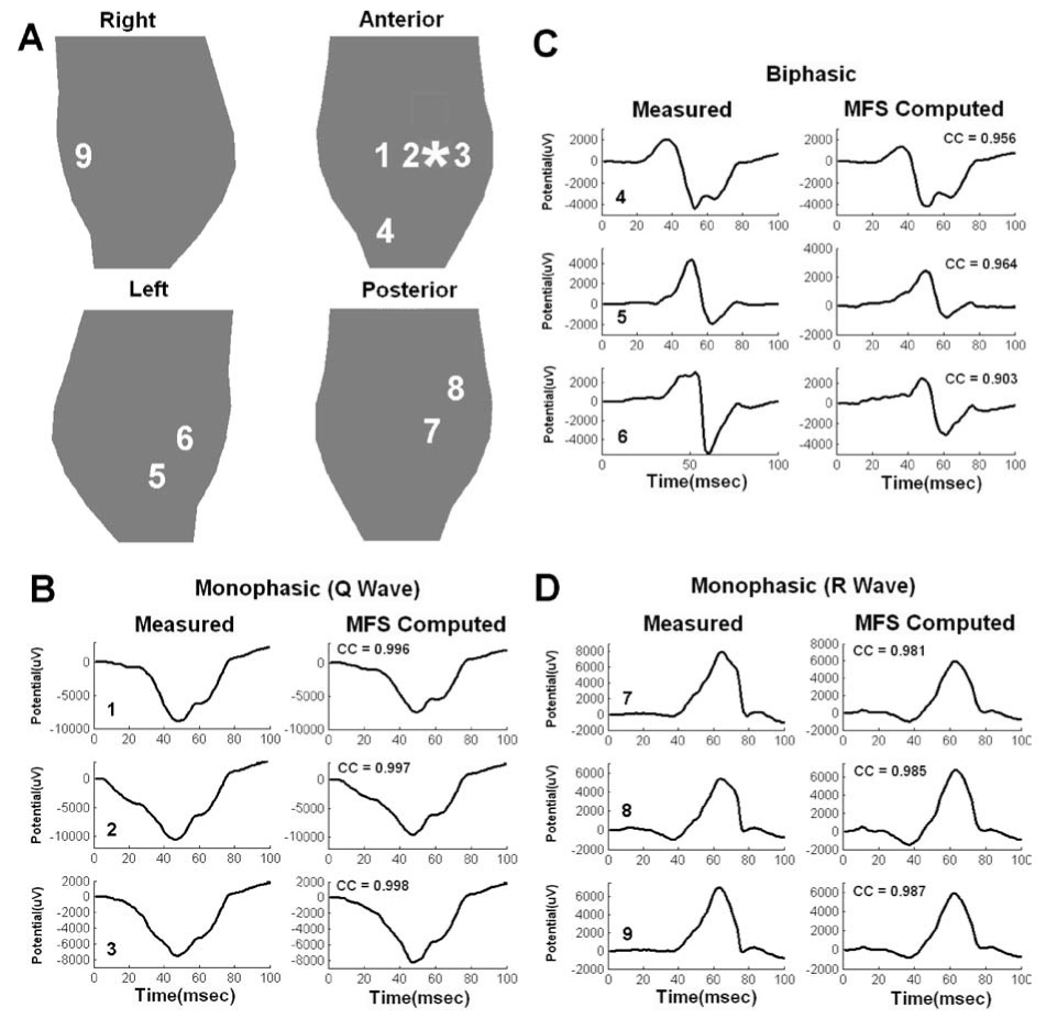
Canine epicardial electrograms (measured and computed using MFS ECGI) from selected locations on the heart surface for pacing from the same single site as in Fig. 2 (indicated by the asterisk). (A) Four views of epicardial surface. Numbers identify locations of the electrograms in the other panels. Measured (left column) and computed (right column) electrograms are compared in B, C and D. Number on the bottom left of each panel identifies the electrogram location (corresponding to numbers in A). (B) Monophasic (Q wave) electrograms from sites 1, 2 and 3. (C) Biphasic electrograms from sites 4, 5 and 6. (D) Monophasic (R wave) electrograms from sites 7, 8 and 9. CC is the Correlation Coefficient between invasive and noninvasive electrograms, indicating high level of similarity.
FIGURE 4.
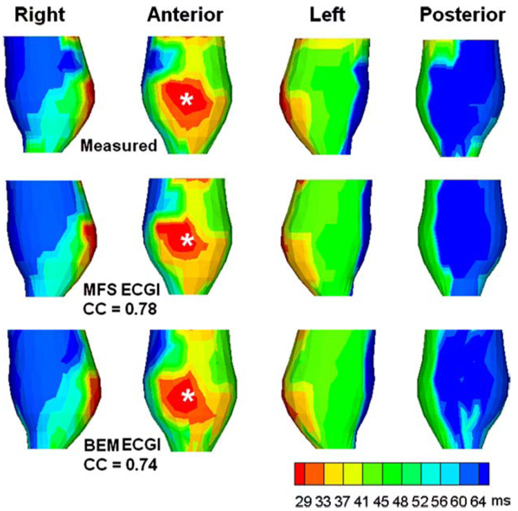
Canine epicardial isochrone map for pacing from the same single site as in Fig. 2 (indicated by the asterisk). Top row shows the directly measured isochrones (four views) displaying the anterior pacing site. Middle row shows the noninvasively reconstructed isochrone map computed using MFS ECGI. Bottom row shows the noninvasively reconstructed isochrone map computed using BEM ECGI.
RV Endocardial Pacing in a Human Subject
Figure 5 compares epicardial potential maps computed with BEM ECGI and MFS ECGI in a human subject during RV pacing (anterior view). There are 447 epicardial nodes, 115 torso nodes and 562 (447 + 115) virtual source points in this dataset. The pacing site as determined from CT images is marked by the white asterisk. Three reconstructions are compared: Left, BEM ECGI with an automatically generated mesh; Middle, MFS ECGI; Right, BEM ECGI with a manually optimized mesh. Panel A shows epicardial potential maps during activation, 62 ms after pacing. The negative region (dark blue) generated by unedited BEM ECGI is fragmented, due to meshing artifacts. The three negative regions could be interpreted erroneously as reflecting three pacing sites. MFS ECGI effectively avoids such fragmentation and reconstructs a quasi-elliptical negative region, reflecting the single pacing site. After manual mesh editing, fragmentation of the negative region is eliminated, demonstrating that the fragmentation is mesh related. Panel B of Fig. 5 shows a reconstructed epicardial potential map for the same protocol during repolarization (205 ms after pacing). As expected during pacing, the negative region of activation in panel A is replaced by a positive region (red).65,66 Similar to Panel A, fragmentation of the positive region is observed for unedited BEM ECGI, but not for MFS ECGI; it is eliminated from the BEM ECGI reconstruction after manual mesh editing.
FIGURE 5.
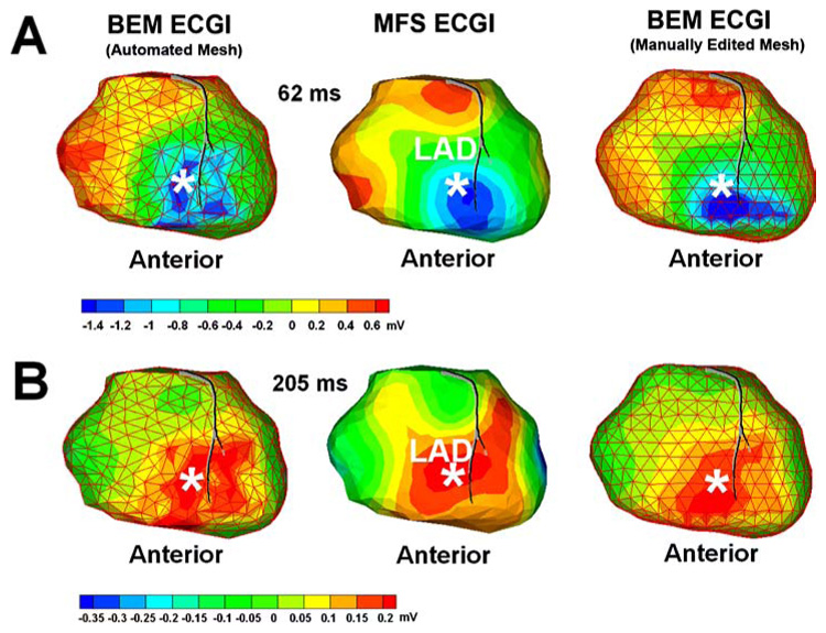
Panel A: Human epicardial potential map (anterior view) 62 ms after pacing from a single RV endocardial site (marked by the asterisk). Left: BEM ECGI reconstruction with initial mesh (non-optimized), showing fragmentation of the negative region (blue) caused by meshing artifact. Middle: MFS ECGI reconstructs a single continuous minimum (blue) associated with single-site pacing. Right: BEM ECGI reconstruction with manually-edited mesh, showing that fragmentation is mesh related. Panel B: Human epicardial potential map (anterior view) during repolarization for pacing from the same site (205 ms after pacing).
The error in locating the pacing site is 14 mm using BEM ECGI (by fitting an ellipse over the three negative regions in the automated mesh reconstruction), 8 mm using BEM ECGI with the manually optimized mesh, and 5 mm using MFS ECGI. In order to improve the unedited BEM ECGI reconstruction result, several manual iterations of mesh editing and optimization were required.
Simultaneous RV Endocardial and LV Epicardial Pacing
Figure 6 shows MFS ECGI reconstructions during simultaneous RV endocardial and LV epicardial pacing in a patient undergoing bi-ventricular pacing for CRT. There are 437 epicardial nodes, 189 torso nodes and 626 (437 + 189) virtual source points in this dataset. Panel A is an epicardial potential map 40 ms after pacing, displayed in three partially overlapping views. The asterisks mark the pacing sites locations determined from CT images. Panel B shows an epicardial isochrone map on the same views. From the isochrone map, it is determined that epicardial activation above the endocardial RV pacing site occurred 25 ms later than epicardial activation around the epicardial LV pacing site. Given that pacing from both leads was simultaneous, the delay probably reflects, at least in part, endocardial to epicardial wave front propagation in the RV ventricular wall.
FIGURE 6.
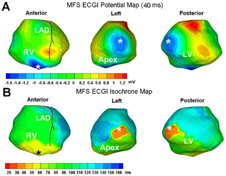
Human epicardial potential map and isochrone map for simultaneous RV and LV pacing (pacing sites marked by the asterisks *; note that the left and posterior views show the same pacing site). Panel A shows the MFS ECGI reconstructed potential map 40 ms after pacing (three partially overlapping views). Typical quasi-elliptic negative region (blue) surrounds each pacing site. Panel B shows the corresponding MFS ECGI reconstructed isochrone map in the same format.
From both isochrone maps and potential maps the RV pacing site and LV pacing site are located within 5.2 and 7.4 mm, respectively, of their locations as determined from CT. This accuracy is similar to the results of BEM ECGI after several iterations of mesh optimization.
Normal Human Atrial Activation
Figure 7 shows normal atrial activation isochrones reconstructed by MFS ECGI for a healthy volunteer. There are 322 atrial epicardial nodes, 228 torso nodes and 550 (322 + 228) virtual source points in this dataset. Earliest activation starts in the right atrium (RA) between the aorta and superior vena cava (SVC), near the anatomical location of the sinoatrial node (SA node). From the SA node, the impulse propagates radialy to the left atrium (LA) and the rest of the RA (the black arrows show the propagation pathway). The LA appendage (LAA) activates last. The atrial isochrones by MFS ECGI are practically identical to those reconstructed using BEM ECGI.2 Both reconstructions provide activation patterns that are very consistent with directly measured atrial isochrones in normal isolated human hearts.25
FIGURE 7.
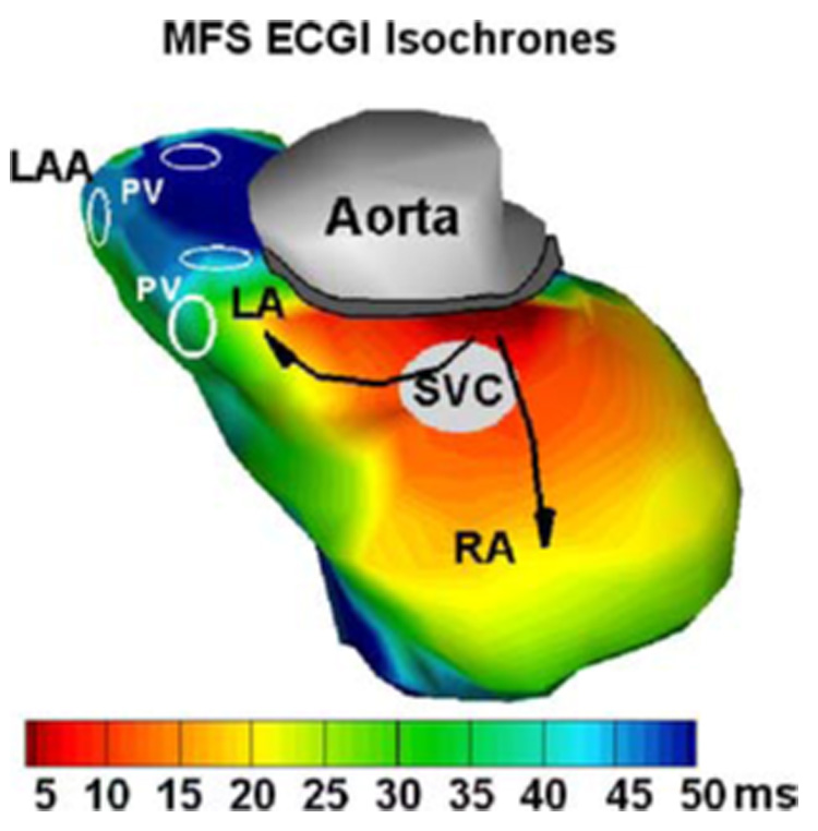
Normal human atrial activation isochrones reconstructed with MFS ECGI. RA: Right Atrium; LA: Left Atrium; LAA: Left Atrial Appendage; PV: Pulmonary Vein; SVC: Superior Vena Cava. Black arrows indicate direction of activation spread.
DISCUSSION
In this paper we implement a meshless method, MFS, for noninvasive ECGI and evaluate its accuracy and performance. ECGI is formulated in terms of potentials, computing potentials on the epicardial surface of the heart from electrocardiographic potentials measured on the body surface.3,29,71,80 The existence of a well-behaved, analytic fundamental solution for the Laplace operator in 3D42 makes MFS highly suitable for the ECGI application.
Being a potential-based scheme, ECGI reconstructs epicardial potentials, from which electrograms and activation sequences (isochrones) can also be computed. This approach is applicable not only during cardiac activation, but provides images of repolarization as well.32 A different approach to inverse electrocardiography has been to compute directly the activation sequences on both epicardial and endocardial surfaces of the heart.43,44,60 The potential-based approach has also been used to reconstruct potentials on the endocardial surface from a non-contact intracavitary catheter.8,48,51,52,81 It should be noted that while for the potential-based approach optimizing the mesh (a procedure requiring manual editing) is the time-limiting step, for the activation-based approach60 it is the inverse computation which utilizes a nonlinear-optimization iterative scheme, a complex time consuming process. Mesh related artifacts mainly affect patterns of epicardial potential maps and magnitudes of electrograms in the potential-based ECGI reconstruction. The morphology of electrograms (from which activation times are determined) and activation patterns (isochrones) are minimally affected by mesh structure. This suggests that the activation-time approach that only computes isochrones is less sensitive to mesh properties.
Geometry and Torso Inhomogeneities
The importance to inverse electrocardiography of geometry accuracy and of conductivity inhomogeneities in the torso volume conductor (due to the lungs and other torso compartments) has been evaluated extensively.20,45,46,71 Huiskamp and van Oosterom45 concluded that a tailored accurate geometry is required for accurate ECGI inverse computation. Other studies46,71 showed that although the accuracy of reconstruction depends on accurate knowledge of the geometry, small errors in geometry determination (e.g. 1-cm shift error in heart position) can be tolerated by ECGI without major deterioration of reconstruction quality. A study using realistic human anatomy69 demonstrated that a homogeneous model of the torso produced less accurate epicardial potential magnitudes than an inhomogeneous model, but epicardial potential patterns, electrogram morphologies, isochrones, and locations of pacing sites were reconstructed with comparable accuracy when the torso was assumed homogenous. Independence of epicardial patterns from torso volume-conductor properties was demonstrated experimentally as well.39 Based on results of these inhomogeneity studies, MFS ECGI is applied and tested here in a homogeneous torso volume-conductor. However, if needed the internal inhomogeneities can be included in BEM ECGI by extending the transfer matrix A to include the boundaries of internal torso compartments.68 Similar to BEM, the MFS approach can also be extended to a multi-compartment volume-conductor. Malik54 has shown how MFS can be applied to a multi-dielectric media problem. For such multi-compartment problem additional boundary conditions must be satisfied, namely continuity of potential and normal component of current at each inter-compartmental interface.64 Regional formulation of MFS for computation of electric fields was developed in the early 90’s.9,10 Recently a domain decomposition method was combined with MFS for solving the inhomogeneous multi-compartment problems.7 This approach can be applied to MFS ECGI in cases where the effect of torso inhomogeneities is of interest.
Mesh-Related Considerations
MFS application in ECGI offers a meshless alternative to boundary element (BEM) and finite element (FEM) methods27,75 that require meshing the heart and torso. Mesh quality is well known to affect both the time and accuracy of numerical solutions to PDE-based applications.4 A “bad” mesh structure that contains elements of non-uniform area, non-uniform angle or non-uniform aspect ratio, can introduce serious artifacts in the numerical computation. This is especially true for the ECGI application, because the ill-posed inverse computation76 that is involved tends to amplify such mesh related numerical errors (Fig. 5). Non-uniform mesh elements are difficult to avoid in meshing complex surfaces including the heart, especially in the presence of structural disease. Efficient methods for mesh optimization are the topic of ongoing research.4,13,30 For ECGI applications, it is difficult to define general criteria for automated optimal mesh generation because the mesh related artifacts are influenced by the ill-posed inverse computation. BEM ECGI usually requires several time-consuming manual iterations for mesh optimization (we use a constant potential field as a calibration dataset for this purpose). Even after an optimized mesh is constructed, BEM requires manipulation of the 3D surface mesh and computation of a complicated singular surface integral over each mesh element. Being a meshless method, MFS ECGI bypasses these procedures.
Figure 5 demonstrates that fragmentation of reconstructed epicardial potentials is mesh dependent. Several iterations of manual editing improved the mesh and removed fragmentation, resulting in a less fragmented and smoother reconstruction. However, mesh-related artifacts were still present after editing (Fig. 5, right panel), indicating that even several iterations did not result in an optimal mesh. Based on our experience, obtaining a fully optimized mesh that eliminates all artifacts is a very difficult and time consuming process. MFS ECGI does not require meshing and mesh optimization, avoiding this time consuming manual step that can introduce artifacts in the reconstructed images. It is possible that different regularization schemes8,14,34,40 than the ones employed here could provide better accuracy with an unedited mesh, or that better mesh generation algorithms optimized for ECGI could be developed. These possibilities remain to be investigated in future studies.
As shown in Eq. (3), normal vectors are required for the MFS computation. In the results shown here, normal vectors are constructed using the initial unedited mesh, which is generated very quickly by Amira (TGS Template Graphics Software, Inc.) without mesh editing. This may create the impression that MFS is not completely meshfree. The field of meshless approaches is progressing rapidly, including meshless methods for determining normal directions for given surfaces. For example, the Radial Basis Functions (RBF) method17,18 obtains the 3D surface representation and computes analytically the surface normal/tangent vectors without forming a mesh. Figure 8 compares MFS ECGI reconstructions (potential maps and electrograms) with mesh-generated normal vectors and with meshless normal vectors obtained using RBF. Panels A and B show the reconstructed potential maps during depolarization and repolarization, respectivcely. Panel C shows reconstructed electrograms from selected epicardial locations. Both methods produce very similar results. In addition, point-based rendering methods are also emerging very quickly,72 allowing for direct rendering of the surface without the creation of a polygonal mesh representation.
FIGURE 8.
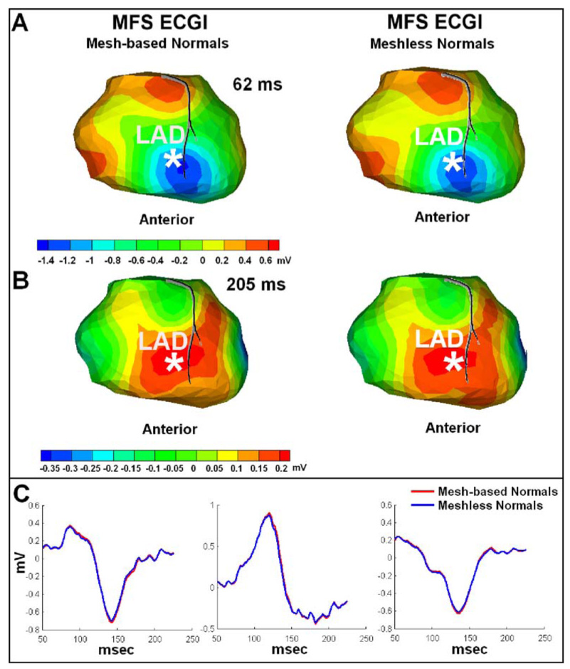
Comparison of MFS ECGI reconstructions with mesh-based and meshless normal vectors. Panel A: Human epicardial potential map (anterior view) 62 ms after pacing from a single RV endocardial site (marked by the asterisk). Left: MFS ECGI reconstruction with normal vectors computed using a mesh. Right: MFS ECGI reconstruction with normal vectors computed without a mesh, using Radial Basis Function (RBF). Panel B: Human epicardial potential map (anterior view) during repolarization for pacing from the same site (205 ms after pacing). Same format as Panel A. Panel C: Human epicardial electrograms from selected locations on the heart surface for the same pacing dataset. Red traces show the MFS ECGI reconstruction with mesh-based normal vectors. Blue traces show the MFS ECGI reconstruction with meshless normal vectors computed using RBF.
Morphing a template mesh of a stylized heart could be an effective approach for creating a patient-specific mesh in BEM ECGI. However, it requires evaluation in this context. One of the major concerns regarding application of morphing is that many hearts that can benefit from clinical ECGI have pathologies that modify greatly the heart geometry (e.g. dilation, presence of diverticuli or anneurisms). Such localized structural deformations cause large deviations from the anatomy of a template heart. Our laboratory uses Amira to obtain the initial surface mesh for such diseased hearts. The initial mesh requires manual editing to obtain an improved mesh structure for reduction of mesh-related artifacts.
For a given problem, the condition number of the  matrix in MFS is usually larger than that of the forward matrix in BEM. For the torso-tank data in this study, the condition number is 2.3516e + 014 for BEM, and 9.1934e + 016 for MFS; however better accuracy is obtained with MFS. Several studies by others11,37,38 have suggested that the numerical accuracy of MFS is only minimally affected by the condition properties of the matrix. Recent work by Christiansen and Saranen23 and Christiansen and Hansen22 also suggests that the condition number as commonly defined is not an appropriate measure of numerical stability. Better accuracy with a larger condition number was also obtained when a second order BEM scheme was applied in ECGI reconstruction.35
A possible advantage of BEM ECGI is that the torso geometry can be constructed with greater precision than that delineated by the electrodes. Consequently, the transfer matrix can be computed with greater accuracy. Such augmentation can not be implemented in MFS ECGI. However, since the zero Neumann condition (no current flow across the torso-air boundary) is valid on the entire torso surface, Neumann conditions at more torso locations (Eq. (3)) can be added in the MFS ECGI formulation (Eq. (4)). We examined the benefit of doing so and results (not shown) show similar or only slightly improved electrograms and potential maps as judged by CC and RE values.
Placement of Virtual Source Points
Implementation of MFS requires choosing a fictitious boundary for placing the virtual source points. There are two widely used approaches for doing so, the dynamic and static methods.37 In the dynamic configuration, the fictitious boundary is determined together with the solution50 via a complex, time-consuming nonlinear optimization procedure which does not always guarantee global convergence. In the static configuration, the fictitious boundary is pre-selected corresponding to the real boundary based on some fixed (static) rules (criteria), for example the inflation-deflation rule used here. For different patients’ geometries, the corresponding fictitious boundaries that are generated by the static rule are different. The static method is not the optimal implementation of MFS, but it is very easy to implement and highly suitable for practical engineering applications. Very good accuracy has been obtained using the static method in engineering and industrial applications of MFS,41 including the application presented here. Optimal placement of the virtual source points poses a difficulty for MFS implementation. However, much faster and more efficient nonlinear optimization schemes28 are under development, which could facilitate use of the dynamic method in MFS ECGI.
The “inflation-deflation” procedure used in our reconstructions was designed and tested using data from the human-shaped torso-tank experiments,62 where directly measured epicardial potentials provided a gold standard for evaluation. Because the heart surface is globally convex, the “inflation-deflation” procedure works well for most heart geometries. In the presence of structural heart disease, the heart surface could contain concave regions. For such geometry, static inflation or deflation relative to a fixed point may place some fictitious points in the domain of interest. In these cases, special care is needed to insure that all fictitious points lie outside the domain of interest. An alternative approach is to employ a more general “inflation-deflation” procedure, which does not inflate or deflate the boundary relative to a fixed point and insures that the virtual source points are placed outside the domain of interest. For example, in the FastRBF toolbox,17,18 inflation and deflation are achieved by computing isosurfaces based on the distance from the actual boundary, which insures that the fictitious nodes are placed outside the domain for all types of heart geometry. This method is demonstrated in panel A of Fig. 9 for the complex geometry of the atria in Fig. 7. A 3D Radial Basis Function (RBF)17,18 computes a signed distance from the actual object’s surface. If the normal direction is inward, points inside the object have positive distances (red) while points outside have negative distances (green-blue). The object’s surface is defined as the zero set of the function (yellow). In Panel A, the RBF function grid values are shown on three orthogonal planes: x=60 (mm), y=90 (mm), and z=30 (mm). By setting different RBF values, different inflated (or deflated) surfaces of the atria can be obtained. Panel B of Fig. 9 shows an inflated atria surface obtained by selecting RBF=5(mm). This figure demonstrates that this more general procedure can be used for complex heart geometry such as the atria in this example, or ventricles with irregular geometry due to disease (e.g. diverticuli or aneurisms).
FIGURE 9.
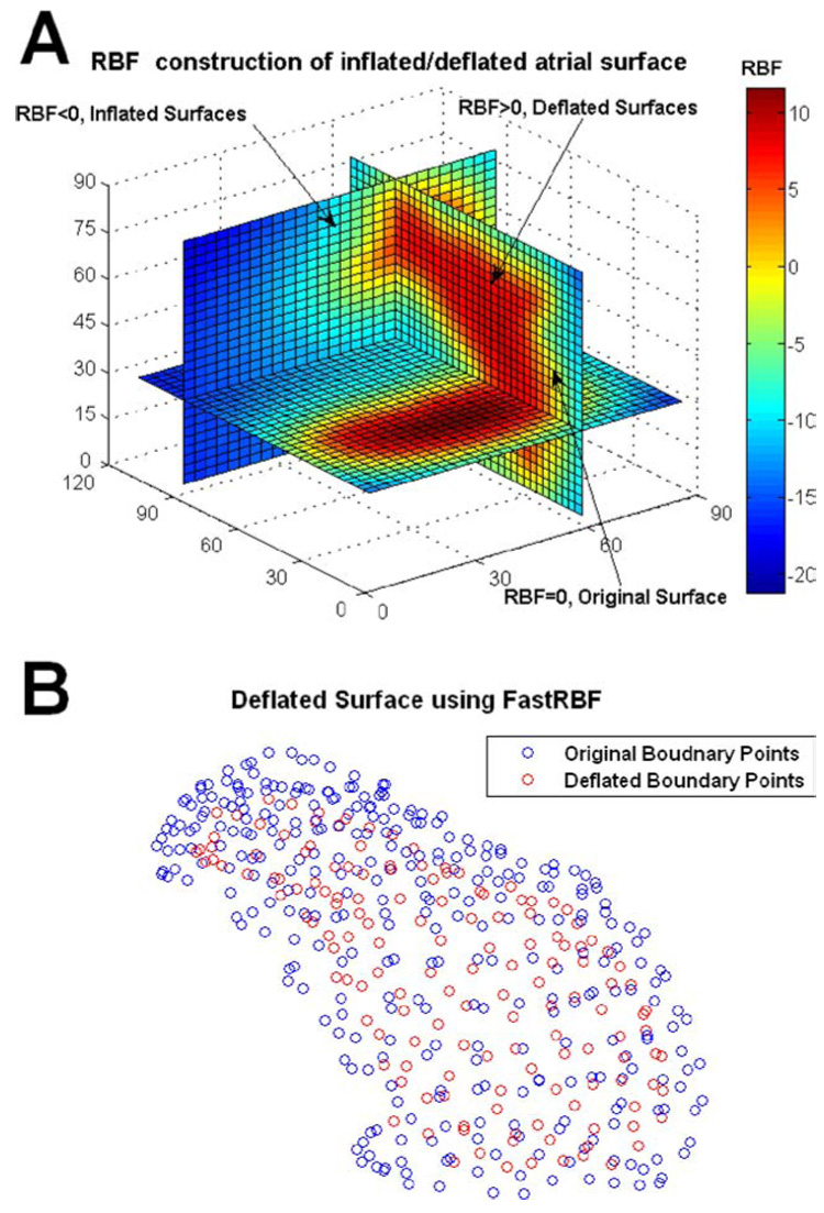
Panel A: Radial Basis Function (RBF) representation of the atrial surface in Fig. 7 and corresponding inflated/deflated surfaces. The RBF function grid values are shown on three orthogonal planes: x=60 (mm), y=90 (mm), and z=30 (mm). The original boundary is represented by the isosurface with RBF=0(mm). Since the positive normal direction is chosen inward, deflated surfaces are represented by isosurfaces with RBF>0 and inflated surfaces by the isosurfaces with RBF<0. Panel B: A deflated atrial surface obtained by selecting RBF=5 (mm). Blue circles represent the original boundary points, and red circles represent the deflated surface points; all red circles are enclosed by the 3D surface defined by the blue circles.
Determination of the optimal position of the fictitious nodes relative to the actual boundary is a difficult problem that is the subject of ongoing research.37 For noise-free boundary conditions, Golberg and Chen37 have shown that the accuracy of MFS improves when the fictitious nodes are moved far away from the actual boundary. However, for noisy boundary conditions that always exist in actual engineering applications, Mera55 has found that accuracy deteriorates when the fictitious points are placed too close or too far from the actual boundary. If the fictitious points (singularities) are placed too close to the actual boundary, MFS will have to evaluate nearly-singular matrix elements during formation of the matrix  (Eq. (4)). If the fictitious points are placed too far from the actual boundary, the rows in the top half of matrix  become very similar to each other, as do the rows in the bottom half; this increases the singularity of the matrix. We used several datasets from the human-shaped torso-tank experiments,62 to evaluate the dependence of accuracy on the positions of fictitious nodes. The most accurate reconstructions were obtained for deflating by a factor in the range 0.6 to 0.9 and inflating by a factor in the range 1.1–1.5 (within these ranges, accuracy did not depend significantly on the exact parameter value). Based on this empirical observation in a realistic human-shaped heart-torso geometry, we chose 0.8 as the deflating parameter and 1.2 as the inflating parameter for all studies presented here.
With this simple “inflation-deflation” scheme, the number of fictitious points is chosen based on practical considerations to be equal to the number of actual boundary nodes. This is a simple choice employed in this paper, and is not a requirement of the MFS method. Mera55 has shown that the accuracy of inverse computation using MFS for a backward heat conduction problem improved with increasing number of fictitious nodes. He also found that the accuracy did not improve once the number of fictitious nodes exceeded a certain limit. Since very good reconstruction accuracy was obtained here with the number of fictitious nodes set equal to the number of boundary nodes, we did not attempt to increase this number. It is possible that the number of fictitious nodes could be reduced without significant loss of accuracy as suggested by Mera.55 Systematic evaluation is needed to determine the optimal number of fictitious points in the context of ECGI.
ACKNOWLEDGMENTS
We thank Professor C.S. Chen from University of Southern Mississippi for very useful advice regarding MFS theory and implementation. We thank Dr. Bruno Taccardi for the torso-tank experiments, conducted in his laboratory at the University of Utah. We would also like to acknowledge the assistance of L. Ciancibello in acquiring and transferring the CT imaging data and K. Ryu for his assistance in body surface potential mapping. Special thanks go to Dr. Ping Jia for helpful discussions. This study was supported by NIH-NHLBI Merit Award R37-HL-33343 and Grant R01-HL-49054 (to Yoram Rudy) and by a Whitaker Foundation Development Award. Yoram Rudy is the Fred Saigh distinguished professor at Washington University in St Louis. We appreciate the extensive reviews provided by the manuscript reviewers; they helped making this a better paper.
APPENDIX: FORMULATION OF MFS FOR LAPLACIAN OPERATOR
MFS has evolved from traditional boundary integral methods. Without forming a mesh, MFS uses a set of points to solve numerically partial differential equations. Details of this method can be found in the review article.37 The following Dirichlet boundary value problem is used to describe the theoretical formulation of MFS for the Laplacian operator:
| (a1) |
| (a2) |
where ▽² is the Laplace differential operator with a known fundamental solution f (r) in 3D space. u(x) is a potential function in a source-free domain Ω and b(x) is the Dirichlet boundary condition. According to the definition of fundamental solution,27 the fundamental solution of the Laplace operator can be obtained by solving the following equation for f(r):
| (a3) |
where δ(r) is the delta function, r = ‖x − y‖ is the 3D Euclidean distance between point x and point y, x, y ∈ Ω. f (r) in two dimensions (2D) and three dimensions (3D) is:53
| (a4) |
Both BEM and MFS use the same Green’s function in 3D space. However BEM integrates this function locally over elements of the real surface and requires computation of complex singular integrals. By placing the fictitious source points outside the domain of interest, MFS employs global integration and avoids the need to compute complex singular integrals.
The traditional boundary integral approach is to represent the solution u(x) in term of a double layer potential:36,63
| (a5) |
where, n is the outward pointing normal at point y, e(y) is an unknown density function. Equivalently a single layer potential representation of u(x) can be used19,36
| (a6) |
The source density distribution e(y) can be determined by solving the following equation under the assumption of a double layer:
| (a7) |
or under the assumption of a single layer:
| (a8) |
However, singular integrals are involved in both cases. To alleviate this difficulty, the following formulation, similar to the single layer potential in (a6), has been used:50
| (a9) |
where the auxiliary boundary Γ̂ is the surface of the auxiliary domain Ω̂ containing the domain Ω (Fig. 1).
Two different approaches for selecting Γ̂ and its fictitious source points y are described in the literature:36 static configuration and dynamic configuration. In static configuration, the fictitious boundaries are fixed and pre-selected. The method is easy to implement and use in practical applications. For dynamic configuration, the location of fictitious boundaries is determined together with the solution50 by a complex, time-consuming nonlinear optimization procedure, which greatly limits its practical application. Since the geometry of the 3D domain between the torso surface and the heart surface is similar for all humans, the static approach is the method of choice for ECGI application.
Because f (‖x − y‖) is the fundamental solution of the Laplace operator [Eq. (a3)], (a9) satisfies the differential Eq. (a1). Therefore we need only to apply the boundary condition (a2):
| (a10) |
where the source density distribution e(y), y ∈ Γ̂, is to be determined. Once the source density is determined, Eq. (a1) subject to (a2) is solved. The analytic integral representation of (a10) implies that there is an infinite number of source density points on Γ̂. In order to apply numerical methods to the solution, it is necessary to discretize e(y). Assume ψi(y)i= 1, 2 … ∞ is a complete set of functions on Γ̂, e(y) can be approximated by:
| (a11) |
Substituting (a11) into (a10) and satisfying the boundary conditions at the N boundary points xk ∈ Γ, k = 1, 2, …N; we have
| (a12) |
Since the fictitious boundary Γ̂ is located outside the physical domain (Fig. 1), the integrand f (‖xk − y‖) is nonsingular and standard quadrature rules can be applied giving
| (a13) |
where wj is a weight factor and M is the number of fictitious nodes on the fictitious boundary Γ̂.37
From (a12) and (a13), we obtain:
| (a14) |
Then:
| (a15) |
where:
| (a16) |
For completeness,11 a constant a0 is added to (a15):
| (a17) |
After Eq. (a17) is solved for a0 and aj(j = 1, 2, …, M), the solution to (a1) can be approximated by:
| (a18) |
The approximate solution ua to Eq. (a1) is represented by a linear combination of fundamental solutions of the governing equation with the singularities yj, j = 1, 2, …, M, placed outside the domain of the problem.
MFS is applicable not only to the above boundary value problem, but also to the Cauchy problem42 that underlies ECGI. In this problem, both Dirichlet and Neumann boundary conditions are given only on portion of the boundary:42
| (a1) |
| (a19) |
| (a20) |
For the Neumann condition (a20), the gradient at point x is along the outward normal to the boundary at that point. Similar to Eq. (a17), MFS can be used to discretize the Dirichlet and Neumann boundary conditions (Eq. (a19) and Eq. (a20)) as follows:
| (a21) |
| (a22) |
After solving for the coefficients (a0, aj, j = 1, 2, …, M), subject to the boundary conditions (a19) and (a20), the solution to (a1) can be approximated using Eq. (a18).
Convergence analysis of MFS for Laplace’s equation was conducted by Cheng.21 When the problem boundary and boundary conditions are smooth functions, MFS converges exponentially to the solution of the problem. This analysis was conducted for 2D; Golberg and Chen36 provided arguments that similar convergence properties exist in 3D.
References
- 1.Atkinson KE, Chien D. Piecewise Polynomial collocation for boundary integral equations. SIAM J. Sci. Stat. Comput. 1995;16:651–681. [Google Scholar]
- 2.Barr RC, Spach MS. Inverse calculation of QRS-T epicardial potentials from body surface potential distributions for normal and ectopic beats in the intact dog. Circ. Res. 1978;42(5):661–675. doi: 10.1161/01.res.42.5.661. [DOI] [PubMed] [Google Scholar]
- 3.Barr RC, Spach MS. Inverse solutions directly in terms of potentials. In: Nelson CV, Geselowitz DB, editors. The Theoretical Basis of Electrocardiography. Oxford: Clarendon Press; 1976. pp. 294–304. [Google Scholar]
- 4.Batdorf M, Freitag LA, Ollivier-Gooch C. Computational study of the effect of unstructured mesh quality on solution efficiency; Proc. 13th AIAA Computational Fluid Dynamics Conf.: 1888; 1997. [Google Scholar]
- 5.Beer G, Watson JO. Introduction to Finite and Boundary Element Methods for Engineers. West Sussex: Wiley; 1992. [Google Scholar]
- 6.Belytschko T, Krongauz Y, Organ D, Fleming M, Krysl P. Meshless methods: An overview and recent developments. Comput. Method. Appl. Mech. Eng. 1996;139:3–47. [Google Scholar]
- 7.Berger JR, Karageorghis A. The method of fundamental solutions for heat conduction in layered materials. Int. J. Numer. Methods Eng. 1999;45(11):1681–1694. [Google Scholar]
- 8.Berrier KL, Sorensen DC, Khoury DS. Solving the inverse problem of electrocardiography using a Duncan and Horn formulation of the Kalman filter. IEEE Trans. Biomed. Eng. 2004;51(3):507–515. doi: 10.1109/TBME.2003.821027. [DOI] [PubMed] [Google Scholar]
- 9.Blaszczyk A. Formulations based on region-oriented charge simulation for electromagnetics. IEEE Trans. Magn. 2000;36(4):701–704. [Google Scholar]
- 10.Blaszczyk A, Steinbigler H. Region-oriented charge simulation. IEEE Trans. Magn. 1994;30(5):2924–2927. [Google Scholar]
- 11.Bogomolny A. Fundamental solutions method for elliptic boundary value problems. SIAM J. Numer. Anal. 1985;22:644–669. [Google Scholar]
- 12.Brebbia CA, Telles JCF, Wrobel LC. Boundary Element Techniques: Theory and Applications in Engineering. Berlin, Germany: Springer Verlag; 1984. [Google Scholar]
- 13.Brewer M, Diachin L, Leurent T, Melander D. The mesquite mesh quality improvement toolkit; Proceedings, 12th International Meshing Roundtable; 2003. pp. 239–250. [Google Scholar]
- 14.Brooks DH, Ahmad GF, MacLeod RS, Maratos GM. Inverse electrocardiography by simultaneous imposition of multiple constraints. IEEE Trans. Biomed. Eng. 1999;46(1):3–18. doi: 10.1109/10.736746. [DOI] [PubMed] [Google Scholar]
- 15.Burnes JE, Taccardi B, Ershler PR, Rudy Y. Noninvasive electrocardiogram imaging of substrate and intramural ventricular tachycardia in infarcted hearts. J. Am. Coll. Cardiol. 2001;38(7):2071–2078. doi: 10.1016/s0735-1097(01)01653-9. [DOI] [PMC free article] [PubMed] [Google Scholar]
- 16.Burnes JE, Taccardi B, Rudy Y. A noninvasive imaging modality for cardiac arrhythmias. Circulation. 2000;102(17):2152–2158. doi: 10.1161/01.cir.102.17.2152. [DOI] [PMC free article] [PubMed] [Google Scholar]
- 17.Carr JC, Beatson RK, Cherrie JB, Mitchell TJ, Fright WR, McCallum BC, Evans TR. Reconstruction and representation of 3D objects with radial basis functions; Proceedings of the 28th Annual Conference on Computer Graphics and Interactive Techniques; 2001. pp. 67–76. [Google Scholar]
- 18.Carr JC, Fright WR, Beatson RK. Surface interpolation with radial basis functions for medical imaging. IEEE Trans. Med. Imaging. 1997;16(1):96–107. doi: 10.1109/42.552059. [DOI] [PubMed] [Google Scholar]
- 19.Chen Y, Atkinson K. Solving a single layer integral equation on surface in R3. SIAM J. Num. Anal., Reports on Computational Mathematics #51. 1994 [Google Scholar]
- 20.Cheng LK, Bodley JM, Pullan AJ. Effects of experimental and modeling errors on electrocardiographic inverse formulations. IEEE Trans. Biomed. Eng. 2003;50(1):23–32. doi: 10.1109/TBME.2002.807325. [DOI] [PubMed] [Google Scholar]
- 21.Cheng RSC. Deta-Trigonometric and Spline Methods using the Single-Layer Potential Representation. Ph.D. dissertation. University of Maryland; 1987. [Google Scholar]
- 22.Christiansen S, Hansen PC. The effective condition number applied to error analysis of certain boundary collocation methods. J. Comput. Appl. Math. 1994;54:15–36. [Google Scholar]
- 23.Christiansen S, Saranen J. The conditioning of some numerical methods for first kind integral equations. J. Comput. Appl. Math. 1996;67:43–58. [Google Scholar]
- 24.Colli-Franzone P, Guerri L, Tentoni S, Viganotti C, Baruffi S, Spaggiari S, Taccardi B. A mathematical procedure for solving the inverse problem of electrocardiography. Math. Biosci. 1985;77:353–396. [Google Scholar]
- 25.Durrer D, van Dam RT, Freud GE, Janse MJ, Meijler FL, Arzbaecher RC. Total excitation of the isolated human heart. Circulation. 1970;41(6):899–912. doi: 10.1161/01.cir.41.6.899. [DOI] [PubMed] [Google Scholar]
- 26.Fairweather G, Karageorghis A, Martin PA. The method of fundamental solutions for scattering and radiation problems. Engineering Analysis with Boundary Elements. 2003;27(7):759–769. [Google Scholar]
- 27.Fairweather G, Karageorghis A. The method of fundamental solutions for elliptic boundary value problems. Adv. Comput. Math. 1998;9:69–95. [Google Scholar]
- 28.Fischer G, Pfeifer B, Seger M, Hintermuller C, Hanser F, Modre R, Tilg B, Trieb T, Kremser C, Roithinger FX, Hintringer F. Computationally efficient noninvasive cardiac activation time imaging. Methods Inf. Med. 2005;44(5):674–686. [PubMed] [Google Scholar]
- 29.Franzone P, Taccardi B, Viganotti C. An approach to inverse calculation of epicardial potentials from body surface maps. Adv. Cardiol. 1978;21:50–54. doi: 10.1159/000400421. [DOI] [PubMed] [Google Scholar]
- 30.Freitag L, Leurent T, Knupp P, Melander D. MESQUITE design: Issues in the development of a mesh quality improvement toolkit; Proceedings of the 8th Intl. Conference on Numerical Grid Generation in Computational Field Simulations; 2002. pp. 159–168. [Google Scholar]
- 31.Gelernter HL, Swihart JC. A Mathematical-Physical Model of the Genesis of the Electrocardiogram. Biophys. J. 1964;17:285–301. doi: 10.1016/s0006-3495(64)86783-7. [DOI] [PMC free article] [PubMed] [Google Scholar]
- 32.Ghanem RN, Burnes JE, Waldo AL, Rudy Y. Imaging dispersion of myocardial repolarization, II: noninvasive reconstruction of epicardial measures. Circulation. 2001;104(11):1306–1312. doi: 10.1161/hc3601.094277. [DOI] [PubMed] [Google Scholar]
- 33.Ghanem RN, Jia P, Ramanathan C, Ryu K, Markowitz A, Rudy Y. Noninvasive electrocardiographic imaging (ECGI): comparison to intraoperative mapping in patients. Heart Rhythm. 2005;2(4):339–354. doi: 10.1016/j.hrthm.2004.12.022. [DOI] [PMC free article] [PubMed] [Google Scholar]
- 34.Ghodrati A, Brooks DH, Tadmor G, Punske B, MacLeod RS. Wavefront-based inverse electrocardiography using an evolving curve state vector and phenomenological propagation and potential models. Int. J. Bioelectromagn. 2005;7(2):210–213. [Google Scholar]
- 35.Ghosh S, Rudy Y. Accuracy of quadratic versus linear interpolation in noninvasive Electrocardiographic Imaging (ECGI) Ann. Biomed. Eng. 2005;33(9):1187–1201. doi: 10.1007/s10439-005-5537-x. [DOI] [PMC free article] [PubMed] [Google Scholar]
- 36.Golberg MA, Chen CS. Discrete Projection Methods for Integral Equations. Southampton: Computational Mechanics Publications; 1996. [Google Scholar]
- 37.Golberg MA, Chen CS. The method of fundamental solutions for potential, Helmholtz and diffusion problems. In: Golberg MA, editor. Boundary Integral Methods - Numerical and Mathematical Aspects. Southampton-Boston: Computational Mechanics Publications; 1998. pp. 103–176. [Google Scholar]
- 38.Golberg MA, Chen CS, Karur SR. Improved multi-quadric approximation for partial differential equations. Engin. Anal. Bound. Elem. 1996;18:9–17. [Google Scholar]
- 39.Green LS, Taccardi B, Ershler PR, Lux RL. Epicardial potential mapping. Effects of conducting media on isopotential and isochrone distributions. Circulation. 1991;84(6):2513–2521. doi: 10.1161/01.cir.84.6.2513. [DOI] [PubMed] [Google Scholar]
- 40.Greensite F. The temporal prior in bioelectromagnetic source imaging problems. IEEE Trans. Biomed. Eng. 2003;50(10):1152–1159. doi: 10.1109/TBME.2003.817632. [DOI] [PubMed] [Google Scholar]
- 41.Hon YC, Wei T. A fundamental solution method for inverse heat conduction problem. Eng. Anal. Bound. Elem. 2004;28:489–495. [Google Scholar]
- 42.Hon YC, Wei T. Solving Cauchy problems of elliptic equations by the method of fundamental solutions. In: Kassab A, Brebbia CA, Divo E, Poljak D, editors. Boundary Elements XXVII. Southampton-Boston: WIT Press; 2005. pp. 57–65. [Google Scholar]
- 43.Huiskamp G, Greensite F. A new method for myocardial activation imaging. IEEE Trans. Biomed. Eng. 1997;44(6):433–446. doi: 10.1109/10.581930. [DOI] [PubMed] [Google Scholar]
- 44.Huiskamp G, van Oosterom A. The depolarization sequence of the human heart surface computed from measured body surface potentials. IEEE Trans. Biomed. Eng. 1988;35(12):1047–1058. doi: 10.1109/10.8689. [DOI] [PubMed] [Google Scholar]
- 45.Huiskamp G, van Oosterom A. Tailored versus realistic geometry in the inverse problem of electrocardiography. IEEE Trans. Biomed. Eng. 1989;36(8):827–835. doi: 10.1109/10.30808. [DOI] [PubMed] [Google Scholar]
- 46.Huiskamp GJ, van Oosterom A. Heart position and orientation in forward and inverse electrocardiography. Med. Biol. Eng. Comput. 1992;30(6):613–620. doi: 10.1007/BF02446793. [DOI] [PubMed] [Google Scholar]
- 47.Intini A, Goldstein RN, Jia P, Ramanathan C, Ryu K, Giannattasio B, Gilkeson R, Stambler BS, Brugada P, Stevenson WG, Rudy Y, Waldo AL. Electrocardiographic imaging (ECGI), a novel diagnostic modality used for mapping of focal left ventricular tachycardia in a young athlete. Heart Rhythm. 2005;2(11):1250–1252. doi: 10.1016/j.hrthm.2005.08.019. [DOI] [PMC free article] [PubMed] [Google Scholar]
- 48.Jia P, Punske B, Taccardi B, Rudy Y. Electrophysiologic endocardial mapping from a noncontact nonexpendable catheter: a validation study of a geometry-based concept. J. Cardiovasc. Electrophysiol. 2000;11(11):1238–1251. doi: 10.1046/j.1540-8167.2000.01238.x. [DOI] [PubMed] [Google Scholar]
- 49.Jia P, Ramanathan C, Ghanem RN, Ryu K, Varma N, Rudy Y. Electrocardiographic imaging of cardiac resynchronization therapy in heart failure: Observation of variable electrophysiologic responses. Heart Rhythm. 2006;3(3):296–310. doi: 10.1016/j.hrthm.2005.11.025. [DOI] [PMC free article] [PubMed] [Google Scholar]
- 50.Karageorghis A, Fairweather G. The method of fundamental solutions for the numerical solution of the biharmonic equation. J. Comput. Phys. 1987;69:435–459. [Google Scholar]
- 51.Khoury DS, Berrier KL, Badruddin SM, Zoghbi WA. Three-dimensional electrophysiological imaging of the intact canine left ventricle using a noncontact multielectrode cavitary probe: study of sinus, paced, and spontaneous premature beats. Circulation. 1998;97(4):399–409. doi: 10.1161/01.cir.97.4.399. [DOI] [PubMed] [Google Scholar]
- 52.Khoury DS, Taccardi B, Lux RL, Ershler PR, Rudy Y. Reconstruction of endocardial potentials and activation sequences from intracavitary probe measurements. Localization of pacing sites and effects of myocardial structure. Circulation. 1995;91(3):845–863. doi: 10.1161/01.cir.91.3.845. [DOI] [PubMed] [Google Scholar]
- 53.Kythe PK. Fundamental Solutions for Differential Operators and Applications. Boston-Basel-Berlin: Birkhauser; 1996. [Google Scholar]
- 54.Malik NH. A review of the charge simulation method and its applications. IEEE Trans. Electr. Insul. 1989;24(1):3–20. [Google Scholar]
- 55.Mera NS. The method of fundamental solutions for the backward heat conduction problem. Inverse Probl. Sci. Eng. 2005;13(1):65–78. [Google Scholar]
- 56.Messinger-Rapport BJ, Rudy Y. Noninvasive recovery of epicardial potentials in a realistic heart-torso geometry. Normal sinus rhythm. Circ Res. 1990;66(4):1023–1039. doi: 10.1161/01.res.66.4.1023. [DOI] [PubMed] [Google Scholar]
- 57.Messnarz B, Tilg B, Modre R, Fischer G, Hanser F. A new spatiotemporal regularization approach for reconstruction of cardiac transmembrane potential patterns. IEEE Trans. Biomed. Eng. 2004;51(2):273–281. doi: 10.1109/TBME.2003.820394. [DOI] [PubMed] [Google Scholar]
- 58.Modre R, Tilg B, Fischer G, Hanser F, Messnarz B, Seger M, Hintringer F, Roithinger FX. Ventricular surface activation time imaging from electrocardiogram mapping data. Med. Biol. Eng. Comput. 2004;42(2):146–150. doi: 10.1007/BF02344624. [DOI] [PubMed] [Google Scholar]
- 59.Modre R, Tilg B, Fischer G, Hanser F, Messnarz B, Seger M, Schocke MF, Berger T, Hintringer F, Roithinger FX. Atrial noninvasive activation mapping of paced rhythm data. J. Cardiovasc. Electrophysiol. 2003;14(7):712–719. doi: 10.1046/j.1540-8167.2003.02558.x. [DOI] [PubMed] [Google Scholar]
- 60.Modre R, Tilg B, Fischer G, Wach P. Noninvasive myocardial activation time imaging: a novel inverse algorithm applied to clinical ECG mapping data. IEEE Trans. Biomed. Eng. 2002;49(10):1153–1161. doi: 10.1109/TBME.2002.803519. [DOI] [PubMed] [Google Scholar]
- 61.Oster HS, Taccardi B, Lux RL, Ershler PR, Rudy Y. Electrocardiographic imaging: Noninvasive characterization of intramural myocardial activation from inverse-reconstructed epicardial potentials and electrograms. Circulation. 1998;97(15):1496–1507. doi: 10.1161/01.cir.97.15.1496. [DOI] [PubMed] [Google Scholar]
- 62.Oster HS, Taccardi B, Lux RL, Ershler PR, Rudy Y. Noninvasive electrocardiographic imaging: reconstruction of epicardial potentials, electrograms, and isochrones and localization of single and multiple electrocardiac events. Circulation. 1997;96:1012–1024. doi: 10.1161/01.cir.96.3.1012. [DOI] [PubMed] [Google Scholar]
- 63.Patridge PW, Brebbia CA, Wrobel LC. The Dual Reciprocity Boundary Element Method. Southampton-Boston: Computational Mechanics Publications; 1992. [Google Scholar]
- 64.Plonsey R, Barr RC. Bioelectricity: a Quantitative Approach. New York: Plenum Press; 1988. [Google Scholar]
- 65.Ramanathan C, Ghanem RN, Jia P, Ryu K, Rudy Y. Noninvasive electrocardiographic imaging for cardiac electrophysiology and arrhythmia. Nat. Med. 2004;10(4):422–428. doi: 10.1038/nm1011. [DOI] [PMC free article] [PubMed] [Google Scholar]
- 66.Ramanathan C, Jia P, Ghanem R, Calvetti D, Rudy Y. Noninvasive electrocardiographic imaging (ECGI): application of the generalized minimal residual (GMRes) method. Ann. Biomed. Eng. 2003;31(8):981–994. doi: 10.1114/1.1588655. [DOI] [PMC free article] [PubMed] [Google Scholar]
- 67.Ramanathan C, Jia P, Ghanem RN, Ryu K, Rudy Y. Activation and repolarization of the normal human heart under complete physiological conditions. Proc. Natl. Acad. Sci., U.S.A. (PNAS) 2006;103(16):6309–6314. doi: 10.1073/pnas.0601533103. [DOI] [PMC free article] [PubMed] [Google Scholar]
- 68.Ramanathan C, Rudy Y. Electrocardiographic imaging: I. Effect of torso inhomogeneities on body surface electrocardiographic potentials. J. Cardiovasc. Electrophysiol. 2001;12(2):229–240. doi: 10.1046/j.1540-8167.2001.00229.x. [DOI] [PubMed] [Google Scholar]
- 69.Ramanathan C, Rudy Y. Electrocardiographic imaging: II. Effect of torso inhomogeneities on noninvasive reconstruction of epicardial potentials, electrograms, and isochrones. J. Cardiovasc. Electrophysiol. 2001;12(2):241–252. doi: 10.1046/j.1540-8167.2001.00241.x. [DOI] [PubMed] [Google Scholar]
- 70.Rudy Y, Burnes JE. Noninvasive electrocardiographic imaging (ECGI) Ann. Noninvasive Electrocardiol. 1999;4:340–359. [Google Scholar]
- 71.Rudy Y, Messinger-Rapport BJ. The inverse problem in electrocardiography: solutions in terms of epicardial potentials. Crit. Rev. Biomed. Eng. 1988;16(3):215–268. [PubMed] [Google Scholar]
- 72.Sainz M, Pajarola R. Point-Based Rendering Techniques. Comput. Graph. 2004;28:869–879. doi: 10.1109/mcg.2004.1. [DOI] [PubMed] [Google Scholar]
- 73.Sauter SA, Krapp A. On the effect of numerical integration in the Galerkin boundary element method. Numer. Math. 1996;74:337–360. [Google Scholar]
- 74.Taccardi B, Macchi E, Lux R, Ershler P, Spaggiari S, Baruffi S, Vyhmeister Y. Effect of myocardial fiber direction on epicardial potentials. Circulation. 1994;90:3076–3090. doi: 10.1161/01.cir.90.6.3076. [DOI] [PubMed] [Google Scholar]
- 75.Taden A, Godinho L, Chen CS. Performance of the BEM, MFS and RBF collocation method in a 2.5 wave propagation analysis. In: Kassab A, Brebbia CA, Divo E, Poljak D, editors. Boundary Elements XXVII. Southampton-Boston: WIT Press; 2005. pp. 143–153. [Google Scholar]
- 76.Tikhonov AN, Arsenin VY. Solution of Ill-Posed Problems. Washington DC: VH Winston & Sons; 1977. [Google Scholar]
- 77.Tilg B, Fischer G, Modre R, Hanser F, Messnarz B, Roithinger FX. Electrocardiographic imaging of atrial and ventricular electrical activation. Med. Image Anal. 2003;7(3):391–398. doi: 10.1016/s1361-8415(03)00013-6. [DOI] [PubMed] [Google Scholar]
- 78.Tilg B, Fischer G, Modre R, Hanser F, Messnarz B, Schocke M, Kremser C, Berger T, Hintringer F, Roithinger FX. Model-based imaging of cardiac electrical excitation in humans. IEEE Trans. Med. Imaging. 2002;21(9):1031–1039. doi: 10.1109/TMI.2002.804438. [DOI] [PubMed] [Google Scholar]
- 79.Tilg B, Hanser F, Modre-Osprian R, Fischer G, Messnarz B, Berger T, Hintringer F, Pachinger O, Roithinger FX. Clinical ECG mapping and imaging of cardiac electrical excitation. J. Electrocardiol. 2002;35(Suppl):81–87. doi: 10.1054/jelc.2002.37159. [DOI] [PubMed] [Google Scholar]
- 80.Yamashita Y. Inverse solution in electrocadiography: determining epicardial from body surface maps by using the finite element method. Jpn. Circ. J. 1981;45:1312–1322. doi: 10.1253/jcj.45.1312. [DOI] [PubMed] [Google Scholar]
- 81.Yue AM, Franz MR, Roberts PR, Morgan JM. Global endocardial electrical restitution in human right and left ventricles determined by noncontact mapping. J. Am. Coll. Cardiol. 2005;46(6):1067–1075. doi: 10.1016/j.jacc.2005.05.074. [DOI] [PubMed] [Google Scholar]