Benchmarking Implicit Solvent Folding Simulations of the Amyloid β(10–35) Fragment

Abstract

A pathogenetic feature of Alzhemier disease is the aggregation of monomeric β-amyloid proteins (Aβ) to form oligomers. Usually these oligomers of long peptides aggregate on time scales of microseconds or longer, making computational studies using atomistic molecular dynamics models prohibitively expensive and making it essential to develop computational models that are cheaper and at the same time faithful to physical features of the process. We benchmark the ability of our implicit solvent model to describe equilibrium and dynamic properties of monomeric Aβ(10–35) using all-atom Langevin dynamics (LD) simulations since Aβ(10–35) is the only fragment whose monomeric properties have been measured. The accuracy of the implicit solvent model is tested by comparing its predictions with experiment and with those from a new explicit water MD simulation, (performed using CHARMM and the TIP3P water model) which is ~200 times slower than the implicit water simulations. The dependence on force field is investigated by running multiple trajectories for Aβ(10–35) using the CHARMM, OPLS-aal, and GS-AMBER94 force fields, while the convergence to equilibrium is tested for each force field by beginning separate trajectories from the native NMR structure, a completely stretched structure, and from unfolded initial structures. The NMR order parameter S² is computed for each trajectory and is compared with experimental data to assess the best choice for treating aggregates of Aβ. The results vary significantly with force field. Explicit and implicit solvent simulations using the CHARMM force fields display excellent agreement with each other and once again support the accuracy of the implicit solvent model. Aβ(10–35) exhibits great flexibility, consistent with experiment data for the monomer in solution, while maintaining a general strand-loop-strand motif with a solvent exposed hydrophobic patch that is believed to be important for aggregation. Finally, equilibration of the peptide structure requires an implicit solvent LD simulation as long as 30 ns.

I. INTRODUCTION

The amyloid-β (Aβ) peptide is the principal structural component of plaques and fibrils associated with Alzheimer’s disease, and Aβ also plays a central role as the pathogenic agent in the mechanism of formation of the plaques and fibrils.^1–3 Several other diseases are likewise associated with amyloid formation due to protein aggregation.⁴ Consequently, many experimental and theoretical studies have been devoted to elucidating the properties of the Aβ peptide and the thermodynamics and kinetics of amyloid plaque formation.^1,2,5–28 However, the typical insolubility of amyloid fibers renders them inaccessible to “standard” experimental approaches, such as NMR or X-ray crystallography. Early studies have involved using unusual solvent conditions, which has led to misleading mechanistic and structural information. Current experimental approaches, such as fiber diffraction, solid state NMR, electron microscopy, and small angle neutron scattering, provide data, but information at atomic resolution remains elusive. Since experiments to date are unable to determine and characterize the structure and kinetics of formation of the proto-fibrils, molecular simulations provide a unique opportunity for studying this aggregation process and the formation of the proposed critical nucleus.^20,21 Such computational models have recently been used to provide valuable insight into structural features as well as the mechanism of fibril formation.

Even as computing power increases and the size of systems accessible to all-atom explicit solvent MD simulations expands, it still remains a daunting task to study the structure and dynamics of the aggregation of Aβ fragment since, for instance, the aggregation of Aβ core fragments occurs on microsecond and longer timescales, whereas all-atom explicit solvent MD simulations rarely exceed nanoseconds.^10,27–29 This computational barrier has been surmounted in novel ways, such as the use of ART-OPEP¹¹ or MD-OPEP³⁰ simulation techniques that coalesce multiple atom residues into simple beads, decreasing computer time but also reducing resolution, or the MaxFlux method¹² that holds the initial and final states constant and fills in the middle dynamical steps with imagined structures that correspond to the fastest transition. Replica exchange simulations are also widely used in which either the temperature or the pH are changed to observe the alteration in structure, but these simulations reveal little about dynamics.^8,13,14

It is, therefore, necessary to develop computational methods that can describe longer time scales and larger systems while retaining the atomic resolution of the Aβ-peptide. Implicit solvent models provide an attractive option in maintaining an all-atom description of only the solute by treating the solvent as a dielectric medium, a source of friction forces, and an additional solvation potential to represent the non-bonded solvent-solute interactions and the hydrophobic reorganization of the solvent.^31,32 Such models provide a computational speedup of many orders of magnitude, a speedup that increases as the system gets larger. For example, explicit solvent simulations (on a 2.4GHz processor) using CHARMM³³ take ~340 hours/ns for Aβ(10–35), compared to ~2 hour/ns for our implicit solvent LD simulations with a speed enhanced version of TINKER (called Super-TINKER or STINKER)³⁴ and to ~ 16 hr/ns for CHARMM’s version of the implicit solvent model GB/SA³⁵ (with constant friction coefficients rather than the more costly Pastor-Karplus friction coefficients³⁶ in our STINKER simulations).³⁷ However, implicit solvent treatments are only beneficial if they accurately describe the system. Unfortunately, implicit solvent treatments vary considerably. Recently, many investigators have concluded that the most commonly implemented method, the generalized Born/solvent accessibility method (GB/SA), often produces erroneous results.^38–43 While our current implicit solvent model combines and modifies elements individually present in previous models, the essential difference from prior implicit solvent approaches is the fact that our model has been constructed and validated based on its ability to reproduce highly non-trivial explicit solvent simulations of protein dynamics, such as the excellent agreement with explicit solvent simulations for the early stage folding dynamics of villin HP-36³² and for a free energy surface for Aβ(16–22).⁴⁴ The implicit solvent model uses a distant-dependent dielectric function, which is similar in some respects to that of the GB/SA method but at roughly one quarter the CPU cost, a solvation potential that distinguishes the maximal number of atomic species for optimal physical faithfulness, and accessible solvent area model for friction coefficients.^31,32 These elements combine to form an implicit solvent model that is accurate and computationally inexpensive.

One purpose of the present work is to validate the implicit solvent model so that it can be used to identify key intrapeptide interactions that stabilize the central structural motif of the β-amyloid peptide. This identification is critical in understanding the mechanism of formation of fibrils from β-amyloids. Meredith and coworkers have shown that certain modified core fragments inhibit the formation of full length Aβ, dissolve already formed Aβ fibrils, are highly soluble in physiological buffers, and are resistant to the protease chymotrypsin.^22,23 Presumably the N-methylated core fragments operate by replacing the amide protons that stabilize formation of β-sheets, but interestingly, core fragments with all amides methylated do not inhibit fibril formation. Attempts to elucidate the solution structure of Aβ protofibrils,⁴⁵ the critical nucleus for fibril formation, and the mechanism of fibril formation have been limited because of the low solubility and noncrystalline character of Aβ. Thus, theoretical interest revolves about understanding the molecular mechanism of fibril formation and aggregation from Aβ(16–22) core fragments, the interactions between the N-methylated and Aβ(16–22) core fragments that destabilize fibrils, and the screening of modified Aβ compounds that may have therapeutic value or may have bearing on the molecular mechanism of fibril formation. Shen, Freed, and Cui³⁷ have studied the sequential aggregation of four Aβ(16–22) core fragments, but their LD simulations use the AMBER-96 force field which is heavily biased towards β-sheets, thus stressing the importance of validating both the force field and implicit solvent model before pursuing expensive simulations for large systems. Shea and coworkers⁴⁴ have recently applied the Shen-Freed implicit model in STINKER to study the free energy surface of an Aβ(16–22) core fragment as well as the mechanism of aggregation of a pair of core fragments.

In this paper, we develop, present, and validate our implicit solvent model for the Aβ(10–35) peptide to enable its confident use in future simulations of the aggregation. The availability of experimental data for the Aβ(10–35) monomer renders this system ideal for validating the theoretical methods before providing predictions for other Aβ systems for which experimental data are unavailable. Recent papers agree on certain properties of the β-amyloid(10–35) peptide, namely that the monomer is very flexible, but primarily adopts a “collapsed random-coil,”⁹ “hook-like,”⁶ or “strand-loop-strand”⁷ structure in solution. The most stable feature of the peptide is the turn in the region between residues 21 and 33.⁶ A hydrophobic region between residues 17 and 22 is also believed to be of primary importance to aggregation, and the solvent accessibility of this area greatly affecting aggregation propensities.²⁴ Agreement with these findings would help to validate our simulation model as well as to test the adequacy of various force fields.⁴⁶

The following section briefly summarizes the main features of the Shen-Freed implicit solvent model and details the protocols used for the different simulations described in this paper. Section III presents a comparison of the implicit solvent LD simulations with a new 10 ns explicit solvent MD simulation for various structural and dynamic quantities of Aβ(10–35), namely the diffusion constant, end-to-end distance, solvent accessible surface area, radius of gyration, RMSD from the NMR structure, NMR order parameter, and intra peptide contacts. The implications of these comparisons are further discussed in the final section in which we also discuss the role played by the interactions of some key residues in the formation of aggregates.

II. Computational Models

A. Explicit Water Simulations

The energy function used for the all-atom explicit water simulation is the standard CHARMM27 force field⁴⁷ that represents the total system energy as the sum of various contributions that includes both solvent and solute molecules. The bonding and bond-bond bending interactions are modeled by harmonic potentials, and the regular and improper torsion energies are described with the standard periodic functions. The charge-charge interaction is expressed in terms of atomic partial charges, and a fixed dielectric constant of unity is used in the MD simulations. The van der Waals energy is evaluated by using Lennard-Jones 6–12 potentials.

A 10 ns MD simulation for Aβ(10–35) has been performed using the TIP3P model for water and the CHARMM32 package.⁴⁸ The protein is solvated with a box of TIP3P water molecules of length 60 Å per side with periodic boundary conditions. A non-bonded cutoff of 12 Å is imposed using the force shift technique beginning at 8 Å. The protein is permitted to diffuse freely within the solvation box. The lengths of all bonds involving hydrogen are held constant using the SHAKE algorithm.⁴⁹ The atomic positions and velocities are propagated in time using the standard velocity Verlet algorithm, with an integration step of 1 fs, and coordinates saved every 5 ps. The temperature is maintained at 300 K by rescaling velocities every 100 fs. The two histidine residues in Aβ(10–35) are represented in their protonated forms. A 10ns trajectory generated using this protocol has been used to compute dynamic and structural properties.

B. Implicit Solvent Model

Implicit solvent treatments can vary considerably.^5,11,50 Our current implicit solvent model^31,32,37 combines and modifies four major elements individually present in previous models (but not all simultaneously): (i) solvent induced friction forces and the associated random forces, (ii) dielectric screening of the partial charge-partial charge interactions between solute atoms, (iii) a solvation potential to represent the non-bonded solvent-solute interactions and the hydrophobic reorganization of the solvent, and (iv) a specific atom dependence of friction coefficients and solvation potential.³¹ Our implicit solvent model uses a distant-dependent dielectric function⁵¹ which is of a similar sigmoidal form in some respects⁵² to of the ad hoc form used in the GB/SA method³⁵ but at roughly one quarter the CPU cost, a solvation potential that distinguishes the maximal number of atomic species for optimal physical faithfulness, and accessible solvent surface area model for friction coefficients. A more important difference from prior implicit solvent approaches is the fact that our model has been constructed and validated based on its ability to reproduce highly non-trivial explicit solvent simulations of protein dynamics, such as the excellent agreement with explicit solvent simulations for the early stage folding dynamics of villin HP-36³² and for a free energy surface for Aβ(16–22).⁴⁴ These elements combine to form an implicit solvent model that is accurate and computationally inexpensive.

The total energy expression for the implicit solvent model differs slightly from that of the explicit water model. The total energy U_total is given by,

$$U_{\mathit{total}}=U_b+U_{\mathit{bend}}+U_{\mathit{tors}}+U_{\mathit{imp}-\mathit{tors}}+U_{ch}(\epsilon (r))+U_{\mathit{vdW}}+U_{\mathit{slov}}(\sigma ),$$

and is the sum of the usual types of interaction potentials between the solute atoms, while the solvent contributions are modeled using a distance dependent dielectric “constant” to screen charge-charge interactions U _ch (ε(r)) and a solvation potential U _solv (σ). The bonding interactions U _b, bond-bond bending interactions and improper torsion energies U_imp–tors are modeled by harmonic potentials, the regular torsion potentials U _tors by standard periodic functions, and the van der Waals interactions by Lennard-Jones 6–12 potentials. The screened Coulomb interactions

$$U_{ch}(\epsilon )=\sum _{i>j}\frac{q_i{q}_j}{\epsilon (r_{ij})r_{ij}}$$

are expressed in terms of atomic partial charges q_i and a Ramstein-Lavery-style⁵¹ distance-dependent dielectric constant ε(r). The microscopic solvation potential is modeled using the Ooi-Scheraga solvent-accessible surface area (SASA) potential,⁵³

$$U_{\mathit{solv}}(\sigma )=\sum _{i=1}^N{g}_i{\sigma }_i$$

where σ_i is the accessible surface area of a hypersurface bisecting the first solvent shell surrounding protein atom i, and the empirical surface free energy parameters g_i, depend on the atom type. Because the g_i are free energy parameters, U_total generates a temperature-dependent free energy that contains contributions from solvent reorientation within a mean-field approximation. The LD simulations employ the velocity Verlet algorithm⁵⁴ with a time-step of Δt=2 fs for integrating the equations of motion for the protein atom positions and velocities. The lengths of all X-H type bonds are constrained using the RATTLE algorithm.⁴⁹

The LD simulations use an improved, speed enhanced³⁴ version of TINKER 3.9 (http://dasher.wustl.edu/tinker/). The frictional forces and corresponding random forces acting on the protein atoms are computed using the Pastor-Karplus solvent accessible surface area model.³⁶ The solvent accessible surface areas σ_i for the friction coefficients are calculated from the exposed surface area of solute atoms using a probe of zero radius. The smaller probe size for friction coefficients is used effectively to compensate for neglecting (the computationally more expensive) hydrodynamic interactions. The accessible surface areas, atomic friction coefficients, and solvation potential are updated every 100 dynamical steps (0.2 ps) since tests show that this approximation incurs negligible errors because significant conformational variations occur on a much longer time-scale.³¹

A total of ten 50 ns LD simulations have been generated after equilibrating the initial structures. All simulations maintain a constant temperature of 298 K and save coordinates every 5 ps. Simulations using the three different force fields, CHARMM, AMBER-modified, and OPLS-aal have been started from each of three initial structures, the native NMR structure, a completely stretched out chain, and one generated using a statistical coil model (unfolded.uchicago.edu), designated here as the unfolded initial state.⁵⁵ These simulations employ a dielectric constant of 78.5 and a friction coefficient of 0.89 cp. The tenth 50 ns implicit simulation uses the CHARMM force field and the NMR initial structure, but with the bulk dielectric constant altered from 78.5 to 53 and the viscosity as 0.506 cp, to mimic these parameters that are implicit in the explicit solvent MD simulation. This last LD simulation is designated as CHARMM2. For an ideal comparison, the viscosity parameters used in our LD simulations should have been obtained form MD simulations for a box of TIP3P water molecules corresponding to the identical protocol used for simulating amyloid-β(10–35). In addition, the parameters used in the solvation potential model are obtained after fitting to experimental data for free energies of solvation of model compounds. The solvation parameters appropriate for TIP3P and real water are expected to differ. However, we ignore such differences when comparing the implicit solvent model with explicit water MD simulations.

Our simulations follow the dynamics of the 10–35 region of the uncapped amyloid β-peptide which has the amino acid sequence TEVHHQKLVFFAEDVGSNKGAIIGLM (http://www.rcsb.org). The NMR structure has been derived employing NOE restraints²⁴ and is reproduced in Fig. 1 to aid in the discussion below. In total, the simulations provide 0.5 μs of trajectory using the implicit solvent model and 10 ns from the explicit water simulations. Various structural and dynamic properties have been calculated from these trajectories as described below.

Figure 1.

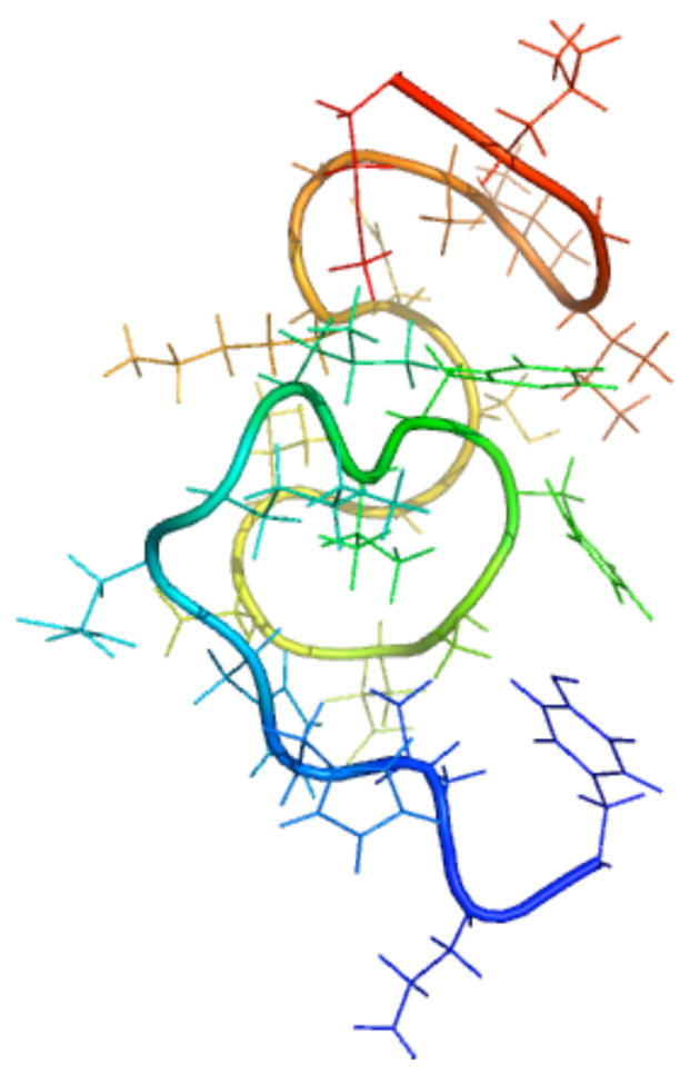
The amyloid beta peptide in the NMR derived conformation. The backbone is represented in tube format while the sidechain is shown in stick. (blue)-Tyr10-Glu11- Val12-His13-His14-Gln15-Lys16-Leu17-Val18-Phe19-Phe20-Ala21-Glu22-Asp23- Val24-Gly25-Ser26-Asn27-Lys28-Gly29-Ala30Ile31-Ile32-Gly33-Leu34-Met35-(red)

Self-Diffusion Constant

The self-diffusion constant is determined from the slope of the mean-square displacement of the center of mass of the peptide as a function time. To minimize averaging errors, the self-diffusion constant is determined from the most linear portion of the curve, i.e., from the 5–20 ns region of the 50 ns implicit trajectories and from the 2–8 ns region of the 10 ns MD trajectory.

End-to-End distance

The end-to-end distance of the peptide is taken as the distance between the nitrogen atom of the N terminal amino acid Tyr10 and the nitrogen atom between the two final residues. The end-to-end distance fluctuates in time mainly due to wagging of the ends.

Solvent Accessible Surface Area

The solvent accessible surface area is defined by the surface area of the atoms in the peptide that is accessible by a water probe with a radius of 1.4 Å following the method proposed by Lee and coworkers.^56,57

Radius of Gyration and RMSD

The radius of gyration is evaluated using the standard formula,

$$R_{G^2}\equiv \frac{\langle \sum _{i=1}^n{m}_i{(r_i-R)}^2\rangle }{\sum _{i=1}^n{m}_i},$$

with the sum ranging over every atom in the peptide. Here, R is the vector locating the center of mass of the molecule, r_i is the vector specifying the position of atom i with mass m_i. The root mean square deviations (RMSD) are determined with respect to the NMR derived structure.

NMR Order Parameter S²

The S² order parameter describes the range of internal motions of the NH amide bond vectors, being unity when this motion is completely restricted and vanishing when the amide bond vector experiences no restriction or undergoes isotropic movement. Because the protein is highly flexible, this parameter has been calculated following the strategy of Zhang and Brüschweiler that uses heavy atoms in neighboring residues to define a local environment for the N-H bond vector⁵⁸ rather than the standard Lipari-Szabo model free approach^59,60 in which the contribution from overall rigid-body molecular tumbling is removed by re-rotating and translating the peptide to the principal axes coordinate system. The Lipari-Szabo method generates order parameters that differ markedly between trajectories, in agreement with previous findings by Straub and coworkers,¹⁰ and from the new explicit solvent simulations. These strong fluctuations appear during an individual trajectory because the Lipari-Szabo method is designed only for much more rigid systems in which the internal motion can be separated from the overall rotation. More flexible peptides, such as Aβ(10–35), experience changes in the conformation of the backbone that are much more difficult to separate from strictly internal motions, and therefore the standard Lipari-Szabo equilibrium average formula generates order parameters that are artificially low for Aβ(10–35). By calculating the order parameter with respect to the residue’s immediate conformation and local environment, the overall motions have no effect. The two methods of calculating order parameters are compared (data not shown), and the Lipari-Szabo approach clearly provides a poorer representation of experiment. To benchmark the Zhang-Brüschweiler method, order parameters have been calculated from a ubiquitin LD trajectory of duration 5 ns and compared to available experimental data, yielding S² order parameters within 0.042 on average of experiments where typical values are S² ~ 0.6.⁶¹

Contacts

A “contact” between two residues is defined to occur when the O-H distance of the hydrogen bond is less than 5.4Å, as implemented by Han.⁷ The number of contacts between pairs of residues in each trajectory frame is accumulated to provide the average numbers of contacts during the trajectory. The contacts occurring within the ensemble of 15 “experimental” NMR conformations that are consistent with the measured constraints are represented in the lower half of the matrix below the diagonal to provide a comparison of computed and experimental values.

RESULTS

In this section, we compare several structural and dynamic properties obtained by averaging along the trajectories. These distributions are found to depend greatly on the choice of force field.⁴⁶ In addition, the implicit solvent models are applied using different initial structures to test the length required for equilibration. A comparison of properties between the all-atom implicit solvent LD and the explicit solvent simulations provides a rigorous validation for our implicit solvent model which can then be used for further studies of Aβ aggregation.

Self-Diffusion Constant

Table 1 and Fig. 2 summarize the computations for the translational diffusion constant from the four trajectories that begin from the NMR structure presented in Fig. 1. The diffusion constant obtained from the first ns of the explicit solvent trajectory is 3.82×10⁻⁶ cm² s⁻¹ and is 1.87×10⁻⁶ cm² s⁻¹ from the 2–8 ns region. The latter result agrees well with the measured 1.4×10⁻⁶ cm² s⁻¹ and with earlier simulations (1.6×10⁻⁶ cm² s^{− 1}).^25,26 Because the calculated diffusion constant varies with the portion of the trajectory used (see Table 1), it is essential that the trajectories are long enough to be equilibrated. The greater computational speed of the implicit solvent simulations enables a test of the equilibration times.

Table 1.

Diffusion Constants for trajectories with different force fields using NMR model as the initial structure.

Time Segment (ns)	CHARMM (×10−6)	CHARMM2 (×10−6)	OPLSaal (×10−6)	GARCIA (×10−6)	Explicit (×10−6)		Experiment (×10−6)
5–10	2.03	2.4	1.04	0.97	0–1 ns	3.82	1.4
10–15	2.7	2.95	1.11	1.1
15–20	3.32	3.18	1.51	0.79	2–8 ns	1.87
5–20	2.67	2.88	1.21	0.99
30–50	2.11	3.06	2.09	0.93

Figure 2.

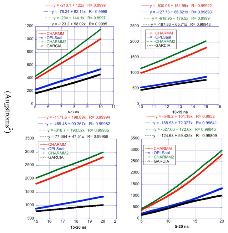
Plots of root-mean square displacement over time. Each panel corresponds to a different time segment of the trajectory which is the same as the label of the panel. The curves on each panel correspond to different force fields and are color coded as described in the legends of each panel. The equations of the fit are listed at the top of all the four panels for each force field. The slopes of the lines are 6D, where D is the diffusion constant in angstroms² ns⁻¹. These calculations were done only for trajectories starting with a model determined by NMR experiments.

The diffusion constant from implicit solvent simulations is calculated only for the trajectories that begin from the NMR initial structure to avoid possibly including contributions from large, stretched peptide conformations. The implicit solvent trajectory designated by CHARMM2 yields a diffusion coefficient closest to the explicit water simulations (Fig 2). However, the diffusion constants computed from the implicit solvent CHARMM trajectory is higher than experiment or those obtained from the explicit solvent simulation. One source of discrepancy could be the choice of the viscosity used in the LD simulations. Ideally, the viscosity should have been obtained form MD simulations for a box of TIP3P water molecules with the identical protocol (e.g. cutoff for non-bonded interactions) used for simulating amyloid-β(10–35). The other implicit solvent simulation using the CHARMM force field also yields a high diffusion constant (D= 2.03×10⁻⁶ for the 5–10 ns time segment); D from the GARCIA force field (D = 1.1×10⁻⁶ for the 10–15 ns time segment) is in modest agreement with experiment; while the OPLS-aal force field gives the best value (D = 1.51×10⁻⁶ for the 15–20 ns time segment) for the diffusion constant. Nevertheless, the LD and MD trajectories all produce similar diffusion constants to the experimental value. This good agreement with experiment provides support for the validity of the LD approach.

End-to-end Distance

Figure 3 presents the time variation of the end-to-end distances for all trajectories. The end-to-end distance from the 10 ns MD trajectory oscillates between a minimum of 10 Å and a maximum of over 40 Å, reflecting the flexibility of the molecule and the potential inaccuracy of using short simulations. Even at 10 ns the MD trajectory shows no evidence of having attained an equilibrated structure. In the first nanosecond alone, the end-to-end distance of the MD trajectory fluctuates over a range of 11.4 Å, which exceeds the width of distribution found through the Stokes-Einstein analysis method cited below. In comparison, Fig. 3 indicates that all LD trajectories attain a relatively equilibrated end-to-end distance (with minor fluctuations) after 30 ns.

Figure 3.

Time evolution of the end-to-end distance for the simulated trajectories. Each panel corresponds to a force field used and is the same as the labels of the panel. over time for all trajectories grouped by force field. The curves in each panel correspond to different starting structures for each simulation and are described in the legends.

Straub’s predicted end-to-end distance of 19.2 Ų⁵ from four 1 ns explicit solvent simulations is very close to our LD simulations: the highest for a well equilibrated structure is from the OPLS-aal trajectory with the initial NMR conformation and is centered around 20 Å, while the lowest (from the GARCIA and CHARMM simulations) dip to a lower limit of around 8 Å. The Stokes-Einstein analysis of quasielastic light scattering data method for calculating end-to-end distance used by Teplow and coworkers^20,21 yields even better agreement with our LD data, showing a distribution of radii between 10 and 20 Å. The probability distributions for the end-to-end distance from the equilibrated last 20 ns of the trajectories beginning from the NMR structure each exhibit a definite maximum peak but also a considerable width, suggesting a large range of motion of the peptide even after equilibration. The OPLS-aal trajectory with NMR initial structure has the narrowest distribution centered about 21 Å which is closest to Straub’s 19.2 Å prediction.²⁵

Radius of Gyration

The time dependence of the radius of gyration for all the LD trajectories beginning from the NMR structure is presented in Fig. 4. All trajectories agree very well with experimental. The 30 – 50 ns time slide of the trajectories beginning from the NMR structure all yield a somewhat lower average radius of gyration peaking at around 8.7 Å. Individually, they yield averages of 9.09 Å (GARCIA), 8.62 Å (CHARMM), 8.71 Å (OPLS-aal), and 8.53 Å (CHARMM2) and agree well with the hydrodynamic radius which is deduced from the diffusion constant as 10 Å using the Stokes-Einstein relation.²⁵

Figure 4.

Radii of gyration for the duration of each trajectory. Time evolution of the radius of gyration for the simulated trajectories. Each panel corresponds to a force field used and is the same as the labels of the panel. over time for all trajectories grouped by force field. The curves in each panel correspond to different starting structures for each simulation and are described in the legends.

The same behavior is found for the radius of gyration from the MD simulation. The radius of gyration grows by 30% over the NMR starting conformation within 4 ns and then returns towards the initial NMR value throughout the remainder of the trajectory, never again quite attaining the starting value by the end of 10 ns. The time variation of radius of gyration from the MD simulation indicates the peptide first expands and then slowly contracts again but does not equilibrate within 10 ns. The LD trajectories all equilibrate, the fastest (from the NMR initial condition) attains a stable radius of gyration by 10 ns, while the slowest (OPLS-aal stretched and GARCIA unfolded) require 30 ns for equilibration. The probability distributions for the radius of gyration from the last (equilibrated) 20 ns of the trajectories for the NMR initial structure display little difference between force fields except for the GARCIA force field, which yields a broader distribution centered ~ 0.2–0.3 Å above the others.

RMSD

The RMSD for each trajectory is presented as a function of time in Fig. 5 according to force field. Three terminal residues on either end of the peptide are ignored in this calculation due to the considerable wagging of the ends. All equilibrated trajectories remain within 8 Å RMSD of the NMR structure. Those beginning from the NMR structure all deviate by at least 3 Å, but stay within 6 Å RMSD of the initial structure. The CHARMM and CHARMM2 trajectories have the tightest distribution between 4.5 Å and 5.8 Å after equilibration, while the GARCIA and OPLS-aal trajectories produce a broader range of equilibrated RMSDs ranging from 4.5 Å to 6.7 Å. The trajectories run from random or stretched initial structures consistently have the worst agreement with NMR results. Some trajectories, especially the GARCIA trajectory from the unfolded initial structure, still undergo major fluctuations after 30 ns of simulation, suggesting some equilibration is still necessary. The large magnitude of the equilibrated RMSDs provides evidence that the peptide populates a large array of conformations even after equilibration.

Figure 5.

RMSD vs. time. The terminal residues (3 on either end of the peptide) were ignored during calculation of RMSD. Each panel corresponds to a force field used and is the same as the labels of the panel. over time for all trajectories grouped by force field. The curves in each panel correspond to different starting structures for each simulation and are described in the legends.

Solvent Accessible Surface Area

Several structural and computational studies of the amyloid-β peptide display the presence of a hydrophobic exposed patch and discuss the role of this patch in the mechanism of aggregation of the peptides to form plaque.^6,7,9,24 Thus, we now investigate the solvent accessible surface area (SASA) for the hydrophobic LVFFA core region as well as the for the whole peptide (Fig. 6). The MD trajectory produces a wide range of surface areas in just 10 ns, first rising steeply to twice the starting value and then dropping back down after 4 ns for both the LVFFA region and the whole peptide, indicating a relatively fast unfolding process followed by a slower re-folding. The slope of the latter part of this trajectory indicates that the peptide may return to a SASA something close to the NMR value at longer times.

Figure 6.

Solvent accessible surface area for the LVFFA region vs. time. Each panel corresponds to a force field used and is the same as the labels of the panel. over time for all trajectories grouped by force field. The curves in each panel correspond to different starting structures for each simulation and are described in the legends.

The LVFFA regions of the OPLS-aal and GARCIA LD trajectories equilibrate to a variety of structures with SASAs ranging from between 300 and 650 Ų, while the CHARMM LD trajectories produce a narrower distribution of SASAs between 350 and 550 Ų. The SASAs for the whole protein remain between 2300 and 3000 Ų for all LD trajectories, exhibiting good agreement with NMR data (SASA = 2315 Ų, averaged from NMR ensemble). For the LVFFA region, the CHARMM force field trajectories equilibrate to more constant SASAs than the trajectories run with OPLSaal or GARCIA, and there are only minor differences between the SASAs from the different force fields. Again, the SASAs for most trajectories fluctuate even after 30 ns, indicating significant structural changes within the equilibrated state.

When the trajectories starting from a stretched initial position, over half of the SASA in the initial configuration for the LVFFA region remains exposed to the solvent. As reported by Zhang et al., the exposure of the hydrophobic region of the peptide is essential for the aggregation and fibril formation mechanism.²⁴ All of our LD implicit solvent trajectories, regardless of initial structure, display the LVFFA region as to a large degree remaining exposed to the solvent, thus agreeing with the ensemble of structures derived from NMR experiments. Figure 7 depicts the percent of the total exposed surface area comprised by the LVFFA region for all trajectories that begin from a stretched initial structure. The hydrophobic patch may be expected to become buried as the peptide folds in upon itself. However, the relative exposed surface area of this region remains constant or even, for the OPLS-aal trajectory, increases to around 25% of the total. Including all exposed hydrophobic residues, the total contribution to the SASA from the last equilibrated 20 ns of trajectories (with NMR initial condition) ranges between 43 % (CHARMM) and 50 % (OPLS-aal) of the total, so the 1/3 total described by Zhang et al. is consistent with our range of hydrophobic contributions to the SASA.

Figure 7.

Same as 6 but for the entire peptide.

S² Order Parameter

The order parameter is presented for all trajectories in Fig. 8 as well as in table 2. The S² order parameter varies from 0 to 1 and describes the range of internal motions of the NH amide bond vectors, where S²=1 corresponds to the case of an immobile NH bond vector while S²=0 suggests that the amide bond vector experiences no restriction or undergoes isotropic movement. Use of the standard Lipari-Szabo model free approach yields very poor agreement with experiments, and the calculated order parameters differ widely among different trajectories in general accord with the calculations of Straub. Since the protein is highly flexible, it is not possible to eliminate contributions from overall rigid-body molecular tumbling by re-rotating and translating the peptide to its principal axes coordinate system. Consequently, the Lipari-Szabo model free approach fails to provide consistent order parameters for the residues in amyloid-β(10–35).

Figure 8.

Averaged S² order parameters for the last 20 ns of each trajectory. The strategy of Zhang and Brüschweiler that uses heavy atoms in neighboring residues to define a local environment for the N-H bond vector⁵⁸ was used to estimate the order parameter from simulated trajectories. The residues for which experimental data is available is also shown on the plot.

Table 2.

Order Parameter predictions for all force fields and the explicit trajectory compared to experiment.

Residue	CHARMM	CHARMM2	GARCIA	OPLSaal	Explicit	Experiment
2	0.40	0.47	0.33	0.49	0.18
3	0.76	0.78	0.78	0.75	0.60
4	0.80	0.72	0.80	0.87	0.81
5	0.80	0.66	0.80	0.89	0.67
6	0.52	0.82	0.87	0.85	0.69
7	0.71	0.67	0.88	0.76	0.70
8	0.63	0.79	0.84	0.80	0.78
9	0.64	0.84	0.81	0.79	0.76	0.68±0.05
10	0.78	0.85	0.87	0.88	0.79	0.75±0.05
11	0.77	0.85	0.87	0.88	0.64	0.79±0.05
12	0.76	0.87	0.84	0.83	0.55
13	0.78	0.83	0.80	0.82	0.56
14	0.58	0.75	0.59	0.74	0.57
15	0.70	0.63	0.74	0.79	0.71	0.75±0.05
16	0.81	0.68	0.77	0.88	0.72	0.76±0.05
17	0.74	0.84	0.85	0.90	0.77
18	0.72	0.82	0.85	0.83	0.71
19	0.82	0.78	0.78	0.86	0.74
20	0.73	0.80	0.85	0.86	0.78	0.64±0.06
21	0.62	0.78	0.88	0.87	0.60
22	0.66	0.84	0.89	0.68	0.63
23	0.84	0.85	0.83	0.82	0.52
24	0.86	0.86	0.85	0.83	0.61	0.54±0.06
25	0.82	0.77	0.81	0.76	0.67
26	0.62	0.54	0.59	0.68	0.49

We therefore adopt the strategy of Zhang and Brüschweiler that uses heavy atoms in neighboring residues to define a local environment for the N-H bond vector⁵⁸ in order to estimate the order parameter from simulated trajectories. To benchmark the Zhang- Brüschweiler method, order parameters have been calculated from a ubiquitin LD trajectory of duration 5 ns and have been compared to available experimental data,⁶¹ (data not shown) yielding excellent agreement. While the Lipari-Szabo model for the flexible peptide Aβ(10–35) generates order parameters that are artificially low, the order parameters determined from the Zhang and Brüschweiler approach for most of the trajectories agree well with each other and with experiment. The MD trajectory calculations (only in table 2) perform on par with the other LD trajectories for the residues for which experimental data are available. All the trajectories exhibit the presence of a structured region (see contact maps below) from residues 17–23 relative to the carboxy and amino terminus of the protein. However, the amino terminus of amyloidβ(10–35) seems to be more unstructured than the carboxy terminus. The structural interpretation of these trends of S² as a function of sequence suggests that there is a structured hydrophobic core and some residues from the carboxy end form what can be called the extended core (residues 16–30) of the peptide. The amino end of the peptide, however, has highly mobile amide bond vectors because the ends are freer to move or adopt different conformations that would affect the end residues’ order parameters. The agreement between different force fields is good except CHARMM consistently predicts smaller values of S² for most of the residues. However, the CHARMM trajectory yields excellent agreement with five of the seven residues for which experimental values are available. The worst fit of the trajectories to experiment occurs in the last two residues, Gly29 and Gly33, for which experimental data are available. The agreement with experiment for S² must be interpreted cautiously because the experimental S² have been measured at a pH of 5.7 and because of evidence displaying a pH dependence of these measurements.⁶² Our simulations probably correspond best to neutral pH. Moreover, the experimental order parameters have been obtained using Lipari-Szabo model free approach.

Contacts

Contacts between residues are represented in the contact matrices of Fig. 9. The axes indicate the residues sequentially, beginning with Tyr10. The intensity is a qualitative measure of the contact between two residues, averaged over last 20 ns of the trajectory. The range of white to red indicates the percentage of frames with contacts at that location, from 0 to 100% respectively. The bottom right halves of each graph are the contact maps for the ensemble of NMR structures, which serve as a reference for comparison with simulations. Figure 9 indicates that the most obvious consistency between the force fields is their prediction of contacts between residues that are not immediate neighbors in the peptide sequence, shown as a diagonal line from (10,10) to (35,35) with positive slope on the contact matrix. A turn of varying degrees is apparent in each matrix, as evidenced by a diagonal with negative slope and midpoint near the 15^th residue in the sequence and most prominent in the GARCIA trajectory. The longer this diagonal, the more contacts between opposite sides of the peptide equidistant from the center of the loop, suggesting a collapsed-coil or strand-loop-strand structure, a conformation also found in experiment as well as other recent simulations.^6,7,9

Figure 9.

Contact matrices for the last 20 ns of trajectories starting from NMR. The bottom half below the diagonal serves as a reference and shows the contact matrix obtained from the NMR ensemble. Each panel corresponds to the force field that was used to generate the given trajectory.

The CHARMM and CHARMM2 LD trajectories show a large number of contacts near the C-terminus, indicating that this end is bent back towards the center of the molecule. The horizontal line on the upper region of the contact matrix for the CHARMM trajectory indicates that the C terminus end of the peptide turns back very near the center of the molecule, enabling the 24^th and 25^th residues to contact nearly all other residues in the molecule. However, these contacts are not present in the other trajectories, indicating that the other force fields allow this end to move more freely and away from the rest of the molecule.

Clearly, the protein displays a large degree of conformational fluctuations, supporting its propensity to aggregate. The large discrepancies between each matrix suggest an array of structures for the β-amyloid(10–35) monomer. The change in dielectric constant alone between the CHARMM and CHARMM2 LD simulations drastically alters the contacts formed and mirrors the discrepancies in other measures because this variability arises due to the flexibility of the peptide.

SUMMARY and CONCLUSIONS

A number of LD simulations have been performed using three different force fields, GARCIA, OPLS-aal, and CHARMM. The simulations have been used to calculate various properties of the peptide that describe its structure, dynamics, and conformational restraints. Comparisons with experiment help assess the accuracy and strengths of the different force fields.

The simulations quite accurately represent experimental data for all properties calculated. The diffusion constant varies somewhat between force fields, but never strays enough to be indicative of improper protein conformations or errors in the LD technique. The fact that any initial conformation, even the incredibly energetically unfavorable stretched conformation, eventually folds to something close to the naturally occurring peptide structure, provides good support for our LD method. The different force fields only yield subtle differences in the computed RMSD, radius of gyration, end-to-end distance, and solvent accessible surface area.

Other than the NMR order parameter, the properties determined here all reflect large scale, overall motion and structure. The NMR order parameter, on the other hand, is sensitive to the much more local motions of the backbone NH bond vectors individually. The Zhang-Brüschweiler method for calculating the NMR order parameter is much more successful in reproducing experiment than the correlation function approach because the latter is much more suited to determining order parameters for flexible molecules whose inertial frames change too much for the separation of internal motion from overall rotation. The excellent agreement of our LD trajectories with experiment for the NMR order parameters provides additional support for the success of our LD method. Furthermore, the variation in the computed NMR order parameters with force fields again stress the need for refinement of force fields for treating flexible portions of proteins.

The predictions from the MD trajectory are no better than those from the 170 times faster LD trajectories. In fact, the LD simulations yield better diffusion constant and NMR order parameters than the not fully equilibrated MD trajectory. This decrease in computational cost will be more significant for future simulations of the aggregation mechanism and dynamics.

Our simulations display the peptide as attaining a loosely defined strand-loop-strand structure suggested in recent work, while retaining a large amount of flexibility. The large NMR order parameters for the central LVFFA region indicate a relatively stable internal structure, a conclusion further supported by the large number of contacts in the same region. Contacts of the C-terminus with the rest of the molecule also reflect the bend of this end towards the central hydrophobic core. Furthermore, the hydrophobic LVFFA region is always largely exposed to the solvent, a very important characteristic for the aggregation of the molecule. Future simulations of multiple peptides will be useful to reveal the details of the aggregation process and the key role of the central hydrophobic region.

Equilibration ensues only after as much as 30 ns of simulation. The fastest equilibrating simulations are those starting from NMR, a structure that should already be very close to equilibrium. However, even these simulations, for both implicit and explicit solvents, display significant fluctuations for up to 10 ns. Thus any trajectory shorter than 10 ns, and perhaps even 30 ns, is of questionable value for describing equilibrium properties of Aβ(10–35) despite any apparent similarities between the simulation and experiment.

The differences in computed properties, especially the diffusion constant and NMR order parameter, from the three force fields stress the need for care in the choice of force field and for their further improvement. The implicit solvent model is particularly useful for screening force fields due to its far greater computational speed than explicit solvent MD simulations. Because our LD simulations agree both with experiment and MD simulations, we are extremely well positioned to study the aggregation dynamics.

References

- 1.Pillot T, Drouet B, Queille S, Labeur C, Vandekerckhove J, Rosseneu M, Pincon-Raymond M, Chambaz J. Journal of Neurochemistry. 1999;73:1626. doi: 10.1046/j.1471-4159.1999.0731626.x. [DOI] [PubMed] [Google Scholar]
- 2.Lambert MP, Barlow AK, Chromy BA, Edwards C, Freed R, Liosatos M, Morgan TE, Rozovsky I, Trommer B, Viola KL, Wals P, Zhang C, Finch CE, Krafft GA, Klein WL. Proceedings of the National Academy of Sciences of the United States of America. 1998;95:6448. doi: 10.1073/pnas.95.11.6448. [DOI] [PMC free article] [PubMed] [Google Scholar]
- 3.Selkoe DJ. Journal of Neuropathology and Experimental Neurology. 1994;53:438. doi: 10.1097/00005072-199409000-00003. [DOI] [PubMed] [Google Scholar]
- 4.Kelly JW. Current Opinion in Structural Biology. 1998;8:101. doi: 10.1016/s0959-440x(98)80016-x. [DOI] [PubMed] [Google Scholar]
- 5.Borreguero JM, Urbanc B, Lazo ND, Buldyrev SV, Teplow DB, Stanley HE. Proceedings of the National Academy of Sciences of the United States of America. 2005;102:6015. doi: 10.1073/pnas.0502006102. [DOI] [PMC free article] [PubMed] [Google Scholar]
- 6.Luttmann E, Fels G. Chemical Physics. 2006;323:138. [Google Scholar]
- 7.Han W, Wu YD. Journal of the American Chemical Society. 2005;127:15408. doi: 10.1021/ja051699h. [DOI] [PubMed] [Google Scholar]
- 8.Cecchini M, Rao F, Seeber M, Caflisch A. Journal of Chemical Physics. 2004;121:10748. doi: 10.1063/1.1809588. [DOI] [PubMed] [Google Scholar]
- 9.Klimov DK, Thirumalai D. Structure. 2003;11:295. doi: 10.1016/s0969-2126(03)00031-5. [DOI] [PubMed] [Google Scholar]
- 10.Massi F, Straub JE. Journal of Computational Chemistry. 2003;24:143. doi: 10.1002/jcc.10101. [DOI] [PubMed] [Google Scholar]
- 11.Melquiond A, Gelly JC, Mousseau N, Derreumaux P. Journal of Chemical Physics. 2007:126. doi: 10.1063/1.2435358. [DOI] [PubMed] [Google Scholar]
- 12.Straub JE, Guevara J, Huo SH, Lee JP. Accounts of Chemical Research. 2002;35:473. doi: 10.1021/ar010031e. [DOI] [PubMed] [Google Scholar]
- 13.Baumketner A, Bernstein SL, Wyttenbach T, Bitan G, Teplow DB, Bowers MT, Shea JE. Protein Science. 2006;15:420. doi: 10.1110/ps.051762406. [DOI] [PMC free article] [PubMed] [Google Scholar]
- 14.Jang S, Shin S. Journal of Physical Chemistry B. 2006;110:1955. doi: 10.1021/jp055568e. [DOI] [PubMed] [Google Scholar]
- 15.Walsh DM, Hartley DM, Kusumoto Y, Fezoui Y, Condron MM, Lomakin A, Benedek GB, Selkoe DJ, Teplow DB. Journal of Biological Chemistry. 1999;274:25945. doi: 10.1074/jbc.274.36.25945. [DOI] [PubMed] [Google Scholar]
- 16.Zhu YJ, Lin H, Lal R. Faseb Journal. 2000;14:1244. doi: 10.1096/fasebj.14.9.1244. [DOI] [PubMed] [Google Scholar]
- 17.Kayed R, Head E, Thompson JL, McIntire TM, Milton SC, Cotman CW, Glabe CG. Science. 2003;300:486. doi: 10.1126/science.1079469. [DOI] [PubMed] [Google Scholar]
- 18.Bitan G, Vollers SS, Teplow DB. Journal of Biological Chemistry. 2003;278:34882. doi: 10.1074/jbc.M300825200. [DOI] [PubMed] [Google Scholar]
- 19.Hartley DM, Walsh DM, Ye CPP, Diehl T, Vasquez S, Vassilev PM, Teplow DB, Selkoe DJ. Journal of Neuroscience. 1999;19:8876. doi: 10.1523/JNEUROSCI.19-20-08876.1999. [DOI] [PMC free article] [PubMed] [Google Scholar]
- 20.Lomakin A, Chung DS, Benedek GB, Kirschner DA, Teplow DB. Proceedings of the National Academy of Sciences of the United States of America. 1996;93:1125. doi: 10.1073/pnas.93.3.1125. [DOI] [PMC free article] [PubMed] [Google Scholar]
- 21.Lomakin A, Teplow DB, Kirschner DA, Benedek GB. Proceedings of the National Academy of Sciences of the United States of America. 1997;94:7942. doi: 10.1073/pnas.94.15.7942. [DOI] [PMC free article] [PubMed] [Google Scholar]
- 22.Gordon DJ, Sciarretta KL, Meredith SC. Biochemistry. 2001;40:8237. doi: 10.1021/bi002416v. [DOI] [PubMed] [Google Scholar]
- 23.Gordon DJ, Tappe R, Meredith SC. Journal of Peptide Research. 2002;60:37. doi: 10.1034/j.1399-3011.2002.11002.x. [DOI] [PubMed] [Google Scholar]
- 24.Zhang S, Iwata K, Lachenmann MJ, Peng JW, Li S, Stimson ER, Lu Y, Felix AM, Maggio JE, Lee JP. Journal of Structural Biology. 2000;130:130. doi: 10.1006/jsbi.2000.4288. [DOI] [PubMed] [Google Scholar]
- 25.Massi F, Peng JW, Lee JP, Straub JE. Biophysical Journal. 2001;80:31. doi: 10.1016/S0006-3495(01)75993-0. [DOI] [PMC free article] [PubMed] [Google Scholar]
- 26.Tseng BP, Esler WP, Clish CB, Stimson ER, Ghilardi JR, Vinters HV, Mantyh PW, Lee JP, Maggio JE. Biochemistry. 1999;38:10424. doi: 10.1021/bi990718v. [DOI] [PubMed] [Google Scholar]
- 27.Zanuy D, Gunasekaran K, Ma BY, Tsai HH, Tsai CJ, Nussinov R. Amyloid-Journal of Protein Folding Disorders. 2004;11:143. doi: 10.1080/13506120400000798. [DOI] [PubMed] [Google Scholar]
- 28.Massi F, Straub JE. Biophysical Journal. 2001;81:697. doi: 10.1016/S0006-3495(01)75734-7. [DOI] [PMC free article] [PubMed] [Google Scholar]
- 29.Buchete NV, Tycko R, Hummer G. Journal of Molecular Biology. 2005;353:804. doi: 10.1016/j.jmb.2005.08.066. [DOI] [PubMed] [Google Scholar]
- 30.Derreumaux P, Mousseau N. Journal of Chemical Physics. 2007:126. doi: 10.1063/1.2408414. [DOI] [PubMed] [Google Scholar]
- 31.Shen MY, Freed KF. Biophysical Journal. 2002;82:1791. doi: 10.1016/s0006-3495(02)75530-6. [DOI] [PMC free article] [PubMed] [Google Scholar]
- 32.Shen MY, Freed KF. Proteins-Structure Function and Genetics. 2002;49:439. doi: 10.1002/prot.10230. [DOI] [PubMed] [Google Scholar]
- 33.Brooks BR, Bruccoleri RE, Olafson BD, States DJ, Swaminathan S, Karplus M. Journal of Computational Chemistry. 1983;4:187. [Google Scholar]
- 34.Shen MY, Freed KF. Journal of Computational Chemistry. 2005;26:691. doi: 10.1002/jcc.20211. [DOI] [PubMed] [Google Scholar]
- 35.Still WC, Tempczyk A, Hawley RC, Hendrickson T. Journal of the American Chemical Society. 1990;112:6127. [Google Scholar]
- 36.Pastor RW, Karplus M. Journal of Physical Chemistry. 1988;92:2636. [Google Scholar]
- 37.Shen MY. Computer Simulations of Protein Dynamics. University of Chicago; 2002. [Google Scholar]
- 38.Bursulaya BD, Brooks CL. Journal of Physical Chemistry B. 2000;104:12378. [Google Scholar]
- 39.Pak Y, Kim E, Jang S. Journal of Chemical Physics. 2004;121:9184. doi: 10.1063/1.1804159. [DOI] [PubMed] [Google Scholar]
- 40.Zhou RH. Proteins-Structure Function and Genetics. 2003;53:148. [Google Scholar]
- 41.Zhou RH, Berne BJ. Proceedings of the National Academy of Sciences of the United States of America. 2002;99:12777. doi: 10.1073/pnas.142430099. [DOI] [PMC free article] [PubMed] [Google Scholar]
- 42.Baumketner A, Shea JE. Physical Review E. 2003:68. doi: 10.1103/PhysRevE.68.051901. [DOI] [PubMed] [Google Scholar]
- 43.Mallik B, Masunov A, Lazaridis T. Journal of Computational Chemistry. 2002;23:1090. doi: 10.1002/jcc.10104. [DOI] [PubMed] [Google Scholar]
- 44.Guo W, Shea JE, Berry RS. Submitted. [Google Scholar]
- 45.Bucciantini M, Giannoni E, Chiti F, Baroni F, Formigli L, Zurdo JS, Taddei N, Ramponi G, Dobson CM, Stefani M. Nature. 2002;416:507. doi: 10.1038/416507a. [DOI] [PubMed] [Google Scholar]
- 46.Zaman MH, Shen MY, Berry RS, Freed KF, Sosnick TR. J Mol Biol. 2003;331:693. doi: 10.1016/s0022-2836(03)00765-4. [DOI] [PubMed] [Google Scholar]
- 47.Foloppe N, MacKerell AD. Journal of Computational Chemistry. 2000;21:86. [Google Scholar]
- 48.MacKerell AD, Bashford D, Bellott M, Dunbrack RL, Evanseck JD, Field MJ, Fischer S, Gao J, Guo H, Ha S, Joseph-McCarthy D, Kuchnir L, Kuczera K, Lau FTK, Mattos C, Michnick S, Ngo T, Nguyen DT, Prodhom B, Reiher WE, Roux B, Schlenkrich M, Smith JC, Stote R, Straub J, Watanabe M, Wiorkiewicz-Kuczera J, Yin D, Karplus M. Journal of Physical Chemistry B. 1998;102:3586. doi: 10.1021/jp973084f. [DOI] [PubMed] [Google Scholar]
- 49.Andersen HC. Journal of Computational Physics. 1983;52:24. [Google Scholar]
- 50.Vorobjev YN, Hermans J. Biophysical Chemistry. 1999;78:195. doi: 10.1016/s0301-4622(98)00230-0. [DOI] [PubMed] [Google Scholar]
- 51.Ramstein J, Lavery R. Proceedings of the National Academy of Sciences of the United States of America. 1988;85:7231. doi: 10.1073/pnas.85.19.7231. [DOI] [PMC free article] [PubMed] [Google Scholar]
- 52.Jha A, Freed KF. Solvation effect on conformations of 1,2:Dimethoxyethane: Charge dependent nonlinear response in implicit solvent models. doi: 10.1063/1.2815764. Submitted. [DOI] [PMC free article] [PubMed] [Google Scholar]
- 53.Ooi T, Oobatake M, Nemethy G, Scheraga HA. Proceedings of the National Academy of Sciences of the United States of America. 1987;84:3086. doi: 10.1073/pnas.84.10.3086. [DOI] [PMC free article] [PubMed] [Google Scholar]
- 54.Allen MP, Tildesley DJ. Computer simulation of liquids. Clarendon Press; Oxford University Press; Oxford England New York: 1989. [Google Scholar]
- 55.Jha AK, Colubri A, Freed KF, Sosnick TR. Proceedings of the National Academy of Sciences of the United States of America. 2005;102:13099. doi: 10.1073/pnas.0506078102. [DOI] [PMC free article] [PubMed] [Google Scholar]
- 56.Lee B, Richards FM. Journal of Molecular Biology. 1971;55:379. doi: 10.1016/0022-2836(71)90324-x. [DOI] [PubMed] [Google Scholar]
- 57.Wesson L, Eisenberg D. Protein Science. 1992;1:227. doi: 10.1002/pro.5560010204. [DOI] [PMC free article] [PubMed] [Google Scholar]
- 58.Zhang FL, Bruschweiler R. Journal of the American Chemical Society. 2002;124:12654. doi: 10.1021/ja027847a. [DOI] [PubMed] [Google Scholar]
- 59.Lipari G, Szabo A. Journal of the American Chemical Society. 1982;104:4546. [Google Scholar]
- 60.Lipari G, Szabo A. Journal of the American Chemical Society. 1982;104:4559. [Google Scholar]
- 61.Wand AJ, Urbauer JL, McEvoy RP, Bieber RJ. Biochemistry. 1996;35:6116. doi: 10.1021/bi9530144. [DOI] [PubMed] [Google Scholar]
- 62.Laus S, Sour A, Ruloff R, Toth E, Merbach AE. Chemistry-a European Journal. 2005;11:3064. doi: 10.1002/chem.200401326. [DOI] [PubMed] [Google Scholar]