

Abstract
A sharp interface immersed boundary method for simulating incompressible viscous flow past three-dimensional immersed bodies is described. The method employs a multi-dimensional ghost-cell methodology to satisfy the boundary conditions on the immersed boundary and the method is designed to handle highly complex three-dimensional, stationary, moving and/or deforming bodies. The complex immersed surfaces are represented by grids consisting of unstructured triangular elements; while the flow is computed on non-uniform Cartesian grids. The paper describes the salient features of the methodology with special emphasis on the immersed boundary treatment for stationary and moving boundaries. Simulations of a number of canonical two- and three-dimensional flows are used to verify the accuracy and fidelity of the solver over a range of Reynolds numbers. Flow past suddenly accelerated bodies are used to validate the solver for moving boundary problems. Finally two cases inspired from biology with highly complex three-dimensional bodies are simulated in order to demonstrate the versatility of the method.
Keywords: computational fluid dynamics, immersed boundary method, ghost cell, body non-conformal grid methods
1 Introduction
Immersed boundary methods have emerged in recent years as a viable alternative to conventional body-conformal grid methods especially in problems involving complex stationary and/or moving boundaries. For such flows, the elimination of the need to establish a new body-conformal grid at each time-step can significantly simplify and speedup the solution procedure and also eliminates issues associated with regridding such as grid-quality and grid-interpolation errors. Immersed boundary methods can broadly be characterized under two categories [29]; first is the category of methods that employ “continuous forcing” wherein a forcing term is added to the continuous Navier-Stokes equations before they are discretized. Methods such as those of Peskin[36], Goldstein et al.[13] and Saiki and Biringen[39] fall in this category.
The second category consists of methods that employ discrete forcing where the forcing is either explicitly or implicitly applied to the discretized Navier-Stokes equations. These include methods of Udaykumar et al.[44], Ye et al.[51], Fadlun et al. [9], Kim et al. [16], Gibou et al.[12], You et al.[52], Balaras [2], Marella et al.[22], Ghias et al.[11] and others. The key advantage of the first category of methods is that they are formulated relatively independent of the spatial discretization and therefore can be implemented into an existing Navier-Stokes solver with relative ease. However, one of their drawbacks is that they produce a “diffuse” boundary. This means that the boundary condition on the immersed surface is not precisely satisfied at its actual location but within a localized region around the boundary. For the methods in the second category, the forcing scheme is very much dependent on the spatial discretization. However, one key advantage of the second category of methods is that for certain formulations, they allow for a sharp representation of the immersed boundary.
In the current paper, we describe a finite-difference based immersed boundary method that allows us to simulate incompressible flows with complex three-dimensional stationary or moving immersed boundaries on Cartesian grids that do not conform to the immersed boundary. The current method is based on the calculation of the variables on “ghost-cells” inside the body such that the boundary conditions are satisfied precisely on the immersed boundary. There are no ad-hoc constants introduced in this procedure and neither is any momentum forcing term employed in any of the fluid cells. Consequently, the method results in a sharp representation of the immersed boundary. The method is designed from the ground up for simulations of flow with complex, moving, three-dimensional boundaries such as those encountered in bio-fluid mechanics and this paper describes the salient features of the methodology. The solver is validated by simulating a number of canonical two- (2D) and three-dimensional (3D) flows with stationary and moving boundaries, and comparing with established computed and/or experimental data. We also verify the spatial accuracy of the solver through a grid refinement study. Finally in order to showcase the capability of the method for handling general immersed boundaries, we present some computed results for flow with highly complex, non-canonical geometries.
The paper is organized as follows: Section 2 describes the numerical methodology including a detailed description of underlying flow solver and the overlaid immersed boundary methodology. In Section 3 we present computed results for a broad range of cases that are intended to validate the solver and to firmly establish its accuracy. In this section we also include qualitative results from two biologically inspired simulations that involve highly complex moving/deforming bodies and these are meant to demonstrate the ability of the solver to handle complex immersed bodies. Finally, conclusions are presented in Section 4.
2 Numerical Method
2.1 Governing Equations and Discretization Scheme
The governing equations considered are the 3-D unsteady Navier-Stokes equations for a viscous incompressible flow with constant properties given by
| (1) |
| (2) |
where i; j = 1, 2, 3, ui are the velocity components, p is the pressure, and where ρ and ν are the fluid density and kinematic viscosity.
The Navier-Stokes equations (2) are discretized using a cell-centered, collocated (non-staggered) arrangement of the primitive variables (ui, p). In addition to the cell-center velocities (ui), the face-center velocities, Ui, are computed. The equations are integrated in time using the fractional step method of Van-Kan [46] which consists of three sub-steps. In the first sub-step of this method, a modified momentum equation is solved and an intermediate velocity u* obtained. A second-order, Adams-Bashforth scheme is employed for the convective terms while the diffusion terms are discretized using an implicit Crank-Nicolson scheme which eliminates the viscous stability constraint. In this sub-step, the following modified momentum equation is solved at the cell-nodes
| (3) |
where and are the convective and diffusive terms respectively, and corresponds to a second-order central difference. This equation is solved using a line-SOR scheme. Subsequently, face-center velocities at this intermediate step U* are computed by averaging the corresponding values at the grid nodes. Similar to a fully staggered arrangement, only the face velocity component normal to the cell-face is calculated and used for computing the volume flux from each cell. The following averaging procedure is followed:
| (4) |
| (5) |
| (6) |
| (7) |
| (8) |
where γw, γs and γb are the weights corresponding to linear interpolation for the west, south and back face velocity components respectively. Furthermore, cc and fc denote gradients computed at cell-centers and face-centers respectively. The above procedure is necessary to eliminate odd-even decoupling that usually occurs with non-staggered methods and which leads to large pressure variations in space. The second sub-step requires the solution of the pressure correction equation
| (9) |
which is solved with the constraint that the final velocity be divergence-free. This gives the following Poisson equation for the pressure correction
| (10) |
and a Neumann boundary condition imposed on this pressure correction at all boundaries. This Poisson equation is solved with a highly efficient geometric multigrid method [3] which employs a Gauss-Siedel line-SOR smoother [38]. Once the pressure correction is obtained, the pressure and velocity are updated as
| (11) |
| (12) |
| (13) |
These separately updated face-velocities satisfy discrete mass-conservation to machine accuracy and use of these velocities in estimating the non-linear convective flux in equation (3) leads to a more accurate and robust solution procedure. The advantage of separately computing the face-center velocities was initially proposed by Zang et al. [53] and discussed in the context of the Cartesian grid methods in Ye et al. [51].
2.2 Immersed Boundary Treatment
The current immersed boundary method employs a multi-dimensional ghost-cell methodology to impose the boundary conditions on the immersed boundary and is similar in spirit to the methodology proposed by Majumdar et al.[21] and employed by Ghias et al. [10,11] among others. However, unlike these previous efforts, the current solver is designed from the start for fast, efficient and accurate solution of flows with complex three-dimensional, moving boundaries. In Ghias et al.[11] in particular, similar ideas have been used for simulating compressible flows with 2D stationary immersed boundaries. As discussed in detail in that paper, the methodology used here has a general similarity to the ghost-fluid method of Gibou et al. [12] which also employs ghost-cells for imposing the boundary conditions on the immersed boundary. However there are some key differences between the two methodologies and these will be discussed briefly later in the paper.
Within the context of the categorization put forth by Mittal & Iaccarino [29], this method employs a “discrete forcing” method wherein the effect of the immersed boundary is incorporated into the discretized governing equations. This is in contrast to methods such as that of Peskin[36] and others that incorporate the momentum forcing into the continuous equations and then discretize this modified equation. The current method is a “sharp” interface method in that the boundary conditions on the immersed boundary are imposed at the precise location of the immersed body and there is no spurious spreading of boundary forcing into the fluid as what usually occurs with diffuse interface methods [29]. In the rest of this section we provide an overview of the salient features of this method.
2.2.1 Geometric Representation of Immersed Boundary
The current method is designed to simulate flows over arbitrarily complex 2D and 3D immersed stationary and moving boundaries and the approach chosen to represent the boundary surface should be flexible enough so as not to limit the type of geometries that can be handled. In addition, the surface representation method should be such as not to lead to excessive computational overhead (in terms of both memory and CPU time) for geometric operations associated with the immersed boundary(IB) surface. Finally, another factor to be considered here is the compatibility between the current solver and CAD programs which oftentimes provide the geometry of the immersed boundary and other pre- and post-processing softwares such as Alias MAYA [8] (animation), Rhino [7] (surface modeling and modification) and Tecplot (visualization) which are useful in the modeling and articulation of the geometries and analysis of these complex flows.
A number of different approaches are available for representing the surface of the immersed boundary including level-sets [35], NURBS [37] and unstructured surface meshes [5]. In the current solver we choose to represent the surface of the IB by a unstructured mesh with triangular elements. This approach is very well suited for the wide variety of engineering and biological flow configurations that we are interested and as will become clear later in the paper, is very compatible with the immersed boundary methodology used in the current solver.
Many fast and efficient algorithms exist for generation of such meshes [4,23] and accurate and efficient representation of surfaces can be obtained through the use of non-uniform, non-isotropic meshes. Figure 2 shows the surface mesh over a porpoise which is being use to examine the fluid dynamics of drafting in cetaceans and the figure shows how the surface mesh non-uniformity allows us to provide enhanced resolution in regions such as the flippers that have finer geometric features. Because of these capabilities such meshes are ubiquitous in computational mechanics and virtually all commercial solid modeling, CAD, rapid prototyping, animation, graphics and visualization softwares are able to take input and/or provide output in this format. Such surface meshes are also easy to modify through operations such as smoothing, triangle subdivision/decimation and surface properties such as areas and normals are also available through simple operations. Finally, level-set representations can be obtained from the surface mesh quite easily if needed.
Fig. 2.

Example of the type of surface mesh with triangular elements used to represent all immersed bodies in the current solver. This particular body is based on a CT scan of a harbor porpoise (Phocoena phocoena).
2.2.2 Ghost-Cell Formulation
The unstructured surface mesh is “immersed” into the Cartesian volume grid and Fig. 3 shows this for the particular case of the body in Fig. 2. The next step is to develop all the computational machinery that is needed to implement the ghost-cell methodology for such an immersed boundary. The method proceeds by first identifying cells whose nodes are inside the solid boundary (termed “solid cells”) and cells that are outside the body (termed “fluid cells”). A straightforward method for this as depicted in Fig. 4 is to determine the surface element closest to a given node and taking a dot-product of the vector extending from this element to the node with the surface normal of this element . A positive(negative) value of the dot-product then indicates that the node is outside(inside) the body. For stationary boundaries, this determination needs to be done just once at the beginning of the simulation and therefore represents only a small fraction of the total turnaround time. For moving boundaries, this determination needs to be done at every time-step. However given that the immersed boundary can only travel a distance of the order of the nominal grid spacing in one time-step, the solid-fluid demarcation from the previous time-step can be used to minimize the number of grid nodes for which the above process has to be carried out. Thus, even in the moving boundary case, the solid-fluid demarcation only takes a very small fraction of the total CPU time. Once the solid-fluid demarcation has been accomplished, the next step is to determine the so-called “ghost-cells”. These are cells whose nodes are inside the solid but have at least one north, south, east or west neighbor in the fluid. This is easily depicted for a 2D case and the schematic in Fig. 5 shows the various types of cells for a 2D boundary cutting through a Cartesian grid. The overall approach now is to determine an appropriate equation for these ghost cells which leads to the implicit satisfaction of the boundary condition on the immersed boundary in the vicinity of each ghost-cell. In order to accomplish this, we extend a line segment from the node of these cells into the fluid to an “image-point” (denoted by IP) such that it intersects normal to the immersed boundary and the boundary intercept (denoted by BI) is midway between the ghost-node and the image-point.
Fig. 3.

Representative example showing the harbor porpoise of Fig. 2 immersed in a non-uniform Cartesian grid.
Fig. 4.

Schematic showing the procedure for computing whether a node is inside or outside the body. The cube represents a fluid cell and its node for which this determination is to be made. Vector is the position vector between this node and the surface triangle closest to the node and is the outward pointing surface normal of this triangular element.
Fig. 5.

2D schematic describing ghost-cell methodology used in the current solver. Schematic depicts an immersed boundary cutting through a Cartesian grid and identifies three particular ghost-cells (GC) that form the basis for discussion in this section. BI and IP denote body-intercept and image-point respectively.
The identification of the body-intercept (BI) point, although conceptually simple, presents significant complications during implementation. The type of immersed bodies that are of interest to us can have highly complex shapes and we would like the solver to be robust even in situations where the resolution of the surface mesh and/or the Cartesian volume grid is not high enough to adequately resolve the geometrical features of the surface. The BI has a crucial link to the robustness of the solution algorithm. In principle, the BI is the point on the immersed surface which has the minimum distance to the immersed boundary. In most cases, this is uniquely determined by the normal-intercept from the ghost-cell to the immersed boundary. However, as shown in Fig. 6, even for a simple 2D case, one can encounter degenerate situations where determination of a unique BI which represents the closest point on the surface is not straightforward. The situation is significantly more complicated for 3D boundaries. Correct identification of BI is crucial since an incorrectly identified BI can lead to an excessively large interpolation stencil for the ghost-cell and can severely deteriorate the iterative convergence of the governing equations.
Fig. 6.

2D schematic showing two degenerate situations that can be encountered in the identification of the body-intercept point for a ghost-cell. (a) Case where there are two possible body-intercept points and (b) case where there is no body-intercept point detected on the body.
To avoid these problems we have adopted an approach whereby we first determine surface element vertex which is closest to the ghost-cell. The vertex closest to a node can be determined uniquely and therefore no complex logic is needed for this step. Next, we identify the set of surface elements that share this vertex and search for a normal-intercept among these elements. In cases where multiple normal-intercepts are found, the body-intercept point is chosen to be the normal-intercept point that has the shortest intercept. For cases where no normal-intercepts are found on the surface, we first repeat the search over a larger region of the surface surrounding the closest vertex. If the search is still unsuccessful, we revert back to first set of surrounding elements and search for the point on this set of elements that is closest to the ghost-cell, keeping in mind that this closest point could even be on the edge or vertex of an element. This procedure although somewhat complex, increases significantly the robustness of the BI identification scheme and allows us to perform simulations with very complex geometries. Note also that this complexity can be viewed as one of the costs of retaining a sharp-interface method since these issues would typically not arise in diffuse interface methods. However, in our view, the cost is well worth the ability of retaining a sharp-interface treatment especially given the vortex dominated flows that are of interest to us.
Once the BI and the corresponding IP have been identified, a tri-linear interpolant of the following form is used to express the value of a generic variable (say ϕ) in the region between the eight nodes surrounding the image-point:
| (14) |
The eight unknown coefficients can be determined in terms of the variable values of the eight surrounding nodes
| (15) |
where
| (16) |
is the vector containing the eight unknown coefficients and
| (17) |
are the values of the variables at the eight surrounding points. Furthermore, [V ] is the Vandermonde matrix[38] corresponding to the trilinear interpolation scheme shown in Eq. 14 and has the form
| (18) |
where the subscripts in the above equation are identifiers of the eight surrounding nodes. Once the coefficients are determined from Eq. (15), use of Eq. (14) at the image-point gives a final expression for the variable at the image-point of the form
| (19) |
In the above equation, β's depend on C's as well as the coordinates of the image-point. Since all of these depend only on the geometry of the immersed boundary and the grid, β's can be determined as soon as the immersed boundary and grid are specified.
Note that in the above procedure, a situation may be encountered (and in fact often is) that one of the eight nodes surrounding the image-point is the the ghost-node itself. In this case the row in the Eq. (15) corresponding to the ghost-node is replaced by the boundary condition at the BI point. This ensures that the interpolation procedure for the ghost-node is well-posed without affecting the accuracy of the interpolation. It may also be the case that the interpolation stencil for a given ghost-cell contains other ghost-cells. This situation does not pose any consistency issues although it does imply that ghost-cell values are coupled to each other as well as the fluid nodes and a fully coupled solution procedure is required in order to solve for the flow variables at the ghost-cells. In the current solver, we use a point Gauss-Siedel method for this solution and it is found to converge very rapidly.
Following this, the value of variable at the ghost-cell (denoted by GC) is computed by using a central-difference approximation along the normal probe which incorporates the prescribed boundary condition at the boundary intercept. Thus, for Dirichlet and Neumann boundary conditions, the formulas are:
| (20) |
and
| (21) |
respectively where Δlp is the total length of the normal line segment. Equations (20) and (21) can now be combined with Eq. (19) to give an implicit expression for the ghost-node values ie.
| (22) |
and
| (23) |
respectively for these two types of boundary conditions. These equations are then solved in a fully coupled manner with the discretized governing equations (2) and (10) for the neighboring fluid cells along with the trivial equation ϕ = 0 for the internal solid cells. Using this procedure, the boundary conditions are prescribed to second-order accuracy and this along with the second-order accurate discretization of the fluid cells leads to local and global second-order accuracy in the computations. This will be verified later in the paper through a grid refinement study.
As described in Ghias et al. [11], the current ghost-cell methodology has some general similarities with the ghost-fluid method (GFM) of Gibou et al. [12] which also employs ghost-nodes to impose the boundary conditions on the immersed boundary. There are however some key differences between the two methods that have an impact on the accuracy, robustness and efficiency of the two methods. First, GFM performs interpolation along the Cartesian directions whereas the current method constructs the interpolation along the boundary normal directions. The computational stencils for the ghost-cell in Cartesian interpolations do not involve neighbors along the diagonal directions and this can be advantageous when using iterative solvers such as line successive-overrelaxation (SOR). The disadvantage of Cartesian interpolation is that implementation of Neumann boundary conditions is more difficult whereas it is easily done for the current method. The second significant difference is the use of the normal probe and image-point in the current interpolation scheme which ensures that the interpolation is well behaved in the limit of the boundary-intercept point approaching the ghost-node. In contrast, the three-point linear interpolation scheme used in GFM becomes ill-conditioned in situations where the boundary is close to the external node in the interpolation stencil.
2.2.3 Boundary Motion
Boundary motion can be included into the above formulation with relative ease. In advancing the field equations from time level n to n + 1 in the case of a moving boundary, the first step is to move from its current location to the new location. This is is accomplished by moving the nodes of the surface triangles with a known velocity. Thus we employ the following equation to update the coordinates (Xi) of the surface element vertices
| (24) |
where Vi is the vertex velocity. The vertex velocity can either be prescribed or it can be computed from a dynamical equation if the body motion is coupled to the fluid. The next step is to determine the ghost-cells for this new immersed boundary location and recompute the body-intercepts, image-points and associated weights αs. Subsequently, the flow equations (3–13) which are written in Eulerian form are advanced in time. Note that this same velocity as in Eq. (24) is used as the velocity boundary condition in advancing the flow equations (Eqs. 3–13) which ensures that at the end of the time-step, the boundary and flow velocities are compatible. The general framework described above can therefore be considered as Eulerian-Lagrangian, wherein the immersed boundaries are explicitly tracked as surfaces in a Lagrangian mode, while the flow computations are performed on a fixed Eulerian grid.
For sharp interface methods, one issue encountered with moving boundaries is the so called “fresh-cell” problem[44,45]. This refers to the situation where a cell that is in the solid at one time step, emerges into the fluid at the next time-step due to boundary motion. Figure 7 shows a 2D schematic where boundary motion from time-level n to n + 1 leads to the appearance of two fresh cells. Note that since the fluid flow simulations are limited by the CFL constraint, the boundary velocity is also subject to a similar constraint. Therefore at any given time-step the layer of fresh-cells can at most be one cell deep. Now considering the solution of Eq. 3 for a fresh cell, it can be seen that terms such as , , and are not readily available. In the context of fluid flow simulations, Ye et al. [51] devised a simple and consistent methodology for this problem for their cut-cell based Cartesian grid method and we have adapted this same method for the current finite-difference based immersed boundary method. Referring to Fig. 7, the value of the intermediate velocity at time-level n+1 for the fresh-cell is obtained by interpolation from neighboring fluid nodes. The procedure adopted in order to perform this interpolation is consistent with the approach taken for the ghost-cell interpolation. As shown in Fig. 7, a normal intercept is extended from the fresh-cell node to the boundary and this intersects at the boundary-intercept “BI” point. An image-point “IP” corresponding to the boundary-intercept is then obtained and the eight (four in 2D) nodes surrounding the image-point identified. One of these nodes is necessarily the fresh-cell node itself. An interpolation stencil for the fresh-cell values is now obtained by performing a tri-linear interpolation in the hexahedron defined by the seven-nodes surrounding the image point (all nodes except for the fresh-cell node) and the boundary-intercept point. In the 2D case shown in Fig. 7, this region of interpolation is a quadrilateral and the interpolation stencil for one fresh-cell is shown schematically in this figure.
Fig. 7.

Schematic showing the formation of fresh-cells due to boundary motion and the interpolation stencil (in grey) for one representative fresh-cell.
The above methodology is not only easy to implement in the context of the current ghost-cell interpolation scheme, it is also eminently consistent with it. This becomes clear if we note that any cell that is a fresh-cell at a given time-step was necessarily a ghost-cell at the previous time-step. Thus, the stencil that is employed for the fresh-cell consists mostly of nodes that were in the stencil for the node when it was a ghost-cell in this previous time-step. This allows for a smoother transition in the nodal value as the cell changes phase from solid to fluid. Furthermore in the special situation where the fluid node is exactly coincident with the immersed boundary, both the ghost-cell and fresh-cell interpolation schemes default automatically to the same boundary value.
Once the intermediate velocity is obtained, the pressure for the fresh-cell can be obtained as for the other cells by solving the pressure Poisson equation (Eq. 10). The final cell-center and face velocities i.e. and respectively as well as final pressure pn+1 are subsequently obtained by solving Eqs. (13).
3 Results and Discussion
In this section we assess the accuracy and fidelity of the solver and also demonstrate the solver's ability to handle highly complex boundaries. We first describe a grid convergence study which examines the accuracy of the solver for a prototypical flow. Following this, a number of two- (2D) and three-dimensional (3D) flows with stationary boundaries are simulated and results compared with established experimental and numerical data sets. Next simulations of flows with moving immersed bodies are conducted and results validated against other studies. Finally, we simulate flows with highly complex, non-canonical geometries in order to showcase the capabilities of the solver.
3.1 Grid Convergence Study
In addition to the second-order accurate spatial discretization used for the regular fluid cells, care has been taken to maintain a second-order accurate treatment in the imposition of the boundary condition on the immersed boundary. Thus, we expect the solver to exhibit second-order global and local accuracy. The second-order accuracy for the cells in the vicinity of the immersed boundary is especially important for the resolution of thin boundary layers that develop on the immersed boundary for moderate to high Reynolds number flows. Here we examine the spatial accuracy of the solver for flow past a circular cylinder at Red = U∞d/ν = 100 where d is the cylinder diameter, U∞ is the free stream velocity and ν is the kinematic viscosity. For this test, we employ a uniform Cartesian grid on a 2d × 2d computational domain size.
Since an exact solution for this case does not exist, we use the solution computed on a highly resolved 630 × 630 grid as a baseline for computing the truncation error. A uniform time-step of 0.0001d/U∞ is used and we integrate the solution for 2000 time-steps. The resulting solution is shown in Fig. 8a. The same flow is then computed on a hierarchy of grids (210×210, 126×126, a 90×90, and a 70×70) with the same time-step size as the 630×630 grid. The distribution of error magnitude in the u1 velocity component for the 126×126 grid is shown in Fig. 8b. As can be seen from this figure, the largest error in velocity is located around the cylinder. This implies that this error is a true measure of the error of the immersed boundary treatment and therefore, examination of this error provides an accurate view of the order of accuracy of the boundary treatment.
Fig. 8.

(a) Contours of u1 (line contours) and u2 (greyscale contours) for numerical solution on the 630 × 630 grid. (b) Distribution of error in u1 component of velocity on the 126 × 126 grid.
The L1, L2 and Lmax norms of the error for a solution on a N × N grid can now be computed. It should be noted that on one end, the L1 error-norm is a good measure of the global error whereas on the other, the Lmax error-norm effectively captures the local error around the immersed boundary. Fig. 9 shows the variation of the L1, L2 and Lmax error norms in the two velocity components for the three grids on a log-log plots. Also included in the plot is a line denoting second-order convergence. Both error norms show nearly second-order convergence thereby confirming that the current immersed boundary solver is globally and locally second-order accurate.
Fig. 9.

L1, L2 and L∞ norms of the error for the streamwise velocity u1 and transverse velocity u2 components versus the computational grid size.
3.2 Flow Past a Circular Cylinder
The flow past a circular cylinder has become the de-facto standard for assessing the fidelity of Navier-Stokes solvers. Up to a Reynolds number of about 47 the flow is steady and symmetrical about the wake-centerline. At Reynolds numbers higher than this value, the flow becomes unstable to perturbations and leads to periodic Karman vortex shedding. The flow remains two-dimensional up to a Reynolds number of about 180 [50] beyond which the flow becomes intrinsically three-dimensional [24,50]. We have performed 2D simulations at Reynolds numbers of 40, 100, 300 and 1000 and compared the computed results with available numerical and experimental results. Figure 10 shows the grid used for the Red = 1000 simulations and as can be seen from the figure, we employ a non-uniform Cartesian grid wherein high resolution is provided to the region around the cylinder as well as the wake.
Fig. 10.
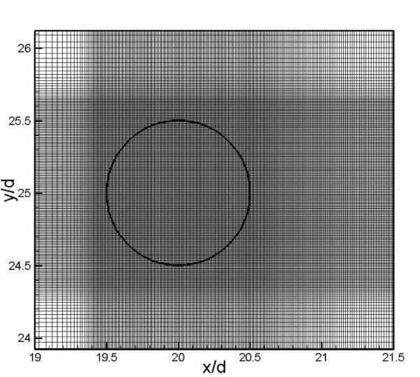
Non-uniform grid employed in the vicinity of the circular cylinder for the Red = 1000 simulations.
Figure 11 presents spanwise vorticity contour plots for for Red = 300 and 1000 at one time-instant and both plots indicate the presence of Karman vortex shedding. The vortex shedding leads to the development of time-varying drag and lift forces and in Fig. 12 we have plotted the temporal variation of the drag and lift coefficients, defined as and respectively where FD and FL are the drag and lift forces respectively. It can be observed that for Red = 300 the vortex shedding reaches a stationary state at a non-dimensional time tU∞/d of about 70 where as the Red = 1000 case attains this state at a non-dimensional time of about 60.
Fig. 11.

Computed spanwise vorticity contour plots for (a) Red = 300 and (b) 1000 at one time-instant.
Fig. 12.

Computed temporal variation of drag and lift coefficients for the (a) Red = 300 and (b) 1000 cases.
In order to validate the simulations we have computed a number of key quantities including mean drag and base pressure coefficient Cpb, where pressure coefficient at any location is defined as . The vortex shedding Strouhal number St = fd/U∞ where f is the vortex shedding frequency has also been computed from the temporal variation of the lift coefficient. All of these flow quantities are computed from data accumulated after the flow has reached a stationary state.
Figure 13a shows the variation of Strouhal number with Reynolds number obtained from the current simulations. Also presented are the results from a number of established experimental and numerical studies and we find good agreement between the present study and past numerical studies. The agreement with the experiment of Williamson[49] is also good up to about Red = 200 beyond which the present study as well as other numerical studies deviate from the experiment. This is due to the fact that at these Reynolds numbers, the flow is intrinsically three-dimensional [50,24] and predictions from 2D simulations tend not to match experiments well in this regime.
Fig. 13.

Comparison of computed (a) vortex shedding Strouhal number (St) and (b) computed base suction coefficient (−Cpb with established computational and experimental results.
Figure 13b shows a comparison of the mean base suction pressure coefficient −Cpb compared to past 2D numerical simulations of Henderson [14] and Mittal & Balachandar[26] and experiments of Williamson and Roshko[48]. Note that the simulations of Henderson[14] employed a spectral element method whereas those of Mittal & Balachandar[26] employed a highly accurate spectral collocation method. It is found that the predictions from the current study match these previous numerical studies over the entire range of Reynolds numbers simulations here. As before, the match with experiments is quite good up to about Red = 200 beyond which intrinsic three-dimensional effects in the experiments lead to a significant mismatch.
Finally, in Table 1 we compare the mean drag coefficient predicted by the current solver with some other numerical studies that have conducted 2D simulations of this flow. The Reynolds number range varies from 40 to 100 and comparisons are made with highly accurate spectral element [14] and spectral collocation [26] as well as another sharp interface, immersed boundary solver [22]. In general, we find very good agreement with these other numerical simulations and this further confirms the accuracy of the current solver a relatively wide range of Reynolds numbers.
Table 1.
Comparison of computed mean drag coefficient with results from previous 2D cylinder simulations.
3.3 Flow Past an Airfoil
In addition to circular cylinder simulations, we have also performed 2D simulations of flow past a NACA 0008 airfoil at two different angles-of-attack (α = 0° and 4°) at chord based Reynolds number (Rec) of 2000 and 6000. These configurations have particular relevance for micro-aerial vehicles [31] where Reynolds numbers tend to be in the range from 102 to 104. A nonuniform 926 × 211 Cartesian grid is used in the current simulations and a relatively large domain size of 9c × 12c where c is the chord length of the airfoil is employed. The grid and domain were chosen after a systematic grid refinement and domain dependence study. Figure 14 shows a flow visualization for the Rec = 6000 and α = 4° case and the simulations indicate that the flow separates from the suction side of the airfoil. Figure 15 presents the temporal variation of the drag and lift coefficients. The simulations are run for a relatively large time duration of tU∞/c = 20 at which point the force on the foil reaches a nearly constant value. These lift and drag coefficients are compared with the numerical simulations of Kunz & Kroo [19] which were carried out using conventional body-conformal grid methods. Table 2 compares these quantities and we find that the current methodology provides a reasonably good prediction of these key quantities.
Fig. 14.

Contour plot of spanwise vorticity at one time-instant for the NACA 0008 airfoil at Rec = 6000 and α = 4°.
Fig. 15.

Temporal variation of force coefficients for NACA 0008 airfoil at α = 4° for Rec = 2000 and 6000 (a) Drag coefficient (b) Lift coefficient.
Table 2.
Comparison of computed steady-state lift and drag coefficient values for NACA 0008 airfoil at two angles-of-attack with the results obtained from simulations of Kunz & Kroo[19].
| Rec → | 2000 | 6000 | ||||||
|---|---|---|---|---|---|---|---|---|
| α → | 0° | 4° | 0° | 4° | ||||
| Study ↓ | CD | CL | CD | CL | CD | CL | CD | CL |
| Present | 0.078 | - | 0.081 | 0.273 | 0.044 | - | 0.047 | 0.240 |
| Kunz & Kroo [19] | 0.076 | - | 0.080 | 0.272 | 0.043 | - | 0.047 | 0.234 |
3.4 Flow Past a Sphere
Flow past a stationary sphere is a canonical flow that allows us to test the fidelity of the solver for three-dimensional flows. A number of experimental [6,40,34], and numerical studies[27,15,28] have examined this flow at low to moderate Reynolds numbers which are accessible via direct numerical simulation. Flow past a sphere is axisymmetric and steady below a Reynolds number (based on the diameter) of 210 [32]. Between Reynolds numbers of 210 and about 280, the flow is non-axisymmetric but steady and beyond that the flow is non-axisymmetric and unsteady.
In the current study we have performed simulations of flow past a stationary sphere with Reynolds numbers ranging from 100 to 350 and made qualitative as well as quantitative comparisons with established data. The Cartesian grids employed have up to 192×120×120 grid points and are non-uniform with grid clustering provided around the sphere and in the near wake. For Red = 100 and 150 the computed flow is steady and axisymmetric and Figure 16a shows the streamline pattern on one plane of symmetry for Red = 100. For these axisymmetric flows, we can identify the center (coordinates (xc, yc)) of the flow recirculation pattern in the wake of the sphere. In Figure 16a this location is denoted by a small white circle. We can also determine the length of the recirculation zone from the back of the sphere denoted by Lb. The values of these parameters for Red = 40 and 150 are compared with previous studies in Table 3 and found to be very much inline with these previous studies.
Fig. 16.

(a) Computed streamline pattern on one plane of symmetry for Red = 100 sphere case. (b) Isosurface of enstrophy at one time-instance for Red = 350 sphere case.
Table 3.
Comparison of key computed results for flow past a sphere with other established experimental and computational studies.
| Red → | 100 | 150 | 300 | 350 | ||||
|---|---|---|---|---|---|---|---|---|
| Study ↓ | xc/d | yc/d | Lb/d | xc/d | yc/d | Lb/d | St | St |
| Mittal[27] | - | - | 0.87 | - | - | - | - | 0.14 |
| Bagchi et al.[1] | - | - | 0.87 | - | - | - | - | 0.135 |
| Johnson & Patel[15] | 0.75 | 0.29 | 0.88 | 0.32 | 0.29 | 1.2 | 0.137 | - |
| Taneda[42] | 0.745 | 0.28 | 0.8 | 0.32 | 0.29 | 1.2 | - | - |
| Marella et al.[22] | - | - | 0.88 | - | - | 1.19 | 0.133 | - |
| Present | 0.742 | 0.278 | 0.84 | 0.31 | 0.3 | 1.17 | 0.135 | 0.142 |
For Red = 300 and 350, the flow is non-axisymmetric and unsteady and Fig. 16b shows a visualization of the enstrophy fields for Red = 350. As has been seen in past studies, the wake at these Reynolds numbers is found to be dominated by vortex loops which exhibit a planar symmetric topology[27]. These simulations are run for a long enough time period so as to reach a well established stationary state. Average quantities such mean force coefficients and vortex shedding Strouhal number are computed based on stationary state data. Figure 17a shows the temporal variation of the drag and side force coefficient for Red = 350 case and these flow quantities clearly show that the flow has reached a stationary state. In Fig. 17b we compare the computed mean drag coefficient with a number of previous experimental and numerical studies and find that the values match quite well with these past studies as well as the correlation of Clift et al.[6]. The temporal variation of pressure in the wake has been used to estimate a vortex shedding Strouhal number and as can be seen in Table 3, this quantity also matches well with past studies.
Fig. 17.

(a) Temporal variation of drag and side force coefficients on a sphere in a uniform flow for Red = 350. (b) Comparison of computed mean drag coefficient with experimental and numerical data.
3.5 Simulation of Flow Past Suddenly Accelerated Bodies
All of the cases simulated so far have been with stationary immersed boundaries. In the current section we describe simulations of flow past moving bodies with the objective of demonstrating the fidelity and accuracy of the current solver for such flows. The focus is on bodies which instantaneously accelerate from zero to a finite velocity Uo in a stagnant fluid. Accurate prediction of the temporal variation of the drag force and wake evolution requires that the thin vorticity layer that develops on the accelerating body be adequately resolved in time and space. Therefore, such flows offer a severe test of both the spatial and temporal accuracy of the method for moving boundaries.
3.5.1 Suddenly Accelerated Normal Plate
This first case of a moving immersed boundary is of an infinitesimally thin finite flat plate of height h accelerating normal to its surface. The Reynolds numbers based Reh = Uoh/ν is chosen to be 126 and 1000 in order to match the simulations of Koumoutsakos & Sheils [18]. These authors employed a vortex particle method for simulating this flow which is particularly well suited for such flows since at least for early times, the vorticity is confined to a small subregion of the domain thereby easing the computational requirements for the simulations. Figure 18 shows the evolution of the separation bubble behind the plate at four different time-steps and these plots compare well with the corresponding Figs. 5 and 8 in the paper of Koumotsakos & Sheils[18]. Figure 19 shows the temporal variation of the computed bubble length (which is the length of the region of reverse flow on the centerline behind the plate normalized by plate height) obtained from the current simulations. Also included in the plot are results from the experiments of Taneda & Honji [43] and simulations of Koumoutsakos & Shiels [18] and we find an excellent match between the three data sets. Note also that this case demonstrates the ability of the solver to handle infinitesimally thin (membraneous) bodies. Membraneous entities such as insect wings and fish fins abound in biology. Infinitesimally thin interfaces are also encountered in flows involving bubbles and drops and therefore, the ability to handle such geometries significantly enhances the operational envelope of the solver. The key issue in dealing with such boundaries is to allow for ghost-cells on both sides of the immersed boundary. Furthermore for such cases, a given ghost-node is also concurrently a fluid-node. In the current solver we have handled this through the use of auxiliary arrays that store ghost-cell nodal values separately from fluid values at a given ghost-cell. Pointers are used to access this auxiliary storage thereby simplifying the solution algorithm for such bodies.
Fig. 18.

Computed spanwise vorticity contours for a suddenly started normal flat-plate at four stages in the start-up process. Upper and lower halves of each figure correspond to Reh = 126 and 1000 respectively. (a) tUo/h = 0.5 (b) 1 (c) 2 and (d) 3.
Fig. 19.

Time evolution of computed bubble length behind flat plate at Reh = 126 and 1000 compared to established experimental and computational results.
3.5.2 Suddenly Accelerated Circular Cylinder
Next we present results of simulated flow past suddenly accelerated circular cylinder. Flow is simulated at two different Reynolds numbers (Red = Uod/v) of 550 and 1000, both of which have been simulated using a vortex particle method by Koumoutsakos & Leonard[17]. The current simulations employ dense 541 × 161 grids in order to resolve the extremely thin boundary layers that develop on the cylinder surface. Figure 20 shows four stages in the evolution of the vortex behind the cylinder at the two Reynolds numbers. These figures compare well with corresponding figures in the paper of Koumoutsakos & Leonard[17]. In Fig. 21 we have plotted the temporal variation of the computed drag coefficient along with available results from [17] for both cases. It is noted that the current immersed boundary calculations match the results of these previous calculations very well, thereby providing further confidence in the ability of the solver to simulate accurately the production and subsequent convection of vorticity from moving and rapidly accelerating bodies bodies as well as the transient fluid-dynamic forces.
Fig. 20.

Computed spanwise vorticity contours for a suddenly started cylinder at four stages in the start-up process. Upper and lower halves of each figure correspond to Reh = 1000 and 550 respectively. (a) tUo/d = 0.5 (b) 1 (c) 1.5 and (d) 2.
Fig. 21.

Time evolution of computed drag coefficient for suddenly started cylinder at Red = 550 and 1000 compared to established experimental and computational results. Also included in the figure is the temporal variation of drag-coefficient for a suddenly started sphere at Red = 550.
Also included in Fig. 21 is the temporal variation of force on a suddenly accelerated sphere at a Reynolds number of 550. For this simulation, we have employed a 541 × 161 × 161 grid which is based on the grid used for the Red = 550 suddenly accelerated cylinder. Although there is no other computational or numerical data available for comparison, we provide this data so that it may be used as a benchmark for moving 3D bodies in the future.
3.6 Simulation of Flow Past Complex Moving Bodies
With the solver validated systematically for two- and three-dimensional stationary and moving boundaries, we now turn to demonstrating the ability of the current solver to simulate flow with highly complex boundaries.
3.6.1 Fish Pectoral Fin Hydrodynamics
The first case chosen is that of a fish pectoral fin. The particular fish which is the subject of this study is the bluegill sunfish, which has been studied extensively by Lauder and co-workers [20,30]. This fish was videotaped swimming steadily in a current of water moving at a speed of about one body-length per second. In this particular swimming mode, the fish uses only its pectoral fins to produce propulsive force and is therefore a good case to study pectoral fin based (“labriform”) propulsion. Two high-speed, high-resolution video cameras are used simultaneously to record the motion of the fin and the videos are used to construct an accurate, three-dimensional, time-varying reconstruction of the fin kinematics. The fin is a thin membranous structure supported by slender bony rays and can therefore be modeled as a membrane in the simulations. The fin position at three stages in the stroke is shown in Fig. 22 and it can be seen that the fin undergoes significant deformation, both active as well as flow-induced as it moves through the fluid. All of this deformation is captured in the videos and incorporated with high fidelity into the reconstructed fin kinematics. The stroke frequency of the fin is about 2Hz and using the length of the longest ray which is 4cm as the length scale and the freestream velocity of 0.16 m/s as the velocity scale, we estimate the Reynolds numbers (Re = U∞LS/v where LS the the spanwise size of the fin) and Strouhal numbers (St = fLS/U∞ where f is the stroke frequency) for this flow to be approximately 6300 and 0.54 respectively. In addition to the fin kinematics, these non-dimensional parameters are also matched in the simulation. Simulations are carried out on two different grids, one with about 2.78 million grid points and the other with about 6 million grid points and here we present results from the larger grid. Simulations are run for over four fin strokes and the results presented are for the fourth stroke. Figure 23 shows a sequence of flow visualizations at three stages in the fin stroke. The fish body is shown for reference purposes only and is not actually included in the simulations. Instead, the fin is put next to a flat-plate which is oriented in the x – y plane. The plot shows streamlines as well as isosurface plots of the imaginary part of the complex eigenvalue of the velocity deformation tensor[41] denoted by Λi. The plots show the formation of a complex system of distinct vortices including a strong abduction tip-vortex from the fin. As this vortex system convects downstream it coalesces into a nearly spherical agglomeration of vortex structures. An ongoing study is examining the thrust production, energetics and associated flow mechanism and a parameter survey of this flow is also being undertaken. Results from this study will be presented in a future publication.
Fig. 22.

Grid employed in the pectoral fin simulations and fin configuration at three stages in its motion.
Fig. 23.

Isosurfaces of ∧i and corresponding streamlines at three stages in the pectoral fin stroke of the bluegill sunfish. (a) t × f = 1/3 (b) t × f = 2/3 (c) t × f = 1. Body of the sunfish is shown for reference only and not included in the simulations.
3.6.2 Dragonfly Flight Aerodynamics
In this section, we present results from a simulation devised to examine aerodynamics of dragonfly flight with a significant level of complexity and realism including the role of wing-wing interaction and wing-body interaction. The results presented here are primarily intended to show the complexity of the flow for such a configuration and the ability of the solver to handle a case which includes a combination of multiple moving/stationary membranes and solid bodies. The dragonfly body and wing anatomy is based on images of a variegated meadowhawk (Sympetrum corruptum) which is a medium-sized dragonfly. Figure 24a shows the final body configuration as well as the surface mesh for dragonfly model which consists of 8832 triangular elements. A Cartesian grid of size 161 × 177 × 113 is used which provides high resolution around the dragonfly and the wake as shown in Fig. 24b. Actual kinematics of dragon-flies in free-flight including, rolling amplitude, pitch angles, inclination of wing stroke-planes, wing beat frequency and phase-relation between the fore- and hind-wings, is available from a number of sources[33,47]. In the current model, we choose a relatively simple representation of the wing kinematics wherein each pair of wings undergoes a sinusoidal pitching-rolling motion where the roll axis is situated at the inner (closer to body) tip of the wing and the pitching is along a spanwise axis located at 10% wing chord. Furthermore, pitching leads the rolling motion by 90° in phase and the forewings also lead the hindwings by 180° in phase. In the specific case presented here, the Reynolds number (Re = U∞c/v) based on the maximum chord length of the fore-wing is 320 and Strouhal number (defined as St = Af/U∞ where A is the peak-to-peak amplitude of the tip of the forewing, and f is the wing flapping frequency) is 0.5. Alias MAYA animation software [8] is used to incorporate the prescribed kinematics into the model and the animation is input into the IBM solver as a sequence of surface velocity files. Figure 25 demonstrates the flow structures of the dragonfly case at three different stages in the flapping cycle. In Figs. 25a and b the two wing pairs are at the extreme positions of their flapping motion and are at the stage of reversing their respective motions. At these stages, the dominant features in the flow are the remnants of the tip and wake vortices created during the stroke. In contrast, Fig. 25c shows the wings at the end of the cycle at which stage both wings are at the center position with the forewings rolling upwards and the hindwings rolling downwards. At this stage, the dominant vortices features in the flow are the detached leading-edge vortices which can be found on the lower(upper) surface of the fore(hind) wings. These vortices are stronger towards the wing-tips where wing velocity is the highest. This dragonfly configuration is being further refined with more realism injected into the wing kinematics from detailed experimental observations [47] and will then be used for a detailed investigation of dragonfly flight aerodynamics.
Fig. 24.

(a) Surface mesh used to define the geometry of the dragonfly body and wings. (b) Two-dimensional view of the dragonfly model immersed in the fluid grid.
Fig. 25.

Isosurfaces of ∧i at three stages in the flapping cycle of a modeled dragonfly. (a) t × f = 0.25 (b) t × f = 0.75 (c) t × f = 1.
4 Conclusions
A highly versatile immersed boundary method for simulating incompressible flow past complex three-dimensional moving boundaries is described. The immersed boundary method is based on a discrete-forcing scheme that allows for a “sharp” representation of the immersed boundary. The immersed boundary method developed is closely coupled with a unstructured grid surface representation of the immersed boundary and salient feature of the IB methodology and the implications of using an unstructured structured mesh are discussed.
A number of diverse two- and three-dimensional canonical flows are simulated and computed results compared with available data sets in order to establish the accuracy and fidelity of the current solver. Reynolds numbers for these flows range from O(101) up to O(103). Simulations are also conducted for flows with moving boundaries and we show that even for rapidly accelerated bodies, the current solver predicts accurately, the temporal variation of the fluid dynamic forces and the evolution of the vorticity field. Finally, we demonstrate the ability of the solver to handle some extremely complicated three-dimensional moving boundaries by showing selected results from a fish-pectoral fin simulation as well as simulation of a dragonfly in flight. These two cases show that the solver can handle complex, highly deformable membranous objects as well as multi-component bodies with membranous as well as non-membranous components in complex relative motion.
Fig. 1.

Schematic describing the naming convention and location of velocity components employed in the spatial discretization of the governing equations.
Acknowledgments
RM would like to acknowledge support for this work from ONR-MURI grant N00014-03-1- 0897, AFOSR Grant F49550-05-1-0169 and NIH Grant R01-DC007125-0181. FM has been supported by the Department of Energy through the University of California under subcontract B523819.
References
- [1].Baghchi P, Ha MY, Balachandar S. Direct numerical simulation of flow and heat transfer from a sphere in a uniform cross flow. J. Fluids Eng. 2001;123:347. [Google Scholar]
- [2].Balaras E. Modeling complex boundaries using an external force field on fixed Cartesian grids in large-eddy simulations. J. Comput. Phys. 2004;33:375. [Google Scholar]
- [3].Bozkurttas M, Dong H, Seshadri V, Mittal R, Najjar F. Towards numerical simulation of flapping foils on fixed Cartesian grids. AIAA Paper 2005-0081. 2005 [Google Scholar]
- [4].Borouchaki H, Lo SH. Fast Delaunay triangulation in three dimensions. Comp. Meth. Appl. Mech. Engr. 1995;128:153–167. [Google Scholar]
- [5].Canann SA, Liu YC, Mobley AV. Automatic 3D Surface Meshing to Address Today's Industrial Needs. Finite Elements Anal. Des. 1997;25:185–198. [Google Scholar]
- [6].Clift R, Grace JR, Weber ME. Bubbles, Drops and Particles. Academic Press; New York: 1978. [Google Scholar]
- [7].Cheng RKC. Inside Rhinoceros 3. Onward Press; 2003. [Google Scholar]
- [8].Derakhshani D. Introducing Maya 8: 3D for Beginners. Maya Press; 2006. [Google Scholar]
- [9].Fadlun EA, Verzicco R, Orlandi P, Mohd-Yusof J. Combined immersed boundary finite-difference methods for three-dimensional complex flow simulations. J. Comput. Phys. 2000;161:30. [Google Scholar]
- [10].Ghias R, Mittal R, Lund TS. A non-body conformal grid method for simulation of compressible flows with complex immersed boundaries. AIAA Paper 2004-0080. 2004 [Google Scholar]
- [11].Ghias R, Mittal R, Dong H. A sharp interface immersed boundary method for viscous compressible flows. J. Comput. Phys. 2007 doi: 10.1016/j.jcp.2008.01.028. To appear in. [DOI] [PMC free article] [PubMed] [Google Scholar]
- [12].Gibou F, Fedkiw RJ, Cheng LT, Kang M. A second-order-accurate symmetric discretization of the Poisson equation on irregular domains. J. Comput. Phys. 2002;176:205. [Google Scholar]
- [13].Goldstein D, Handler R, Sirovich L. Modeling an no-slip flow boundary with an external force field. J. Comput. Phys. 1993;105:354. [Google Scholar]
- [14].Henderson RD. Details of the drag curve near the onset of vortex shedding. Phys. Fluids. 1995;7(9):2102. [Google Scholar]
- [15].Johnson TA, Patel VC. Flow past a sphere up to a Reynolds number of 300. J. Fluid Mech. 1999;378:19. [Google Scholar]
- [16].Kim J, Kim D, Choi H. An immersed boundary finite-volume method for simulations of flows in complex geometries. J. Comput. Phys. 2001;171:132. [Google Scholar]
- [17].Koumoutsakos P, Leonard A. High-resolution simulations of the flow around an impulsively started cylinder using vortex methods. J. Fluid Mech. 1995;296:1. [Google Scholar]
- [18].Koumoutsakos P, Shiels D. Simulations of the viscous flow normal to an impulsively started and uniformly accelerated flat plate. J. Fluid Mech. 1996;328:177. [Google Scholar]
- [19].Knuz PJ, Kroo H. Analysis and Design of Airfoils for use at Ultra-low Reynolds Numbers. In: Mueller TJ, editor. Progress in Astronautics and Aeronautics. 2001. p. 35. [Google Scholar]
- [20].Lauder GV, Madden P, Mittal R, Dong H, Bozkurttas M. Locomotion with flexible propulsors: I. Experimental analysis of pectoral fin swimming in sunfish. Bioinsp. Biomim. 2006;1:25. doi: 10.1088/1748-3182/1/4/S04. [DOI] [PubMed] [Google Scholar]
- [21].Majumdar S, Iaccarino G, Durbin PA. RANS Solver with Adaptive Structured Boundary Non-conforming Grids. Cent. Turbul. Res. Annu. Res. Briefs. 2001:353. [Google Scholar]
- [22].Marella S, Krishnan S, Liu H, Udaykumar HS. Sharp interface Cartesian grid method I: An easily implemented technique for 3D moving boundary computations. J. Comput. Phys. 2005;210:1. [Google Scholar]
- [23].Mavriplis DJ. An advancing front Delaunay triangulation algorithm designed for robustness. J. Comput. Phys. 1995;117:1, 90–101. [Google Scholar]
- [24].Mittal R, Balachandar S. Effect of three-dimensionality on the lift and drag of nominally two-dimensional cylinder. Phys. Fluids. 1995;7(8):1841. [Google Scholar]
- [25].Mittal R, Balachandar S. On the inclusion of three-dimensional effects in simulations of two-dimensional bluff-body wake flows. Symposium on Separated and Complex flows, ASME Summer meeting; Vancouver. 1997. [Google Scholar]
- [26].Mittal R, Moin P. Suitibility of upwind biased schemes for large-eddy simulation of turbulent flows. AIAA J. 1997;35(8):1415. [Google Scholar]
- [27].Mittal R. A Fourier-Chebyshev spectral collacotion method for simulating flow past spheres and spheroids. Int. J. Numer. Meth. Fluids. 1999;30:921. [Google Scholar]
- [28].Mittal R, Wilson JJ, Najjar FM. Symmetry properties of the transitional sphere wake. AIAA Journal. 2002;40(3):579. [Google Scholar]
- [29].Mittal R, Iaccarino G. Immersed boundary methods. Ann. Rev. Fluid Mech. 2005;37:239. [Google Scholar]
- [30].Mittal R, Dong H, Bozkurttas M, Lauder GV, Madden P. Locomotion with flexible propulsors: II. Computational modeling of pectoral fin swimming in sunfish. Bioinsp. Biomim. 2006;1:35. doi: 10.1088/1748-3182/1/4/S05. [DOI] [PubMed] [Google Scholar]
- [31].Mueller TJ, DeLaurier JD. Aerodynamics of small vehicles. Ann. Rev. Fluid Mech. 2003;35:89. [Google Scholar]
- [32].Natarajan R, Acrivos A. The instability of the steady flow past spheres and disks. J. Fluid Mech. 1993;254:323. [Google Scholar]
- [33].Norberg RA. Hovering flight of the dragonfly Aeschna juncea L., kinematics and aerodynamics. In: Wu TY, Brokaw CJ, Brennen C, editors. Swimming and Flying in Nature. Plenum Press; NewYork: 1975. p. 763. [Google Scholar]
- [34].Ormieres D, Provansal M. Transition to turbulence in the wake of a sphere. Phys. Rev. Lett. 1999;83(1):80. [Google Scholar]
- [35].Osher S, Fedkiw RP. Level Set Methods - An Overview and some recent results. J. Comp. Phys. 2001;169:463. [Google Scholar]
- [36].Peskin CS. Flow patterns around the heart valves. J. Comput. Phys. 1972;10:252. [Google Scholar]
- [37].Piegl L. On NURBS: A Survey. IEEE Computer Graphics and Applications. 1991;11:55. [Google Scholar]
- [38].Press WH, Flannery BP, Teukolsky SA, Vetterling WT. Numerical Recipes in Fortran. Cambridge University Press; 1992. [Google Scholar]
- [39].Saiki EM, Biringen S. Numerical simulation of a cylinder in uniform flow: application of a virtual boundary method. J. Comput. Phys. 1996;123:450. [Google Scholar]
- [40].Sakamoto H, Haniu H. The formation mechanism and shedding frequency of vortices from a sphere in uniform shear flow. J. Fluid Mech. 1995;287:151. [Google Scholar]
- [41].Soria J, Cantwell BJ. Identification and classification of topological structures in free shear flows. In: Bonnet JP, Glauser MN, editors. Eddy Structure Identification in Free Turbulent Shear Flows. Kluwer Academic Publishers; Netherlands: [Google Scholar]
- [42].Taneda S. Experimental investigation of the wake behind a sphere at low Reynolds numbers. J. Phys. Soc. Japan. 1956;11(10):1104. [Google Scholar]
- [43].Taneda S, Honji H. Unsteady flow past a flat plate normal to the direction of motion. J. Phys. Soc. Japan. 1971;30(1):262. [Google Scholar]
- [44].Udaykumar HS, Mittal R, Shyy W. Computational of solid-liquid phase fronts in the sharp interface limit on fixed grids. J. Comput. Phys. 1999;153:535. [Google Scholar]
- [45].Udaykumar HS, Mittal R, Rampunggoon P, Khanna A. A sharp interface Cartesian grid method for simulating flows with complex moving boundaries. J. Comput. Phys. 2001;174:345. [Google Scholar]
- [46].Van Kan J. A second-order accurate pressure-correction scheme for vicous incompressible flow. SIAM J. Sci. Stat. Comput. 1986;7:870. [Google Scholar]
- [47].Wakeling JM, Ellington CP. Dragonfly flight, (2). velocities, accelerations and kinematics of flapping flight. J. Exp. Biol. 1997;200:557. doi: 10.1242/jeb.200.3.557. [DOI] [PubMed] [Google Scholar]
- [48].Williamson CHK, Roshko A. Measurment of base pressure in the wake of a cylinder at low Raynolds numbers. Z. Flugwiss. Weltraumforsch. 1990;14:38. [Google Scholar]
- [49].Williamson CHK. The natural and forced formation of spot-like' vortex dislocations' in the transition of a wake. J. Fluid Mech. 1992;243:393. [Google Scholar]
- [50].Williamson CHK. Vortex dynamics in the cylinder wake. Ann. Rev. Fluid Mech. 1996;8:477. [Google Scholar]
- [51].Ye T, Mittal R, Udaykumar HS, Shyy W. An accurate Cartesian grid method for viscous incompressible flows with complex immersed boundaries. J. Comput. Phys. 1999;156:209. [Google Scholar]
- [52].You D, Wang M, Mittal R, Moin P. Study of rotor tip-clearance flow using large eddy simulation. AIAA Paper 2003-0838. 2003 [Google Scholar]
- [53].Zang Y, Streett RL, Koseff JR. A non-staggered fractional step method for time-dependent incompressible Navier-Stokes equations in curvilinear coordinates. J. Comp. Phys. 1994;114:18. [Google Scholar]
- [54].Zhang HQ, Fey Y, Noack BR. On the transition of the cylinder wake. Phys. Fluids. 1995;7(4):779. [Google Scholar]