Manipulation of Conformational Change in Proteins by Single-Residue Perturbations

Abstract

Using the perturbation-response scanning (PRS) technique, we study a set of 25 proteins that display a variety of conformational motions upon ligand binding (e.g., shear, hinge, allosteric). In most cases, PRS determines single residues that may be manipulated to achieve the resulting conformational change. PRS reveals that for some proteins, binding-induced conformational change may be achieved through the perturbation of residues scattered throughout the protein, whereas in others, perturbation of specific residues confined to a highly specific region is necessary. Overlaps between the experimental and PRS-calculated atomic displacement vectors are usually more descriptive of the conformational change than those obtained from a modal analysis of elastic network models. Furthermore, the largest overlaps obtained by the latter approach do not always appear in the most collective modes; there are cases where more than one mode yields comparable overlap sizes. We show that success of the modal analysis depends on an absence of redundant paths in the protein. PRS thus demonstrates that several relevant modes can be induced simultaneously by perturbing a single select residue on the protein. We also illustrate the biological relevance of applying PRS to the GroEL, adenylate kinase, myosin, and kinesin structures in detail by showing that the residues whose perturbation leads to precise conformational changes usually correspond to those experimentally determined to be functionally important.

Introduction

A comparison of the experimentally determined apo and holo forms of a protein provides a wealth of information on the basic motions involved in binding of the ligand, as well as the residues participating in functionality. Such knowledge base is extremely important for deciphering key residues that may be targeted for drug design purposes, or enhancing enzymatic activity. Computational techniques have been developed to distill information from the structures, going beyond the original studies that relied on their visual inspection. Normal mode analysis, in particular, turned out to be a useful technique in the analysis of functionally related conformational dynamics (1,2). As such, it has made possible the classification of protein motions, e.g., hinge bending and shear (3). It has further been shown that the predominant contributions to these motions may be described by a single, most collective mode for some proteins, whereas it may be obtained from a superposition of several modes for others (4). With the advent of coarse graining of biomolecular structures through residue-based network models (3,5–9), it has been possible to study a large number of protein structures. These anisotropic network models (ANMs) take into account the three-dimensional geometry of interacting pairs of residues to study the modal behavior of proteins. Using such information, it is possible to morph between the apo and holo structures to gain insight into the intermediates that lead to the final structure (10–16). These analyses also uncover the different modes stimulated by different ligands binding to the same apo form. Moreover, displacement vectors obtained from the modes might be used to generate alternative starting structures for molecular dynamics (MD) simulations, or to make educated guesses for missing residues in the experimentally determined structures (17). In addition, docking algorithms are improved by incorporating the flexibility of the receptor in the calculations through normal mode predictions (18,19).

Although there is considerable success in these classifications, there is also a debate on, and lack of insight into, how these modes are utilized originally by different types of proteins, or by different ligands acting on the same protein. This problem has been addressed by a methodology that assesses the number of modes necessary to map a given conformational change (17). Therein, the degree of accuracy obtained from the inclusion of a given number of modes was shown to be protein-dependent. In another study where 170 pairs of structures were systematically analyzed, it was shown that the success of coarse-grained elastic network models may be improved by recognizing the rigidity of some residue clusters (20). The studies showed that the collectivity of the motion is detrimental to the ability to represent the motion by a few slow modes.

Notwithstanding its success in identifying the types of motions involved in ligand binding, ANM is an equilibrium methodology, providing information on the equilibrium fluctuations and the various contributions to those fluctuations from different modes of motion. Similar to experimental procedures that lead to useful information, it is of interest to devise a methodology where a perturbation is inserted into the system to place the structure slightly out of equilibrium. The response is recorded to detect the underlying features contributing to the observations, yielding valuable information beyond the correlations between the fluctuations inherent in the system at equilibrium.

A perturbation-response technique applied to the all-atom model of the protein was used to elucidate the shifts in the energy landscape that accompany binding (21). Using that technique, the perturbations are introduced as local displacements of selected atoms followed by energy minimization; the response is then measured as the relative ability of a residue to induce displacements of other residues versus its propensity to resist change. This molecular-mechanics-based methodology relies on scanning all the residues to produce comparative results. In another near-equilibrium methodology, this time applied to the coarse-grained network structure of a protein, one can insert forces into the contact between a chosen pair of residues and uncover the control mechanism that adaptively annihilates the induced change (22). Similar approaches have been adopted in other work, where the perturbations on residues are introduced by modifying the effective force constants (23), distances between contacting pairs (16,24), or both (25). Conversely, one may insert the forces on the nodes instead of on the links between pairs of nodes; depending on the location of the perturbation, the resulting displacements between the apo and holo forms may be highly correlated with those determined experimentally (26). Recently, this approach was extended to scan the whole protein residue by residue, a methodology termed perturbation-response scanning (PRS) (27). By recording the response to each inserted force on the ferric binding protein (FBP), it has been possible to map those residues that are structurally amenable to inducing the necessary conformational change upon binding. Moreover, independent of the directionality of the inserted force in a remotely located residue, the directionality of the response is found to be organized around the binding region of FBP. The strength of all the above-mentioned techniques is that they recognize the contributions to the motions from all degrees of freedom of the system, rather than focusing on a subset represented by a few slow normal modes. These methods are able to bring out an underlying feature of the system by observing the response to a disturbance of the system slightly out of equilibrium, within the linear-response regime.

We study 25 pairs of structures using PRS and ANM. We show that PRS maps residues that may alone manipulate the structure between the apo and holo forms during ligand binding. With ANM, we determine the mode whose base vector best reproduces the motion between the two forms for each protein pair. We show that in all the cases inspected, manipulation of a single residue will reproduce the structural change more effectively than that of the best mode in ANM. The variability of the number and location of the residues that reproduce the displacement profile yields clues to how that particular protein functions, as shown by case studies.

Methods

Theory

Here, we present a review of how a native protein structure may be manipulated by external forces (27). We assemble the folded protein as a network of N nodes on the C_α atoms. Any given pair of nodes interacts in accord with a conventional harmonic potential, if the nodes are within a cut-off distance, R_c, of each other.

In the notation used, r and f are the bond and internal force vectors along the edge connecting any two nodes, respectively. On the other hand, R and F are vectors on the nodes and are called the position and external force vectors, respectively. There are m_i interactions for each residue i (e.g., if residue 11 has four interactions, m₁₁ = 4), and a total of M interactions for N residues (i.e., M = Σm_i/2). In the absence of external force acting on the system, the equilibrium condition for each residue i requires that the summation of the internal residue-residue interaction forces must be zero for each residue:

$$\mathbf{b}\Delta {\mathbf{f}}_i=0,$$ (1)

where the 3 × m_i coefficient matrix b consists of the direction cosines of each force representing the residue-residue interaction. The row indices of b are x, y, or z. Here, Δf_i is an m × 1 column matrix of forces aligned in the direction of the bond between the two interacting residues. For instance, if a residue i has nine contacts, Δf_i is a 9 × 1 column matrix. Following the numerical example, Eq. 1 sums up the projection of these nine forces on the x, y, and z axes.

One can write the equilibrium condition (Eq. 1) for each residue. This leads to a total of N sets of equations, each of which involves the summation of forces in three respective directions. Generalizing Eq. 1 to the whole system of N residues and M interactions, one can write an algebraic system of a total of 3N equations consisting of M unknown residue-residue interaction forces:

$$\mathbf{B}\Delta {\mathbf{f}}_i=0,$$ (2)

with the 3N × M direction cosine matrix B and the M × 1 column matrix of residue-residue interaction forces, Δf. It is straightforward to generate the matrix B from the topology of the native structure (i.e., the protein data bank (PDB) file (28)) with a specified r_c. As an example, formate dehydrogenase (FD) has 374 residues and a total of 1816 interactions when R_c = 8.0 Å is selected.

In the presence of an external force, ΔF, the equilibrium condition for each residue imposes that the summation of the residue-residue interaction forces must be equal to the external applied force on the same residue. Then, Eq. 2 may be expressed as

$${\mathbf{B}}_{3N\times M}\Delta {\mathbf{f}}_{M\times 1}=\Delta {\mathbf{F}}_{3N\times 1}.$$ (3)

Under the action of external forces, each residue experiences a displacement, ΔR, which is the positional displacement vector. Moreover, the bond distance between any two residues changes by Δr in accord with the positional displacements of two residues that participate in the contact. Therefore, there must be compatibility between the 3N positional displacements and the changes that take place in the intraresidual distances, a total of M distortions. This compatibility is very similar to the form given in Eq. 3 (22):

$${\mathbf{B}}_{M\times 3N}^{\text{T}}\Delta {\mathbf{R}}_{3N\times 1}=\Delta {\mathbf{r}}_{M\times 1}.$$ (4)

Within the scope of an elastic network of residues that are connected to their neighbors by linear-elastic springs, the residual interaction forces, Δf, are related to the changes in the contact distances, Δr, through Hooke's law by

$${\mathbf{K}}_{M\times M}\Delta {\mathbf{r}}_{M\times 1}=\Delta {\mathbf{f}}_{M\times 1},$$ (5)

where the coefficient matrix K is diagonal. We take the entries of K to be equivalent. We have previously validated this assumption by comparing residue cross-correlations obtained from the simplified Hookean potential in Eq. 5 with those from MD simulations (21,27,29).

Thus, rearranging Eqs 3–5, one gets the forces necessary to induce a given point-by-point displacement of residues:

$$\left(\mathbf{B}\mathbf{K}{\mathbf{B}}^{\mathbf{T}}\right)\Delta \mathbf{R}=\Delta \mathbf{F}$$ (6)

On the other hand, one may choose to perturb a single residue or a set of residues, and follow the response of the residue network through

$${\left(\mathbf{B}\mathbf{K}{\mathbf{B}}^{\mathbf{T}}\right)}^{-1}\Delta \mathbf{F}=\Delta \mathbf{R},$$ (7)

where the ΔF vector will contain the components of the externally applied force vectors on the selected residues.

Perturbation-response scanning

We analyze a set of 25 proteins in their apo and holo forms (Table 1). Unless otherwise specified, for each pair of experimental structures, the holo is superimposed on the apo form, followed by the computation of the residue displacement vectors, ΔD. In PRS, we perturb the apo form of each protein by applying a random force to the C_α atom of a residue. We scan the protein, consecutively perturbing each residue i by applying the force ΔF. Thus, the elements of the ΔF vector are nonzero only for the three terms ΔF_3i−2, ΔF_3i−1, and ΔF_3i. We then record the expected changes, ΔR, as a result of the linear response of the protein, computed through Eq. 7. We report the averages over 10 independent runs where the forces are applied randomly within a sphere by simultaneously applying forces in the x-, y-, z-directions with the magnitudes chosen uniformly in the interval (−0.1, 0.1). One realization of PRS on the largest system studied, topoisomerase II (TII), with M = 8877 interactions, takes 30 min time on Intel Xeon 2.70 GHz CPU. The smallest systems take ∼10 s to analyze.

Table 1.

Results for proteins studied by PRS and ANM

	Protein	apo/holo∗	Type of motion†	N‡	RMSD (Å)§	Rcopt (Å) (PRS/ANM)¶	PRS overlap (average/best)‖	ANM overlap (mode No.)∗∗	Mode classification††
Subdomain motions	Thymidylate Synthase	3tms/2tsc	Shear	264	0.80	8.6/9.0	0.59(12)/0.71	0.60 (1)	I
	Tetracycline repressor (TR)	1bjz/1bjy	Shear	179	0.83	12.1/11.0	0.21(9)/0.29	0.37 (16)	III
	Small G protein Arf6	1e0s/2j5x	Shear	164	4.17	13.0/13.0	0.29(14)/0.42	0.37 (12)	III
	Annexin V	1anx/1avr	Hinge	316	1.77	8.3/8.9	0.35(5)/0.49	0.31 (1)	II
	FecA transporter	1kmo/1kmp	Hinge	647	1.79	9.2/9.4	0.40(11)/0.54	0.37 (15)	III
	OxyR transcription factor(OTF)	1i6a/1i69	not hinge or Shear	206	2.05	9.2/10.5	0.23(12)/0.37	0.25 (5)	III
	Ubiquitin conj. enzyme (UCE)	1j74/1j7d	not hinge or Shear	139	1.93	9.6/9.0	0.52(12)/0.62	0.55 (2)	I
Domain motions	Cytochrome P450BM-3	1bu7/1jpz	Shear	453	1.13	7.9/8.2	0.43(9)/0.58	0.48 (4)	I
	Molybdate-binding prot.	1h9k/1h9m	Shear	141	0.87	11.8/11.9	0.45(14)/0.64	0.62 (3)	II
	Kinesin	1i5s/1vfw	Shear	317	1.99	9.5/9.5	0.28(10)/0.43	0.31 (13)	III
	Adenylate Kinase (ADK)	4ake/1ake	Hinge	214	7.13	9.0/8.0	0.82(3)/0.93	0.80 (1)	I
	Formate Dehydrogenase (FD)	2nac/2nad	Hinge	374	1.18	8.0/8.0	0.72(13)/0.92	0.68 (3)	I
	Ferric binding protein (FBP)	1d9v/1mrp	Hinge	309	2.48	7.9/8.0	0.86(10)/0.94	0.94 (1)	I
	Maltose binding protein (MBP)	1omp/3mbp	Hinge	370	3.65	8.7/7.9	0.85(6)/0.95	0.83 (2)	I
	Myosin	1vom/2aka	Not fully classified	730	6.57	9.5/9.5	0.66(10)/0.78	0.62 (1)	I
	Aldose reductase4	2acq/1mar	Not hinge or shear	315	0.51	10.5/10.4	0.46(20)/0.62	0.50 (1)	II
	Immunoglobulin	1mcp/4fab	Not hinge or shear	214	5.90	7.5/8.0	0.68(2)/0.73	0.65 (1)	I
	HIV-1 Rev. Transcriptase	2hmi/3hvt	Partial refolding	555	3.45	9.5/9.0	0.63(7)/0.76	0.51 (1)	I
	Serpin	1psi/7api	Partial refolding	372	8.60	9.5/9.0	0.30(11)/0.41	0.29 (3)	II
Subunit motions	Hemoglobin	4hhb/2hco	Allosteric	141	0.73	9.3/8.3	0.40(5)/0.54	0.48 (1)	I
	VirB11 ATPase	1g6o/1nlz	Allosteric	323	0.93	9.5/9.5	0.63(14)/0.79	0.67 (3)	I
	Aspartate Receptor (AR)	1lih/2lig	Nonallosteric	157	2.58	9.3/9.5	0.38(11)/0.51	0.37 (1)	II
	MalK	1q12/1q1b	Nonallosteric	367	1.16	8.0/8.0	0.55(9)/0.71	0.60 (2)	I
	GroEL	1aon/1oel	Complex motions	524	12.38	10.0/10.0	0.81(2)/0.88	0.80 (1)	I
	Topoisomerase II (TII)	1bgw/1bjt	Complex motions	664	20.57	12.0/13.0	0.21(8)/0.30	0.41 (7)	III

^∗PDB code.

^†Type of motion is classified according to the Yale Morph server (10).

^‡N refers to the number of residues used in the analyses.

^§Backbone RMSD except in the case of aldose reductase, where the 1mar structure has only the C_α atoms available. RMSD, root-mean-squared deviation.

^¶Optimized cutoff distance, as described in the text.

^‖Highest overlap between the scanned structures in the PRS technique and those in the experimental displacements, reported as the average over 10 runs as well as the single best result obtained from any residue; the standard deviation is reported in parentheses. Bold print is used for O_i > 0.5.

^∗∗Highest overlap between the eigenvectors best representing the conformational change of the apo structure; the corresponding mode index is reported in parentheses.

^††See Methods section for a description of the mode classification process.

To assess the quality of the predicted displacements of all residues resulting from a force applied on selected residue i, we use the overlap of the predicted and experimental displacements:

$$O_i=\frac{{(\Delta \mathbf{R})}^i·\Delta \mathbf{D}}{{\left|{(\Delta \mathbf{R}·\Delta {\mathbf{R}}^{\text{T}})}^i{(\Delta \mathbf{D}·\Delta {\mathbf{D}}^{\text{T}})}^i\right|}^{1/2}}.$$ (8)

A value close to 1 implies good agreement with experiment, and a value of zero indicates a lack of correlation between experiment and theoretical findings.

Modal analysis

Equivalence of the equilibrium fluctuations obtained from the normal modes and the force balance (Eq. 6) was shown in a previous work, wherein the modal decomposition was also performed (5). Thus, (BKB^T) is the 3N × 3N matrix equivalent to the Hessian, H, of the system studied. The pseudoinverse of the H matrix is obtained as H⁻¹ = U Λ⁻¹ U^T, where Λ is a diagonal matrix whose elements, λ_j, are the eigenvalues of H, and U is the orthonormal matrix whose columns, u_j, are the eigenvectors of H. H has at least six zero eigenvalues corresponding to the purely translational and rotational motions. In modal analysis, for a given mode j, u_j are treated as displacement vectors. Overlaps between the 3N elements of the u_j and ΔD vectors are used to select the mode j that best describes the binding motion. To assess the quality of the modes obtained by H⁻¹, we use the overlap equation (Eq. 8) by replacing the displacement vector upon perturbation, ΔR, with the normal vector, u_j.

Furthermore, to emphasize the differences between the modal structures of the proteins, we classify a protein as type I if its conformational change is dominated by collective modes, type III if the conformational change is distributed among many modes, and type II for the intermediate cases. For this purpose, we extensively examine the overlap distributions for every protein for a large range of R_c. We define as type I those proteins that have one or two O_i > 0.4 lying in the first four most collective modes. Proteins are classified as type II if they have their most dominant mode in the first five most collective modes with a value of 0.25 < O_i < 0.60 along with higher indexed modes with O_i values of similar magnitude. The remaining proteins are classified as type III. We find that although the values of the overlaps and the mode indices depend on the choice of R_c, the mode classification is robust toward this choice. The only two exceptions are the small proteins UCE and hemoglobin, whose mode classifications shift from type I to type II at higher R_c values.

Optimization of the cut-off distance

The eigenvalue distribution of the Hessian of proteins is such that the low-frequency region is more crowded than expected of polymers or other condensed matter (30). Thus, the choice of the cutoff distance, R_c, for the construction of the Hessian is critical for extracting proteinlike properties from the systems studied. For all the proteins studied in this work, we coarse-grain the PDB structure so that each residue is represented by the coordinates of its C_α atom. We then repeat the PRS analysis for a variety of cut-off distances in the range of 7.0–14.0 Å in increments of 0.1 Å; the lower limit defines the first coordination shell of residues in proteins. For each network structure, we ensure that the system has six zero eigenvalues corresponding to the translational and rotational degrees of freedom of the protein. For a given protein, we select the cut-off distance, $R_c^{\text{opt}}$, that yields the closest agreement of the displacement vectors from experiments for at least one residue. We verify that the overlap values reported in the Results section are not affected for the range of values $R_c^{\text{opt}}\pm 0.2$ Å for all the 25 proteins studied. We also verify that the order of residue indices that provide the best overlaps does not change within this range of $R_c^{\text{opt}}$. Note that $R_c^{\text{opt}}$ is independent of the size of the protein (Table 1). Optimization is done separately for PRS and ANM. To present the effect of choosing a uniform R_c, we also display the results for a single R_c = 9.5 Å. We choose this value, because it is the smallest common R_c at which we obtain six zero eigenvalues for all the proteins tested, except for topoisomerase where that cutoff is 12 Å.

Redundancy index

In this work, we define a new metric called the redundancy index, which is a measure of the degree of collectivity of motions in a protein. We define a nonbonded contact between a pair of residues p and q as follows: a residue q within the distance R_c of p is not its first or second neighbor along the contour of the chain, i.e., | p – q |≥ 3. We quantify the redundancy in the protein by the number of possible ways to reach a nonbonded contact of a residue if its direct contact were momentarily screened.

We calculate the number of alternative routes from p to its nonbonded contact q through other edges of p in the residue network. Letting t_m,_pq be the number of ways of reaching a direct contact q of residue p in m steps, one first forms the perturbed adjacency matrix, M^pq, from the coordinates of the C_α atoms, whose elements are given by

$$M_{ij}^{pq}=\{\begin{array}{c}H\left(R_c-R_{ij}\right)\\ 0\\ 0\end{array}\begin{array}{c}i\ne j\\ i=j\\ i=p,j=q\end{array},$$ (9)

where R_ij is the distance between residues i and j, H(x) is the Heaviside step function whose value is zero for x ≤ 0, and 1 otherwise. Note that Eq. 9 explicitly states why the matrix M is referred to as perturbed. A selected direct nonbonded contact between the residue p and neighbor q is set to zero. The powers property of the adjacency matrix dictates that its mth power gives the number of m-step paths to reach q from p. Thus, t_m,_pq = (M^pq)^m, and, in particular, the number of two-step paths is given by t_2,pq = (M^pq)².

The calculation is repeated for all nonbonded contact pairs (p, q). For each residue p, the two-step paths to the nonbonded contacting neighbor q are normalized by the total number of such contacts of the pth residue, k_p:

$$t_{2,p}=\frac{{\sum }_{q=1}^N{t}_{2,pq}}{k_p}$$ (10)

The number of redundancies generated by a given residue also depends on the location of the residue in the network, the more central residues having higher reachability. This property is quantified by the average shortest path length, L_i, of the residue, which is highly correlated with the experimentally measured residue fluctuations (31). For each residue i, it is an average value over the minimum number of connections that must be transversed to connect it with its jth neighbor, $L_i=1/N{\sum }_{j=1}^N{L}_{ij}$, computed by the Dijkstra algorithm. Thus, we define the redundancy index, r, of the protein as the ratio of the number of alternative two-step paths a given residue i generates to its nonbonded contacts (a local property) and its overall reachability (a global property):

$$r_i=\frac{t_{2,i}}{L_i}.$$ (11)

In general, one would expect all paths to long-range contacts to be effective on r; i.e., all screened n-step paths, each with t_n,i. However, the two-step paths are expected to have the largest contributions in the fluctuating environment of the protein when direct paths are momentarily screened.

Results

Analysis of proteins with different conformational change classifications

We study the conformational change upon ligand binding of a set of 25 proteins (Table 1) that show various types of motions, such as shear, hinge, allosteric, partial refolding, and more complex motions within subdomains, between subdomains and between subunits of the proteins, as classified in the Yale Morph server (10). For each protein, we perform two analyses. 1), With PRS, we scan the protein by inserting random forces on all residues sequentially. For each residue, we then record the overlap of the response vector with the experimental conformational change vector (O_i; Eq. 8). In Table 1, we report the highest overlap and the standard deviations from m = 10 runs, as well as the single best case obtained. 2), With ANM, we seek the mode that best represents the conformational change. We therefore calculate the overlap of each eigenvector of the Hessian matrix (u_j) with the experimentally determined conformational change between the apo and holo structures (ΔD). The highest overlaps are reported in Table 1 along with the mode number. Note that modes are sequentially numbered from the slowest to the fastest, excluding the six corresponding to the translation and rotation of the protein; i.e., the most collective nontrivial mode is numbered as 1.

We first observe from the PRS results that for 7 of the 25 proteins, the perturbation of a single residue, irrespective of the direction of perturbation, captures the conformational change pattern (O_i > 0.7 for the average over 10 runs, shaded gray in Table 1). These apo and holo structures are linearly connected, although the size of the conformational change may be relatively large (RMSD between the structures is in the range 1.2–12.4 Å). The structures include GroEL, myosin, and immunoglobulin, as well as all four of the proteins displaying hinge motions between their domains, i.e., adenylate kinase (ADK), FD, FBP, and maltose binding protein (MBP). Of these, we will study ADK and GroEL in detail as case studies; myosin results are presented in the Supporting Material. FBP was studied in detail previously using the PRS technique and MD (27). Furthermore, for 19 of the 25 proteins, residue displacements may be captured by singly placed forces on select residues in select directions (O_i > 0.5, shown in print in Table 1). For several cases, O_i > 0.8, implying that it is possible to capture almost the whole conformational change by perturbing a select residue in the correct direction.

It is interesting to note that although many of these proteins display large overlaps, the numbers of residues yielding these large overlaps differ among proteins. For some proteins, there is not much specificity on the residue to be perturbed to reproduce the conformational change. For others, by perturbing a very specific location, the whole conformational change is obtained. The former category is exemplified by FBP: as long as one avoids perturbations on deeply buried residues or those that reside in key locations on secondary structural units, a force exerted on single residues leads to the conformational change (27). In such proteins, the holo form is thought to reside close to the apo form on the free energy surface, as a weakly populated conformation.

Our observations from the ANM analysis seeking a single mode that best represents the conformational change have different qualities. Similar to the PRS analysis, the four proteins that have hinge motions between the domains, along with GroEL, VirB11 ATPase, and immunoglobulin, display high overlaps with the experimentally measured conformational change upon binding (O_i > 0.7). In all these cases, the conformational change is best represented by one of the three slowest modes, and these proteins are classified as type I, where the motion is well described by the few most collective modes.

In other proteins, the mode that gives the best representation of the motion is not one of the most collective in these proteins (e.g., the shear motions between the subdomains of TR motions are reproduced with mode 16 and the complex motions of TII with mode 7); such proteins are classified as type III. In other cases (type II proteins), there are a couple of modes with relatively high overlaps of the same magnitude; one of these modes is among the most collective, whereas the other is not.

In Fig. 1, we display the experimental displacement profiles for four sample proteins, ADK, aspartate receptor (AR), UCE, and FD, and we compare them with the PRS and ANM predictions. We find that PRS captures most of the details recorded in the experimental conformational change; predictions by single modes are less descriptive of the total conformational change. In fact, except for TR and TII, PRS always locates single residues whose perturbation in a specific direction is more descriptive of the overall conformational change than any given mode. Thus, by perturbing specific residues, it is possible to act on multiple modes to induce conformational changes that are functionally relevant. These findings are in accord with those from studies where the success of single ANM modes in predicting conformational change was shown to be highly protein-dependent (17). It has been proposed that such dominance of a single mode is related to the collectivity of the transition (20). In the next subsection we use a metric—the so-called redundancy index—that specifies the degree of such collectivity, hence the dominance of a single mode.

Figure 1.

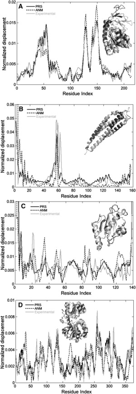
C_α displacement results for (A) ADK, (B) AR, (C) UCE, and (D) FD. Gray line represents the experimental C_α displacements between open and closed structures, black curve is the prediction of PRS, and dashed curve is obtained from the best normal-mode vector in ANM. Area under each curve is normalized to unity. Respective correlations between the experimental conformational change and theoretical binding-induced fluctuation profiles of PRS and ANM are 0.96 and 0.91 for ADK, 0.87 and 0.65 for AR, 0.95 and 0.88 for UCE, and 0.91 and 0.52 for FD. Insets show ribbon diagrams of superimposed proteins, with the open form in black and the closed form in gray.

Redundancy index as a first-order measure of collectivity in the protein

The degree of collectivity of motions in a protein depends on the propensity of its residues to find alternative routes to communicate with function-related destinations such as the active site. Our working hypothesis is that the larger the number of pathways between two regions in the protein, the more complicated the motions within the structure are expected to be. Thus, a superposition of a larger number of collective modes shall lead to those motions. We measure such redundancies created in the protein by the redundancy index, r (Eq. 11).

In Fig. 2 a, we display the relationship between <r_i>, averaged over all the residues, and its variance for the set of 25 proteins shown in Table 1. The points in Fig. 2 A are marked according to the mode classification (Table 1, rightmost column). In general, a high <r_i> leads to mode type III protein (less collective) and a low <r_i> leads to mode type I (most collective). Type II proteins appear as intermediate cases. The Spearman correlation between <r_i> and the mode type is 0.73 (p < 0.0001).

Figure 2.

(A) Average redundancy index versus variance plot for the proteins listed in Table 1, colored according to the mode that best represents the conformational change between the apo and holo forms. Experimental binding-induced conformational change in proteins with low redundancy index (and low variance) are well represented by one of the four slowest modes. (B and C) Probability distribution of redundancy index (B) and average path length versus average redundancy/residue (C) for the residues of ADK and OTF.

Here, the optimal cutoff is different for every protein, because the local packing arrangements are unique to a given protein. To check the effect of choice of R_c, when we reproduce Fig. 2 A using a single value, the correlation is reduced to 0.60 (p = 0.0019) and 0.60 (p = 0.0018) at R_c = 9.5 and 12 Å, respectively (Fig. S2 in the Supporting Material). We also find that the regression line between the average redundancy and standard deviation approaches a perfect line for optimized R_c, whereas it shows larger deviations at fixed values. Thus, in our experience, optimizing the R_c value to reproduce the largest possible overlaps also reproduces the most correlated results, although the main conclusions of the article are not affected by this choice, as long as it is in the range that properly reproduces the eigenvalue distributions representative of proteins (5). Note that the different optimal cutoffs indicate a limitation of elastic network models with a single spring constant. A viable research project would be to utilize different coarse-grained models proposed in the literature, e.g., those of Hinsen (3), Kondrashov et al. (8), and Yang et al. (9), to investigate the implications of this limitation on the methodology presented here.

Proteins with a low <r_i> value also display a narrow distribution, so that most residues have similar redundancy. Such structures are expected to support collective motions, symbolized by a single or a few slow modes. As examples, in Fig. 2 B, we show the distribution of r_i for ADK and OxyR transcription factor (OTF), with similar size. The average for the former is 0.83 ± 0.21 and it is very narrowly distributed. As a consequence, its conformational change is well described by the most collective mode (O_i = 0.80; Table 1). The latter has a wider distribution, with an average value of 3.04 ± 0.97. Its conformational change may not be projected onto a single mode. In general, we find that the more collective mode description of the size of the displacement upon binding, ΔD, corresponds to low values of <r_i> with narrow distributions. Conversely, ΔD values best described by less collective modes are accompanied by poor overlaps (O_i < 0.4).

We also focus on contributions to <r_i> from the local and global structure of the protein; i.e., we compare the number of two-step paths from a residue to its long-range contacts, t_2,i, with its reachability, L_i. These numbers are displayed in Fig. 2 C for ADK and OTF, two proteins of similar size but with different mode classifications. The former has a nonglobular structure, with L_i in the range 4–10. Although the values of L_i cover a large range, they have a positive correlation with t_2,i leading to the narrow distribution of r_i in Fig. 2 B. The behavior observed in OTF has the opposite trends in L_i and t_2,i, leading to a wider distribution of their ratio. Thus, in a given structure, there are both centrally and distantly located residues, but the location need not dictate the number of local alternative connections to the immediate neighbors. It is the balance between these local and global measures that finally determines the collectivity of the motion.

We note that <r_i> is not a perfect measure of the tendency to move collectively, and in many cases, the higher-order contributions neglected in Eq. 11 may explain the discrepancies. Nevertheless, it provides a means to inspect a given protein structure to determine whether the conformational change can be described by a few normal modes. PRS, on the other hand, poses the alternative question, Can all the modes that lead to a given conformational change be invoked by perturbing a single residue? The degree of success presented in Table 1 and Fig. 1 suggests that the answer is affirmative for many of the proteins studied. Our studies further indicate that those residues that lead to high correlation/overlap values hold key locations in the protein structure. We next inspect two of these proteins in detail to demonstrate how PRS may be utilized to determine structurally/functionally important residues.

Case studies illustrating the biological relevance of the PRS method

In this section, we apply the PRS analysis to two proteins, GroEL and ADK. Note that here we perform the PRS analysis on two separate conformations to determine the shift in the roles of residues. Conversely, in Table 1, only the results from open conformations are reported. In addition, results for myosin and kinesin, whose conformational change have been studied in detail using several approaches (16), are presented in Fig. S3, Table S3, and Table S4.

GroEL

GroEL, a molecular chaperone, helps in the folding of substrate proteins that might otherwise aggregate. It uses ATP as the energy source; thus, binding of ATP to GroEL initiates the allosteric transitions that facilitate the refolding of misfolded substrate proteins. The GroEL macromolecule consists of two heptameric rings stacked back to back. Each subunit of the GroEL has three major domains: the apical (residues 191–376), equatorial (residues 1–133 and 409–548), and intermediate (residues 134–190 and 377–408). Each of the two GroEL rings undergoes the same, but out-of-phase, complex allosteric cycle consisting of a series of conformational changes between T, R, R′, and R″ states. We analyze the first T→R and the last R″→ T transitions by applying PRS to the available crystal structures of the initial and final conformations in these transformations. Following the work of Tehver et al. (32), we employ PDB structures 1AON (chain H for the T state) and 2C7E (chain A for the R state) for the T→R analysis. In a similar way, for the R″→T analysis, PDB 1AON (chain A for the R″ state) and 1GR5 (chain A for the T state) are used.

We investigate the residues that play a critical role for T→R by confining our attention to those that lead to a response vector that is highly correlated with the T→R conformational displacement vector. We repeat the same analysis for the R″→T transition. Fig. 3 shows the ribbon diagram of GroEL (PDB code 1AON), which is colored according to the overlaps between the theoretical and experimental conformational change of the T→R (Fig. 3 A) and R″→T (Fig. 3 B) transitions. The residues with the highest overlaps (O_i > 0.70) are shown in ball representation. A related analysis based on the elastic network model (15,33), which weighs the spring constants by a statistical potential (34), was performed for GroEL allosteric transitions. It is interesting that the hot residues identified by this method and PRS coincide considerably in the allosteric transformation vectors of both the T→R and R″→T transitions (numbers of residues with O_i > 0.70 are 95 and 90, respectively (Table 2)).

Figure 3.

(A and B) Ribbon diagrams of GroEL colored according to overlaps between the theoretical and experimental conformational changes of the T→R transition (A) and R″→T transition (B). (C and D) Ribbon diagrams of ADK for the apo form (C) and the holo form (D) crystallized with inhibitor AP₅A. Each residue in the ribbon diagrams is colored according the overlap between the experimental binding induced conformational change and the profile of the theoretical response upon perturbing that residue, from darkest (highest overlap) to lightest (lowest overlap). The perturbed residues with the highest overlaps are shown as balls. Also displayed are normalized H⁻¹ matrices for open (E) and closed states (F). Normalization is carried out so that the displacement in each direction of every residue is equal. Color scale is from dark to light gray in print version.

Table 2.

Hot residues determined by PRS analysis

Transition	PDB code	Hot residues∗
GroEL
T→R	1AON (chain H) → 2C7E (chain A)	2, 6, 7, 9, 11, 13, 14, 17, 19, 21, 29, 31, 37, 38, 63, 65, 67, 72, 75, 77, 79, 132, 133, 135, 136, 139, 186, 187, 190–93, 209, 221, 224, 227, 230, 234, 254, 256, 264, 268, 272, 275, 303, 334, 341, 346, 348, 362, 377, 411–414, 417, 418, 453, 455, 456, 459, 461, 464, 467–479, 481–483, 485–493, 506, 508, 518, 521, 523–525
R″→T	1AON (chain A) → 1GR5 (chain A)	5, 6, 9–12, 16–18, 20, 21, 23, 46, 60, 66, 69, 71–73, 90–92, 93, 95, 96, 100, 107, 110, 142, 143, 145, 158, 166, 169, 172, 174, 187, 196, 198, 213, 225, 226, 231, 232, 237, 238, 240–248, 252, 256, 258, 261, 265–268, 271–273, 275, 276, 281, 288, 289, 351–353, 355–359, 362, 363, 367, 375, 380, 387, 402, 450, 522, 525
ADK
Open→closed	4AKE→1AKE	1–3, 6, 9, 11–13, 17–21, 24, 25, 27–48, 50, 51, 57, 63–86, 90, 93–95, 98–104, 108, 110–113, 115–117, 119, 121, 122, 124, 126, 127, 129–132, 139, 142, 145, 146, 148, 151–155, 158, 159, 165, 167, 170, 173–180, 185, 188, 191, 197, 198, 200, 205
Closed→open	1AKE→4AKE	55, 128, 133, 135, 147, 151–155, 167

^∗Residues that yield overlaps >0.7 for GroEL, 0.6 for ADK (open→closed), and 0.5 for ADK (closed→open) in PRS analysis (averaged over 10 runs).

Furthermore, there are other experimental works that indicate a critical role for most of the residues identified for T→R and R″→T transitions. For example, based on PRS, we identify residues G192 (O₁₉₂ = 0.76, shown as part of the set of residues in ball representation in Fig. 3) as critical for the T→R transition. These are determined as perfectly conserved residues at the transition regions between domains I and A (35). Moreover, another hot residue, G414 (O₄₁₄ = 0.82) is also conserved, undergoing severe backbone torsion between the cis and trans conformations corresponding to the ATP/ADP binding positions (36). In a study of binding potato leafroll virus, R13 and L17 residues of the N-terminal region of the equatorial domain of GroEL are found to be critical for binding (37). PRS also indicates that perturbation of these residues is critical to obtain the T→R conformational change (O_13,17 = 0.71).

For the R″→T transition, hot residues determined by PRS correspond to the regions 288–289 and 350–367 (<O_i> = 0.71). These contain several charged residues (D359, D361, K364, and E367) that are exposed to the central cavity in the cis-ring. Moreover, the conservation of these residues may be more closely related to their functional role in interacting with the substrate (36). Similar regions (287–289 and 358–379) were also found by Tehver and Thirumalai (33). Finally, PRS indicates that D359 plays a critical role in the R″→T transition. A recent experimental study has shown that mutation of this residue would compromise ATPase activity (35).

Adenylate kinase

ADK is a phosphotransferase enzyme that catalyzes the conversion of adenine nucleotides, and it plays an important role in cellular energy homeostasis. ADK has three major domains: ATP binding (residues 118–167), NMP binding (residues 30–67), and the remainder of the structure, here called LID, NMP, and CORE, respectively. Fig. 3, C and D, presents the ribbon diagrams of open and closed states of ADK. The perturbed residues that give the highest overlaps (O_i > 0.6 for apo and O_i > 0.5 for holo) are shown in ball representation.

In the case of the apo form, there are many residues whose perturbation leads to displacement vectors, ΔR, highly overlapping with the experimental conformational change, ΔD. As shown in Fig. 3 C, these are clustered in the LID and NMP domains, meaning that perturbation of most of the residues in these regions leads to a binding-induced conformational change. This agrees with the study based on NMR and MD (38), which showed that there are several metastable configurations bridging the open to the closed states of ADK. In particular, residue R44, whose importance in binding has been shown experimentally (39), gives high overlaps upon perturbation in the apo conformation (O₄₄ = 0.75, averaged over 10 runs). In the case of the holo form (Fig. 3 D), there is no single residue whose random perturbation yields <O_i> > 0.6, although there are several residues for which O_i > 0.7 for perturbations in selected directions. The number of residues that give relatively high average overlaps are reduced to just one in the NMP domain (residue 55, with O_i = 0.50) and a few others in the LID domain (residues 128, 133, 135, 147, 151–155, and 167, with <O_i> = 0.53). Thus, the number of residues whose perturbation invokes a response that will make the protein shift from the bound to the unbound conformation is much less in the case of the holo structure (reduced from 123 to only 11; Table 2).

These observations are consistent with the emerging view about the ADK binding/catalysis process. As shown experimentally and computationally (40,41), ADK can exist in a variety of different conformations along the reaction pathway from the apo to the holo forms. Further, by mutating several surface-exposed LID residues, it was recently shown that the lowest-energy conformation of apo ADK remains unaltered, whereas the populations of all states are redistributed (42). The control of the binding reaction is achieved by the unbound enzyme conformation, replacing the conventional idea of ligand-induced conformational change. Based on this view, ADK populates several conformations that display varying degrees of closeness to the unbound and bound conformations, whether or not the ligand is present. The ligand only binds when there is an appropriate partner already in the cleft, followed by the closing of the lid; the reaction then proceeds. Our PRS analysis supports this picture: The unbound conformation of ADK can easily sample the bound conformations, since perturbations on most of the residues in LID and NMP can lead to these conformational changes. On the other hand, once the substrate is bound, the conformational variability of the holo ADK is reduced, with the average overlaps diminishing from 0.82 to 0.57, and maximum overlaps from 0.93 to 0.72. Thus, the substrate stabilizes the holo form, and only by perturbing selected residues in NMP and LID in preferred directions can the apo conformation be regained.

We further investigate why it is easier to get a response vector that is well correlated with the unbound→bound conformational change when we perturb the residues of the apo structure of ADK (unbound state). From a topological perspective, this information is contained in H⁻¹, which operates on the exerted forces to yield the response vectors (Eq. 7). We explore the differences between the magnitude-normalized columns of H⁻¹ of the open and closed states (Fig. 3, E and F). Based on PRS, each normalized column i in H⁻¹ shows a ΔR displacement vector profile of the protein upon applying a unit force in the x-, y-, z-directions to residue i. Thus, they can be considered as color-coded response vector maps. The response vector map of the apo state, unlike that of the holo state, displays homogeneity in the columns (i.e., the color-coded map for each column is similar, leading to comparable responses). In particular, the predominantly negative values in residues 130–150 that correspond to the LID region are noticeably uniform. On the other hand, the heterogeneity in the response vector map of the holo state indicates that the responses will depend on the perturbed residue.

Conclusions

By applying PRS to a set of 25 proteins that display a variety of conformational states, we illustrate that for many proteins, one may reproduce the function-related conformational changes by forces exerted on selected residues. We show that although these motions may sometimes be directly related to a single dominant collective mode, for many proteins a superposition of several modes is necessary to achieve the change. Thus, forces exerted on a single residue can induce several modes to operate simultaneously. We further define a metric, called the redundancy index, which determines when a single mode can successfully reproduce binding-induced motions. This metric successfully relates the collectivity of motions in a protein to a combination of the local and global descriptors that are relevant to the number of alternative paths for information transfer. The case studies show that residues yielding displacements highly correlated with the experimental values are also hot spots that have been previously implicated experimentally and computationally.

There are several application areas for the PRS technique. 1), If the apo and holo coordinates of the protein are known, PRS is potentially useful for locating functionally important residues in a given conformational change. We note that the single-residue perturbation may, and in most cases will, induce several modes to act at the same time. The method pinpoints the residues that are most relevant in invoking the experimentally detected conformational change, which is information not readily available from the coordinates. In contrast, modal analysis cannot predict single residues in this manner, since all residues are involved in the collective motion. 2), If only a single conformation, e.g., the apo form, is known, then PRS may lead to useful information by examining the collection of responses on residues and selecting for further analysis those that lead to a cooperative response in functionally important regions of the protein. This has been demonstrated in a study by Atilgan and Atilgan(27), where perturbation of a select few residues aligns the response of the key lid residues of FBP. 3), The PRS method may be used to generate multiple conformations to obtain alternative initial structures for MD simulations investigating the energy landscape of proteins. 4), PRS may further be extended to better mimic the ligand-binding effect by combining multiple forces applied to a small set of residues, and thus can be used to generate an ensemble of multiple receptor conformations for docking.

References

- 1.Brooks B., Karplus M. Normal modes for specific motions of macromolecules: application to the hinge-bending mode of lysozyme. Proc. Natl. Acad. Sci. USA. 1985;82:4995–4999. doi: 10.1073/pnas.82.15.4995. [DOI] [PMC free article] [PubMed] [Google Scholar]
- 2.Case D.A. Normal-mode analysis of protein dynamics. Curr. Opin. Struct. Biol. 1994;4:285–290. [Google Scholar]
- 3.Hinsen K. Analysis of domain motions by approximate normal mode calculations. Proteins. 1998;33:417–429. doi: 10.1002/(sici)1097-0134(19981115)33:3<417::aid-prot10>3.0.co;2-8. [DOI] [PubMed] [Google Scholar]
- 4.Tama F., Sanejouand Y.H. Conformational change of proteins arising from normal mode calculations. Protein Eng. 2001;14:1–6. doi: 10.1093/protein/14.1.1. [DOI] [PubMed] [Google Scholar]
- 5.Atilgan A.R., Durell S.R., Bahar I. Anisotropy of fluctuation dynamics of proteins with an elastic network model. Biophys. J. 2001;80:505–515. doi: 10.1016/S0006-3495(01)76033-X. [DOI] [PMC free article] [PubMed] [Google Scholar]
- 6.Bahar I., Atilgan A.R., Erman B. Direct evaluation of thermal fluctuations in proteins using a single-parameter harmonic potential. Fold. Des. 1997;2:173–181. doi: 10.1016/S1359-0278(97)00024-2. [DOI] [PubMed] [Google Scholar]
- 7.Gerek Z.N., Keskin O., Ozkan S.B. Identification of specificity and promiscuity of PDZ domain interactions through their dynamic behavior. Proteins. 2009;77:796–811. doi: 10.1002/prot.22492. [DOI] [PubMed] [Google Scholar]
- 8.Kondrashov D.A., Cui Q., Phillips G.N., Jr. Optimization and evaluation of a coarse-grained model of protein motion using x-ray crystal data. Biophys. J. 2006;91:2760–2767. doi: 10.1529/biophysj.106.085894. [DOI] [PMC free article] [PubMed] [Google Scholar]
- 9.Yang L., Song G., Jernigan R.L. Protein elastic network models and the ranges of cooperativity. Proc. Natl. Acad. Sci. USA. 2009;106:12347–12352. doi: 10.1073/pnas.0902159106. [DOI] [PMC free article] [PubMed] [Google Scholar]
- 10.Gerstein M., Krebs W. A database of macromolecular motions. Nucleic Acids Res. 1998;26:4280–4290. doi: 10.1093/nar/26.18.4280. [DOI] [PMC free article] [PubMed] [Google Scholar]
- 11.Keskin O. Binding induced conformational changes of proteins correlate with their intrinsic fluctuations: a case study of antibodies. BMC Struct. Biol. 2007;7:31. doi: 10.1186/1472-6807-7-31. [DOI] [PMC free article] [PubMed] [Google Scholar]
- 12.Franklin J., Koehl P., Delarue M. MinActionPath: maximum likelihood trajectory for large-scale structural transitions in a coarse-grained locally harmonic energy landscape. Nucleic Acids Res. 2007;35(Web Server issue):W477–W482. doi: 10.1093/nar/gkm342. [DOI] [PMC free article] [PubMed] [Google Scholar]
- 13.Kim M.K., Jernigan R.L., Chirikjian G.S. Efficient generation of feasible pathways for protein conformational transitions. Biophys. J. 2002;83:1620–1630. doi: 10.1016/S0006-3495(02)73931-3. [DOI] [PMC free article] [PubMed] [Google Scholar]
- 14.Maragakis P., Karplus M. Large amplitude conformational change in proteins explored with a plastic network model: adenylate kinase. J. Mol. Biol. 2005;352:807–822. doi: 10.1016/j.jmb.2005.07.031. [DOI] [PubMed] [Google Scholar]
- 15.Zheng W., Brooks B.R., Hummer G. Protein conformational transitions explored by mixed elastic network models. Proteins. 2007;69:43–57. doi: 10.1002/prot.21465. [DOI] [PubMed] [Google Scholar]
- 16.Zheng W., Tekpinar M. Large-scale evaluation of dynamically important residues in proteins predicted by the perturbation analysis of a coarse-grained elastic model. BMC Struct. Biol. 2009;9:45. doi: 10.1186/1472-6807-9-45. [DOI] [PMC free article] [PubMed] [Google Scholar]
- 17.Petrone P., Pande V.S. Can conformational change be described by only a few normal modes? Biophys. J. 2006;90:1583–1593. doi: 10.1529/biophysj.105.070045. [DOI] [PMC free article] [PubMed] [Google Scholar]
- 18.Cavasotto C.N., Kovacs J.A., Abagyan R.A. Representing receptor flexibility in ligand docking through relevant normal modes. J. Am. Chem. Soc. 2005;127:9632–9640. doi: 10.1021/ja042260c. [DOI] [PubMed] [Google Scholar]
- 19.Dobbins S.E., Lesk V.I., Sternberg M.J. Insights into protein flexibility: the relationship between normal modes and conformational change upon protein-protein docking. Proc. Natl. Acad. Sci. USA. 2008;105:10390–10395. doi: 10.1073/pnas.0802496105. [DOI] [PMC free article] [PubMed] [Google Scholar]
- 20.Yang L., Song G., Jernigan R.L. How well can we understand large-scale protein motions using normal modes of elastic network models? Biophys. J. 2007;93:920–929. doi: 10.1529/biophysj.106.095927. [DOI] [PMC free article] [PubMed] [Google Scholar]
- 21.Baysal C., Atilgan A.R. Coordination topology and stability for the native and binding conformers of chymotrypsin inhibitor 2. Proteins. 2001;45:62–70. doi: 10.1002/prot.1124. [DOI] [PubMed] [Google Scholar]
- 22.Yilmaz L.S., Atilgan A.R. Identifying the adaptive mechanism in globular proteins: fluctuations in densely packed regions manipulate flexible parts. J. Chem. Phys. 2000;113:4454–4464. [Google Scholar]
- 23.Sacquin-Mora S., Lavery R. Modeling the mechanical response of proteins to anisotropic deformation. ChemPhysChem. 2009;10:115–118. doi: 10.1002/cphc.200800480. [DOI] [PubMed] [Google Scholar]
- 24.Zheng W., Brooks B. Identification of dynamical correlations within the myosin motor domain by the normal mode analysis of an elastic network model. J. Mol. Biol. 2005;346:745–759. doi: 10.1016/j.jmb.2004.12.020. [DOI] [PubMed] [Google Scholar]
- 25.Ming D., Wall M.E. Interactions in native binding sites cause a large change in protein dynamics. J. Mol. Biol. 2006;358:213–223. doi: 10.1016/j.jmb.2006.01.097. [DOI] [PubMed] [Google Scholar]
- 26.Ikeguchi M., Ueno J., Kidera A. Protein structural change upon ligand binding: linear response theory. Phys. Rev. Lett. 2005;94:078102. doi: 10.1103/PhysRevLett.94.078102. [DOI] [PubMed] [Google Scholar]
- 27.Atilgan C., Atilgan A.R. Perturbation-response scanning reveals ligand entry-exit mechanisms of ferric binding protein. PLOS Comput. Biol. 2009;5:e1000544. doi: 10.1371/journal.pcbi.1000544. [DOI] [PMC free article] [PubMed] [Google Scholar]
- 28.Berman H.M., Westbrook J., Bourne P.E. The Protein Data Bank. Nucleic Acids Res. 2000;28:235–242. doi: 10.1093/nar/28.1.235. [DOI] [PMC free article] [PubMed] [Google Scholar]
- 29.Baysal C., Atilgan A.R. Elucidating the structural mechanisms for biological activity of the chemokine family. Proteins. 2001;43:150–160. doi: 10.1002/1097-0134(20010501)43:2<150::aid-prot1027>3.0.co;2-m. [DOI] [PubMed] [Google Scholar]
- 30.Benavraham D. Vibrational normal-mode spectrum of globular proteins. Phys. Rev. B Condens. Matter. 1993;47:14559–14560. doi: 10.1103/physrevb.47.14559. [DOI] [PubMed] [Google Scholar]
- 31.Atilgan A.R., Akan P., Baysal C. Small-world communication of residues and significance for protein dynamics. Biophys. J. 2004;86:85–91. doi: 10.1016/S0006-3495(04)74086-2. [DOI] [PMC free article] [PubMed] [Google Scholar]
- 32.Tehver R., Chen J., Thirumalai D. Allostery wiring diagrams in the transitions that drive the GroEL reaction cycle. J. Mol. Biol. 2009;387:390–406. doi: 10.1016/j.jmb.2008.12.032. [DOI] [PubMed] [Google Scholar]
- 33.Tehver R., Thirumalai D. Kinetic model for the coupling between allosteric transitions in GroEL and substrate protein folding and aggregation. J. Mol. Biol. 2008;377:1279–1295. doi: 10.1016/j.jmb.2008.01.059. [DOI] [PMC free article] [PubMed] [Google Scholar]
- 34.Betancourt M.R., Thirumalai D. Pair potentials for protein folding: choice of reference states and sensitivity of predicted native states to variations in the interaction schemes. Protein Sci. 1999;8:361–369. doi: 10.1110/ps.8.2.361. [DOI] [PMC free article] [PubMed] [Google Scholar]
- 35.Klein G., Georgopoulos C. Identification of important amino acid residues that modulate binding of Escherichia coli GroEL to its various cochaperones. Genetics. 2001;158:507–517. doi: 10.1093/genetics/158.2.507. [DOI] [PMC free article] [PubMed] [Google Scholar]
- 36.Brocchieri L., Karlin S. Conservation among HSP60 sequences in relation to structure, function, and evolution. Protein Sci. 2000;9:476–486. doi: 10.1110/ps.9.3.476. [DOI] [PMC free article] [PubMed] [Google Scholar]
- 37.Hogenhout S.A., van der Wilk F., van den Heuvel J.F. Identifying the determinants in the equatorial domain of Buchnera GroEL implicated in binding Potato leafroll virus. J. Virol. 2000;74:4541–4548. doi: 10.1128/jvi.74.10.4541-4548.2000. [DOI] [PMC free article] [PubMed] [Google Scholar]
- 38.Henzler-Wildman K., Kern D. Dynamic personalities of proteins. Nature. 2007;450:964–972. doi: 10.1038/nature06522. [DOI] [PubMed] [Google Scholar]
- 39.Yan H.G., Dahnke T., Tsai M.D. Mechanism of adenylate kinase. Critical evaluation of the x-ray model and assignment of the AMP site. Biochemistry. 1990;29:10956–10964. doi: 10.1021/bi00501a013. [DOI] [PubMed] [Google Scholar]
- 40.Henzler-Wildman K.A., Lei M., Kern D. A hierarchy of timescales in protein dynamics is linked to enzyme catalysis. Nature. 2007;450:913–916. doi: 10.1038/nature06407. [DOI] [PubMed] [Google Scholar]
- 41.Henzler-Wildman K.A., Thai V., Kern D. Intrinsic motions along an enzymatic reaction trajectory. Nature. 2007;450:838–844. doi: 10.1038/nature06410. [DOI] [PubMed] [Google Scholar]
- 42.Schrank T.P., Bolen D.W., Hilser V.J. Rational modulation of conformational fluctuations in adenylate kinase reveals a local unfolding mechanism for allostery and functional adaptation in proteins. Proc. Natl. Acad. Sci. USA. 2009;106:16984–16989. doi: 10.1073/pnas.0906510106. [DOI] [PMC free article] [PubMed] [Google Scholar]
Associated Data
This section collects any data citations, data availability statements, or supplementary materials included in this article.