Alignment-Free Sequence Comparison (II): Theoretical Power of Comparison Statistics

Abstract

Rapid methods for alignment-free sequence comparison make large-scale comparisons between sequences increasingly feasible. Here we study the power of the statistic D₂, which counts the number of matching k-tuples between two sequences, as well as , which uses centralized counts, and , which is a self-standardized version, both from a theoretical viewpoint and numerically, providing an easy to use program. The power is assessed under two alternative hidden Markov models; the first one assumes that the two sequences share a common motif, whereas the second model is a pattern transfer model; the null model is that the two sequences are composed of independent and identically distributed letters and they are independent. Under the first alternative model, the means of the tuple counts in the individual sequences change, whereas under the second alternative model, the marginal means are the same as under the null model. Using the limit distributions of the count statistics under the null and the alternative models, we find that generally, asymptotically has the largest power, followed by , whereas the power of D₂ can even be zero in some cases. In contrast, even for sequences of length 140,000 bp, in simulations generally has the largest power. Under the first alternative model of a shared motif, the power of approaches 100% when sufficiently many motifs are shared, and we recommend the use of for such practical applications. Under the second alternative model of pattern transfer, the power for all three count statistics does not increase with sequence length when the sequence is sufficiently long, and hence none of the three statistics under consideration can be recommended in such a situation. We illustrate the approach on 323 transcription factor binding motifs with length at most 10 from JASPAR CORE (October 12, 2009 version), verifying that is generally more powerful than D₂. The program to calculate the power of D₂, and can be downloaded from http://meta.cmb.usc.edu/d2. Supplementary Material is available at www.liebertonline.com/cmb.

1. Introduction

Alignment-free sequence comparisons have received extensive attention recently (Burden et al., 2006; Forêt et al., 2006, 2009a,b; Ivan et al., 2008; Kantorovitz et al. 2007a,b). One widely used statistic for alignment free sequence comparison is the D₂ statistic that counts the number of matching k-tuples (also referred as k-words or k-grams) between the two sequences. Throughout this paper, we use tuples and words interchangeably. It was pointed out in Lippert et al. (2002) that D₂ is not appropriate for the comparison of two sequences because it is dominated by the deviation of the word counts from the corresponding expectations in each sequence. In Reinert et al. (2009), two new variants of the D₂ word count statistics, referred to as and , were proposed. 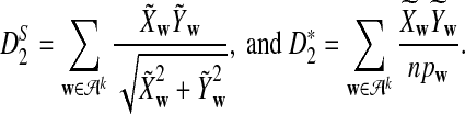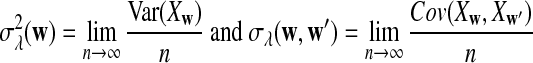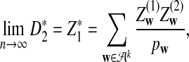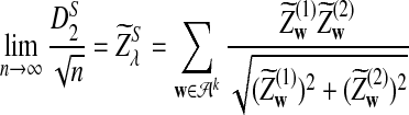The statistic is based on centered counts, divided by the square root of their means, whereas is a self-standardized statistic. More specifically, let X_w and Y_w be the numbers of occurrences of word w in the first and the second sequences, respectively. The D₂ statistic is defined as

To define and as in [9], we first introduce the centralized count variables by

where p_w is the probability of word w under the null model. Then we put

Here we set .

The power of those statistics under two alternative models were explored via simulation approaches. The first alternative model is that the two sequences contain random instances of a common motif, whereas the second alternative model is a pattern transfer model, where randomly chosen DNA segments in the first sequence are used to replace corresponding segments in the second sequence.

It has been shown that, under the first alternative model, the power of both and is an increasing function of the sequence length for any tuple size k ≥ 2, while the power of D₂ does not necessarily increase with sequence length and sometimes can even be smaller than the pre-specified type I error. In almost all the simulations considered, the power of is higher than that of . Under the second alternative model, the power of both and quickly reaches their plateau and does not seem to change with sequence length. The power of D₂ can decrease with sequence length in some examples.

Simulation studies can only explore very limited ranges of parameter values to compare the power of detecting the relationship between two sequences or genomes. To compare the performance of the different statistics under a broad range of evolutionary scenarios, theoretical studies of the power of these statistics are needed. In addition, it should be very useful to have an easy to use program for calculating the power of sequence comparisons using the various statistics without resorting to time consuming simulations. In this article, we achieve the following objectives: (1) to study the limiting distributions of D₂, , and under the two alternative models; (2) to compare the theoretical approximate mean, variance, and power of D₂, , and with the corresponding simulated values (we show that the approximations are reliable for D₂ and . However, for the approximations of to be reasonable, very long sequences are usually needed); (3) and to develop a program to calculate the power of detecting the relationship between two sequences using D₂, , as well as . As our calculations are based on approximations, we note that the power in this article is approximate. For easier exposition we omit the word “approximate”; any power is understood to be approximate.

The organization of the article is as follows. In Section 2, we give details of the alternative model I, and show that the distributions of 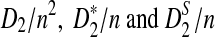converge to normal distributions as the sequence length tends to infinity. Formulas for the approximate mean and variance of are presented, and they are put to use to calculate the power of D₂, and . In Section 3, we give details of alternative model II and develop a new hidden Markov model (HMM) for generating pairs of sequences related through alternative model II. The approximate distributions of D₂, , and under alternative model II are then derived. These approximate distributions are not normal and are complicated. We show that the power of D₂, , and converges rapidly and does not change much as sequence length n increases, a phenomenon observed in the simulation studies of Reinert et al. (2009). Under the second model, we do not have an efficient method for calculating the mean and variance of , but we are able to present methods for calculating the approximate mean of D₂ and . In Section 4, we first describe a web-based and a R program package for calculating the power of D₂, and to detect the relationships between two sequences under alternative model I. We then evaluate the program by comparing the theoretical mean, variance, and power derived in this study with the corresponding simulated quantities presented in Reinert et al. (2009) and show that the approximate mean and variance are generally close to their corresponding true values when the sequence length is very large. We find that convergence for is considerably slower than for and for D₂. This also affects the power of the statistic—the power approximation for is poor in the parameter regimes we considered. Hence, we concentrate on D₂ and for the remainder of the article. Moreover, D₂ has zero power under some models, and hence cannot be used to infer the relationship between sequences under such models. For D₂ and , the program developed in this study can be readily used to study the power of comparing sequences using k-tuples. We then extend our study to 323 transcription factor (TF) binding motifs and show the superiority of compared to D₂ for sequence comparison for general motif patterns although there are a few exceptions where D₂ is more powerful than . For alternative model II, we study how the means of D₂ and change with the word length k in order to explain the observation that the power of using k = 10 is much higher than the power using k = 5 in the simulation studies reported in Reinert et al. (2009). The article concludes with some discussion and potential extensions to more general background sequence models.

The results regarding the approximate distributions of D₂, , and and the power of detecting the relationships between the sequences using these statistics can be easily extended to sequence pairs with different background letter frequencies, sequence lengths, and motif densities. However, the notation and presentation will be more complicated. For notational simplicity and clarity of presentation, we present the results for two sequences having the same background probability distribution, sequence length, and motif density. The results for the general situations are given in the Appendix. As the proofs are very similar to the ones presented in the article, they are omitted.

2. Alternative Model I

2.1. The model and the count statistics

The alternative model I renders the two sequences dependent through a common motif which is randomly distributed across the two sequences. As in Reinert et al. (2009), we model the background sequence as independent identically distributed (IID) random variables taking different letters from finite alphabet with probability . For notational convenience, we also denote . For nucleotide sequences, and for amino acid sequences, the is the set of 20 amino acids. In general, we assume that contains L letters and write . For the motif instances, we use the model in Zhai et al. (2010), which is more general than the model used in Reinert et al. (2009), where fixed motifs were used. In this article and in Zhai et al. (2010), a position weight matrix (PWM) is used to describe the distribution of the nucleotides at the different positions of a motif (Stormo, 2000). For a given motif of length M, and at the m-th position of the motif, the probability that the base takes value a from is . The motif instances are randomly distributed across the sequence with density 1 − λ (0 < λ < 1). That is, at each position in the sequence which is not already covered by an instance of a motif, with probability λ, a base with the background distribution is generated, and with probability 1 −λ, an instance of the motif of length M is generated based on the PWM for the motif. Once an instance of a motif is generated, we move to the end of the instance of the motif to repeat this process.

For the model in more detail, see Zhai et al. (2010). The sequences with random motif instances were modeled by an HMM (Rabiner, 1989). The underlying Markov chain (MC) of each sequence is denoted as (i is the position index of the sequence with length n + k − 1) which take values in . The 0 indicates that the state of the sequence is the background sequence while m (1 ≤ m ≤ M) indicates the state at the m-th position of the motif. Under each state, the emission probability of each letter from is denoted as . The transition matrix for the underlying MC is given by , where , and all the other t's are 0. The MC has as stationary distribution (Zhai et al., 2010). Therefore, in stationarity, the expected fraction of the sequence that is covered by the motif instances is M(1 − λ)/(λ + M(1 − λ)). Unless λ is close to 1, the expected fraction of the sequence covered by inserted motif instances can be unrealistically large (Table S1; for Supplementary Material, see www.liebertonline.com/cmb). Hence we only study values of λ which are no smaller than 0.9.

Now we consider two sequences of length n + k − 1 generated by the above HMM, and . We let the sequence length be n + k − 1 for notational simplicity in the remainder of the paper. Given a k-tuple 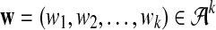, let X_w and Y_w be the numbers of occurrences of w within A and B, respectively; within each sequence, the occurrences could overlap. Assume that the Markov process starts in the stationary distribution. Based on Proposition 2.2 in Zhai et al. (2010), the means of X_w(n) and Y_w(n) can be calculated as

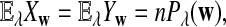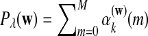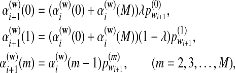
where is the probabiltiy of the word w under the alternative model I. The , are calculated recursively using the standard forward procedure for calculating the probability of an observation sequence based on HMM (Zhai et al., 2010; Rabiner, 1989) for :

and

In particular, .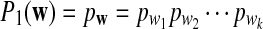

2.2. The expectations of D₂, and under alternative model I

It is easy to see that 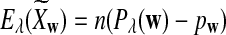, where P_λ(w) is the probability of word w under the alternative model I. However, for the mean of 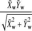, it is in general only known that it is non-negative, and when and are IID, the mean is zero if and only if the distribution of is symmetric (Novak, 2007). Note that the two sequences A and B are independent under the alternative model I. Then, we have the following theorem.

Theorem 2.1

Assume alternative model I for the two sequences A and B, and let be as calculated in Subsection 2.1. Then for the expectations of D₂, and , we have

Further,

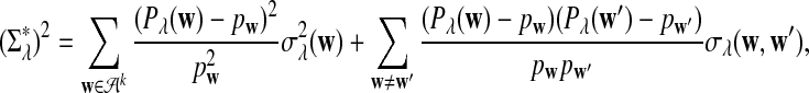
where 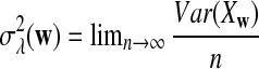; see also (1) below.

The first two equations can be easily proven by the independence of the two sequences. The last two limit expressions can be proven by Taylor expansion (the delta method); see the proof of Theorem 2.4 for details.

2.3. The approximate distributions of D₂, , and under alternative model I

The variances of D₂ and its variants are complicated. Under the null model of IID sequences, upper and lower bounds for the variance of D₂ were first explored in Lippert et al. (2002). In Kantorovitz et al. (2007b), an explicit formula for the variance of D₂ is given in the IID case. To study the power of D₂, , and in detecting the relationship between two sequences, we explore the approximate distributions of these statistics as the sequence length goes to infinity. Note that the distributions of D₂ and under the null model when 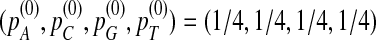have been carefully studied in Reinert et al. (2009). Therefore, in the rest of the article, we assume that .

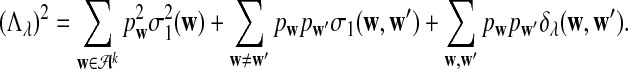
For 0 < λ < 1, the values of

(1)

can be calculated using the method in Zhai et al. (2010), Proposition 2.3; for λ = 1, the corresponding values can be found, for example, in Reinert et al. (2009), Corollary 6.1. We denote the asymptotic variance of 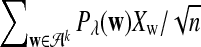in one sequence by

(2)

The following theorem gives the approximate distributions of D₂ under the null and the alternative model I.

Theorem 2.2

Assume that in the background model not all letters are equally likely.

a. [Lippert et al. (2002), Theorem 4.2.] Suppose λ = 1 (the null model that the sequences are IID). Then

where Z₁ has normal distribution . Here the asymptotic is valid when the sequence length tends to infinity with alphabet size, motif length, and word length kept fixed.

b. Suppose 0 < λ < 1 (the alternative model I). Then

where Z_λ has normal distribution . Here the asymptotic is valid when the sequence length tends to infinity with alphabet size, motif length, and word length kept fixed.

On the other hand, under the null model that no motif instances are inserted, is approximately the sum of products of dependent mean 0 normal random variables (and thus not normal). However, it is approximately normally distributed when the sequence length is large under the alternative model I, as long as is not constant in w, as the following theorem shows. We put

(3)

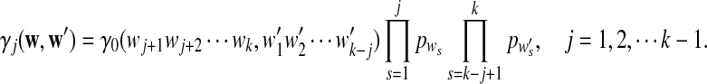
with and σ_λ(w, w′) given in (1).

Theorem 2.3

• a. Suppose λ = 1 (the null model that the sequences are IID). Then, in distribution,

  

  where and 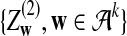are independent and have the same mean 0 normal distribution (with non-trivial covariance matrix).

• b. Suppose 0 < λ < 1 (the alternative model I), and that is not constant in w. Then, in distribution,

  

  where has normal distribution .

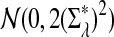We let

(4)

where sign(x) = 1 if x > 0, sign(x) = −1 if x < 0, and sign(0) = 0; again and σ_λ(w, w′) are given in (1). The following theorem gives the approximate distribution of under the null and the alternative models.

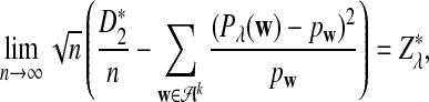
Theorem 2.4

• a. Suppose λ = 1 (the null model that the sequences are IID). Then, in distribution,

(5)

• where and are independent and have the same mean 0 normal distribution.

• b. Suppose 0 < λ < 1 (the alternative model I), and assume that P_λ(w) − p(w) have different sign in w. Then, in distribution,

• where has normal distribution .

• c. Suppose 0 < λ < 1 (the alternative model I), and assume that P_λ(w) − p_w have different sign in w. Then, in distribution,

• where has normal distribution .

Remark 2.1

Since each term on the right hand side of (5) has a normal distribution under the null model by Reinert et al. (2009), and the terms are jointly normal, the limit of is mean zero normally distributed. The variance can be estimated from the empirical distribution, as illustrated in Reinert et al. (2009).

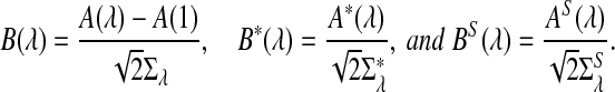
Replacing by can be significant when we study the power of detecting the relationships between two sequences using , as we shall see in Section 4.2.

The proofs of these theorems are presented in the Appendix.

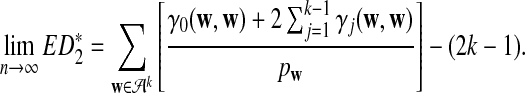
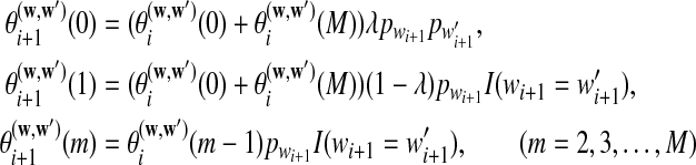
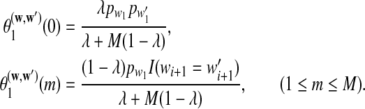
2.4. The power of detecting the relationship between two sequences under alternative model I using D₂, , and

Knowing the asymptotic distributions of D₂, , and under the null and the alternative models, we are able to approximate the power of detecting the relationships between two sequences using any of the three statistics. For notational simplicity, let

denote the (asymptotic) means of D₂, , and under alternative model I. Let Φ(·) be the cumulative distribution for the standard normal distribution. From Theorems 2.2, 2.3, and 2.4, we can show the following theorem to hold.

Theorem 2.5

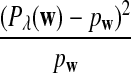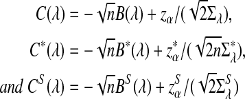
Assume that and P_λ(w) − p_w are not constant in w. Then, for any given type I error α, the power of detecting the relationship between two sequences against the null model that λ = 1 using D₂, and can be approximated by 1 − Φ(C(λ)), 1 − Φ(C*(λ)), and 1 − Φ(C^S(λ)), respectively, where

and

Here, z_α, , and are the upper α quantile of Z₁, from Theorems 2.2, 2.3, and 2.4, respectively.

Note that we can again replace A^S(λ) by 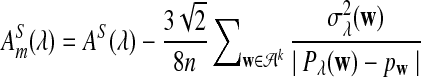when we calculate the power of for relative small values of sequence length n. Here the subscript m stands for modified.

Theorem 2.5 indicates that when sequence length n is large, the dominant terms in C(λ), C^*(λ), and C^S(λ) are the first term and the second term becomes negligible when n is large. Therefore, the higher the values of the B's, the more powerful the corresponding statistic is when n is sufficiently large. In Section 4, we present some examples for values of the B's and the C's.

The tests under alternative model I make extensive use of the fact that the means of our statistics are different under the alternative model versus the null model. Under alternative model II, this will turn out not to be the case.

3. Alternative Model II

In this section, we consider the second alternative model which is inspired by horizontal gene transfer. We randomly choose a certain number of segments in the first sequence and then replace the corresponding segments (position-wise) in the second sequence by the letters in the first sequence.

3.1. A second HMM model for the sequence pair A and B

Alternative model II is again a HMM model for the sequence pair 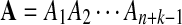and . First, two IID sequences A and B′ are generated. From these two sequences we construct B as follows. We assume that at each position which is not already covered by a chosen segment, with probability λ, the original bases of the two sequences at the position are kept. With probability 1 − λ, a segment of length M from the first sequence is chosen, and the same segment in the second sequence is replaced by it. Then we move to the end of the segment to start this process again. Consider an underlying Markov chain defined as follows. Each Q_i takes values in , where Q_i = 0 indicates that, at position i, A_i and B_i are the originally generated bases, whereas 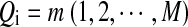indicates that position i is at the m-th position of a segment which was copied from the first sequence to the second sequence. The transition matrix of is given by , where , and all the other t's are 0. It is easy to see that the stationary distribution of this Markov chain is 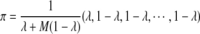(see Proposition 2.1 in Zhai et al. [2010]).

Let C_i = (A_i, B_i)^t. With p_a denoting the probability of letter a in the IID model, the emission probabilities are given by

Then form a HMM.

3.2. The asymptotic distributions and power of D₂, , and for detecting relationships between sequences under alternative model II

Under alternative model II, the marginal distributions of the individual sequences are IID sequences and hence the means of X_w and Y_w are unchanged compared to the IID model. However, the two sequences depend on each other because they share some common segments. The following theorem shows an efficient way to calculate the covariance of the number of occurrences of word w in sequence A and the number of occurrences of word w′ in sequence B. These covariances are used to derive the limiting distributions of D₂, , and when the sequence length tends to infinity.

Theorem 3.1

Let X_w and Y_w be the number of occurrences of word w in sequence A and B, respectively. Assume that the MC starts in the stationary distribution. For any pair of words (w, w′), we have under alternative model II,

• a. The expectation of X_wY_w′ is

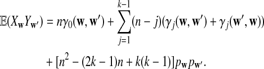• b. The covariance of X_w and Y_w′ changes linearly with sequence length n, and

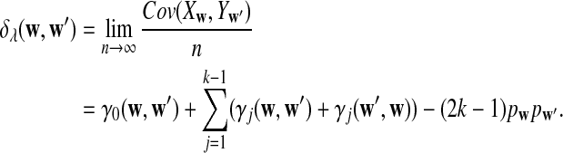(6)

• c. The difference changes linearly with respect to sequence length n, and

(7)

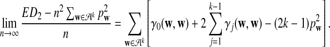
• d. The expectation of converges as the sequence length n tends to infinity, and

(8)

In all the above equations, can be calculated as , and can be calculated recursively using the following equations for

with initial values

Moreover can be calculated as

Similarly to the proofs of Theorems 2.2, 2.3, 2.4, we can prove the following theorem regarding the limiting distributions of D₂, , and . Let and , which can be calculated as in Zhai et al. (2010), and recall δ_λ(w, w′) from (6).

Theorem 3.2

Suppose 0 < λ ≤ 1 and the alternative model II.

• a. Then, in distribution,

• where has normal distribution 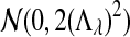, and

• b. In distribution,

• where and have the same marginal normal distribution N(0, (σ₁(w, w′))_w,w′) and the covariance between and is δ_λ(w, w′).

• c. In distribution,

• where and are the same as in part (b).

Based on the above theorem, we can obtain the approximate power of D₂, , and for detecting the relationships between two sequences under the alternative model II.

Theorem 3.3

Suppose 0 < λ < 1 and the alternative model II. For a given type I error α, let , and be the upper α quantile for 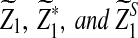, respectively. Then the corresponding power of 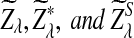under the alternative model II when λ < 1 is asymptotically 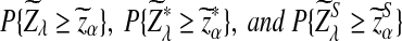, respectively.

Since is normally distributed with mean 0, the threshold value if α < 0.5. From this theorem, it is clear that the power of the three statistics for detecting the relationships between the two sequences does not increase with sequence length n when n is sufficiently large, which is consistent with the simulation results in Reinert et al. (2009). The theoretical results presented here explain that none of the three statistic is what would be most desirable for detecting the relationships between sequences under the alternative model II. One unsolved problem is what statistics we should use under alternative model II.

4. Results

In this section, we describe an online implementation and a stand-alone R program for calculating the power of detecting the relationships between two sequences under the alternative model I using any of the statistics studied in this article. Then we compare the mean, variance, and power of the statistics D₂, and derived using our formula with the simulated quantities for the situations in Reinert et al. (2009). As an illustration of the difficulties involved, we present the results for the relatively simple two letter sequences under alternative model I in the supplementary material. In particular, this simple case shows that in some cases D₂ will have zero power for detecting the relationship between two sequences when they share a common motif. In some scenarios, however, we see that D₂ can be more powerful than and . It also shows that the convergence of the mean and variance of to their theoretical limit is very slow, which affects the approximate power calculation; in the parameter region which we considered, the theoretical approximate power of differs so considerably from the power under simulation that we do not recommend using for moderate sequence lengths. Finally, the power of detecting the relationships between two sequences when any of the 323 motifs with motif length at most 10 in JASPAR (Sandelin et al., 2004) (October 12, 2009 version) are present in the two sequences are given. For alternative model II, we give an explanation why the power of using k = 10 is much higher than using k = 2, 3, 4, 5 for the parameters in simulation studies (Reinert et al., 2009).

4.1. A program for calculating the power of detecting the relationships between two sequences under alternative model I

To facilitate the use of or for sequence or genome comparison and for evaluation of statistical power for detecting the relationship between the sequences, a web-based online program (http://meta.cmb.usc.edu/d2) and a stand-alone R program were developed to calculate the power of sequence comparison using these statistics. We describe the program for the above model. However, the program can be easily extended to the general scenario of different background letter frequencies, sequence lengths, and motif densities as in the supplementary materials. The inputs of the program are:

1. The background nucleotide or amino acid frequencies of the two sequences A and B under study;

2. the nucleotide or amino acid frequencies at each position of the motif (PWM);

3. the lengths n of the sequences A and B;

4. the motif density, 1 − λ, for the sequences A and B;

5. the type I error, α.

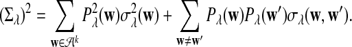
For each set of parameters, the program first calculates the mean for any word w and the covariance σ_λ(w, w′) = Cov(X_w, X_w′) for two words w and w′, related to sequence A. The corresponding quantities related to sequence B are also calculated. Secondly, the program calculates the approximate variance, of D₂, , and using formulas derived in Theorems 2.2, 2.3, and 2.4, respectively. Thirdly, for the given type I error α, the threshold values z_α, , and for the corresponding statistics D₂, or in Theorem 2.5 are calculated. Since the cumulative distribution functions of and are not readily available, a simulation based method is used to obtain the threshold values. A large number of independent sequence pairs are simulated according to the specified letter frequencies and the sequence lengths, and the empirical distributions of and are estimated. The threshold values are estimated by the upper α% quantile of the simulated values of each statistic. Finally, the values of C(λ), C^*(λ), and C^S(λ), and thus the power using the corresponding statistics in Theorem 2.5 is calculated.

We use the program to study the power of detecting the relationship between related sequences under alternative model I using the different statistics. In Subsection 4.2, we present the results for the parameter sets used in Reinert et al. (2009) and compare the results derived using our program with the simulated quantities in previous studies. In Subsection 4.3, we present the power of the various statistics for comparing the relationships between sequences when any of the motifs with motif length at most 10 in JASPAR (Sandelin et al., 2004) are present in both sequences.

4.2. Comparison of theoretical mean, standard deviation, and power of D₂, , and with their corresponding simulated values from Reinert et al. (2009)

In this subsection, we present some numerical results on the mean, standard deviation, and power of detecting the relationships between two sequences for the three statistics D₂, , and under the alternative model I using the same set of parameters as in Reinert et al. (2009). The objective is to see how close the corresponding quantities calculated using our formulas approximate the true values. We let the background letter frequencies for the two sequences be p_A = p_T =, p_C = p_G = . The inserted motif is “AGCCA” and the motif density 1 − λ = 0.01. The size of the k-tuple is k = 5. We used 10,000 simulations to find the threshold values z_0.05, , and . The type I error α was set at 0.05 and 0.01.

For scaled D₂, , and defined respectively by

from Theorems 2.2, 2.3, and 2.4, it can be seen that the (approximate) means are , respectively. Similarly, the approximate variance of ND₂, and are , respectively.

Table 1 shows the simulated mean and standard deviation of , and , respectively, and their corresponding limits. Surprisingly, the approximate mean and standard deviation of ND₂ are within 15% of their limit even when the sequence length is just 1Kbp. For , the simulated mean is roughly the same as the theoretical limit and the simulated standard deviation is within 21% of its theoretical limit when the sequence length is at least 1Kbp. However, the simulated mean of is much smaller than its limit. The corrected mean for is very different from the simulated mean, too, probably because the difference between P_λ(w) − p_w for most 5-tuples are very small; both approximations do not work well in this parameter regime. Therefore, while we expect that the power formulas we derived should approximate the true power of D₂ and well even for sequences of over 1Kbp long the power formula for can significantly over-estimate the true power.

Table 1.

Comparison of Simulated Mean and Variance of ND₂, , and for Different Sequence Length n with the Corresponding Theoretical Limits (the last row), with (p_A, p_C, p_G, p_T) = (1/6, 1/3, 1/3, 1/6), λ = 0.99, Motif = “AGCCA”, and Word Length k = 5

	D2
n * 10−4		σ(ND2) * 103
0.1	0.92	4.09	1.34	2.41	4.35	−1032	6.80
0.12	0.92	4.12	1.33	2.34	4.03	−859	7.01
0.14	0.94	4.08	1.34	2.34	3.73	−735	7.15
0.16	0.97	4.03	1.34	2.27	3.60	−642	6.99
0.18	0.98	4.01	1.35	2.23	3.51	−570	7.07
0.2	0.98	3.95	1.35	2.24	3.38	−512	7.05
0.3	0.99	3.90	1.33	2.14	3.35	−339	7.32
0.4	1.01	3.86	1.34	2.11	3.48	−252	7.39
0.5	1.02	3.85	1.34	2.09	3.57	−200	7.47
0.6	1.03	3.84	1.34	2.08	3.66	−165	7.61
1	1.03	3.82	1.34	2.05	3.98	−96	7.90
2	1.04	3.80	1.34	2.03	4.48	−44	8.38
20	1.04	3.71	1.34	2.00	6.46	2.8	9.32
1000	1.05	3.76	1.34	1.95	7.90	7.89	7.83
Theory	1.05	3.76	1.34	1.99	7.99	7.99	7.72

As before, σ denotes standard deviation.

Table 2 shows the theoretical approximate power of D₂, , and calculated using our formulas and the simulated power with the same setting as in Table 1. The results show that the approximations are very close for D₂ and . However, the theoretical approximate power based on the first approximation significantly over-estimates, while the approximate power based on the second approximation significantly under-estimates the simulated power for , in the parameter regime we consider.

Table 2.

Comparison of the Theoretical and the Simulated Power Under Alternative Model I for Different Values of Sequence Length, with (p_A, p_C, p_G, p_T) = (1/6, 1/3, 1/3, 1/6), λ = 0.99, Motif = “AGCCA”, and Word Length k = 5

	D2
n * 10−4	Theory	Simulated	Theory	Simulated	Theory1	Theory2	Simulated
Type I errorα = 5%
0.1	21	20	85	81	87	0	33
0.12	25	23	91	88	94	0	39
0.14	29	26	95	93	98	0	45
0.16	32	29	97	97	99	0	52
0.18	32	29	98	98	100	0	57
0.2	38	35	99	99	100	0	62
0.3	49	45	100	100	100	0	81
0.4	59	55	100	100	100	0	93
0.5	66	63	100	100	100	0	97
0.6	73	71	100	100	100	0	99
1	90	89	100	100	100	0	100
2	99	99	100	100	100	0	100
20	100	100	100	100	100	100	100
1000	100	100	100	100	100	100	100
Type I errorα = 1%
0.1	4	5	71	66	72	0	16
0.12	7	8	82	77	83	0	18
0.14	8	9	88	84	91	0	21
0.16	11	11	93	92	96	0	29
0.18	11	11	96	96	98	0	33
0.2	14	14	97	97	99	0	36
0.3	22	20	100	100	100	0	60
0.4	31	28	100	100	100	0	81
0.5	38	36	100	100	100	0	90
0.6	45	43	100	100	100	0	96
1	71	70	100	100	100	0	100
2	96	96	100	100	100	0	100
20	100	100	100	100	100	100	100
1000	100	100	100	100	100	100	100

As before, σ indicates standard deviation.

As the approximate power for is not accurate in the parameter regimes we have considered, in the following, we only show the results related to D₂ and using the theoretical approximate power. Figure 1 shows the values of C(λ) and C^*(λ) (upper panel) and the power of D₂ and for detecting the relationships between pairs of sequences (lower panel) as a function of sequence length and the word length k when λ = 0.99. It should be noted that the power is a decreasing function of the values of C's and the smaller the values of C, the higher the power of the corresponding statistic is. From the left panel related to D₂, it can be seen that, when k = 2 or 3, the value of C actually increases and that the power 1 − Φ(C(λ)) decreases with the sequence length. For given sequence length and word size k, the power of is generally higher than the power of D₂. All these conclusions are consistent with the simulation studies in Reinert et al. (2009). Comparing the two figures in the lower panel of Figure 1 here with Figures 1 and 2 in Reinert et al. (2009), respectively, we can see that the the theoretical power is slightly higher than the simulated power, but the difference is generally small, less than 10% in all the situations considered.

FIG. 1.

The values of C(λ) and C^*(λ) (upper panels) and the power of D2 and (lower panels) for detecting the relationships between sequence pairs related through alternative model I for different values of word size k = 2, 3, 4, 5 and sequence length n. The parameters were set at p_A = p_T = 1/6, p_C = p_G = 1/3, λ = 0.99, and type I error α = 0.05.

FIG. 2.

The values of B(λ) and B^*(λ) for λ = 0.93, 0.99 and k = 2, 3, 4, 5. Dashed lines refer to B and solid lines to B^*; triangles refer to λ = 0.93 and circles to λ = 0.99. B(0.99), dash line with circle points; B(0.99), dash line with triangle points; B^*(0.99), solid line with circle points; B^*(0.99), solid line with triangle points.

Simulation studies can only explore the influence of a relatively small range of parameter sets on the power of the different tests. With the theoretical results presented in this paper, we are able to explore a much larger parameter space. Theorem 2.5 shows that the power of D₂ and is mainly determined by B(λ) and B^*(λ), respectively. The higher the values of B's, the more powerful the test is. Therefore, we also plot the values of B(λ) and B^*(λ) for k = 2, 3, 4, 5 and λ = 0.93 or 0.99 (Fig. 2). Again it is shown that B^*(λ) is generally larger than B(λ) indicating that is generally more powerful than D₂. We note that both B and B^* decrease when λ increases. The smaller λ is, the larger is the probability of inserting a motif, and the eaiser it is to detect a difference from the null model.

4.3. The power of D₂ and for comparing two sequences when motifs in JASPAR are present

Since the approximate distribution of in Theorem 2.4 requires very long sequences and the resulting formula for calculating the power of significantly over-estimates the true power, we will not consider in the following. We next investigate whether the relative performance of D₂ and for comparing the relationships between two sequences holds for a large class of motifs. To achieve this objective, we downloaded the transcription factor (TF) binding sites in the database JASPAR CORE (Sandelin et al., 2004) as motifs and studied the power of detecting the relationship between two sequences if such motifs are present in the sequences. The same letter frequencies for the background as in Reinert et al. (2009) are used. The theoretical formulas obtained in this paper make such large scale comparisons possible. Due to the long computational time required when the motif length is large, we only consider motifs with length at most 10.

A total of 323 transcription factor binding profiles with length at most 10 from JASPAR CORE (Sandelin et al., 2004) (October 12, 2009 version) are currently available. These motifs represent the most abundant publicly available knowledge regarding nucleotide sequence motifs. The corresponding PWMs are used to insert motifs as in alternative model I. Based on these assumptions, we can calculate the values of B(λ), B^*(λ), C(λ), C^*(λ), and the corresponding power for different values of word length k and motif density 1 − λ. The resulting figures and the corresponding letter frequencies in each position for all the motifs are presented in the supplementary material. From this large-scale study, we can conclude that is more powerful than D₂ in more than 90% of the motifs. An example motif profile “MA0003” for which D₂ is more powerful than is given in Figure 3. Note that in this motif, the overall frequencies of (A, C, G, T) in the motif are (0.11, 0.40, 0.40 0.09).

FIG. 3.

The sequence LOGO of motif “MA0003”.

We then calculate the mean overall letter frequencies of (A, C, G, T) in those motifs for which D₂ is more powerful than for at least three of the k = 2, 3, 4, 5 (λ = 0.93) and the corresponding frequencies are (0.08, 0.22, 0.57, 0.13). On the other hand, the mean overall letter frequencies of (A, C, G, T) in the other motifs are (0.30, 0.22, 0.25, 0.23). Under the background sequence model with (A, C, G, T) frequencies equal to (1/6, 1/3, 1/3, 1/6), in general, the GC content of the motifs for which D₂ is more powerful than is higher than that of the other motifs under the background model considered in this article. If the background sequence model is changed, the PWM of motifs for which D₂ outperforms should also change. As a general rule, D₂ outperforms if the letter frequencies in a motif are close to the background letter frequencies.

Since we found that, in most situations, the power of D₂ can be even smaller than the type I error, whereas the power of always approaches 1 for sequence length tending to infinity, we do not suggest using D₂ in general situations even if it can potentially perform well in some special cases.

4.4. The power of D₂, , and for detecting the relationships between two sequences under alternative model II

Previous simulation studies have shown that, under alternative model II, the power of D₂ is less than 0.4 and decreases with sequence length n when the word size k is 2 to 6. Actually, we can show that when n is large, the power of D₂ is always less than 0.5 for any parameter set. Note that Theorem 3.3 shows that the power of D₂ is approximately . Since is positive and is approximately normally distributed, the power is less than 0.5 when the sequence length is large for any set of parameters. However, similar arguments will not work for and since the distributions of and are not normal when λ < 1. This shows that D₂ does not have enough power to detect the relationship between sequences under alternative model II. So we will not study D₂ further under alternative model II. Previous simulation studies also showed that is less powerful than . So we now concentrate on further understanding and .

Theorems 3.2 and 3.3 show that the power of detecting the relationships between two sequences related through the alternative model II using any of D₂, , and reaches its plateau quickly as the sequence length increases, and the limit is generally much smaller than 1. Theorems 3.2 and 3.3 justify the simulation results that the simulated power by any of the statistics tends to a limit which is typically less than 1 when sequence length goes to infinity (Reinert et al., 2009), which was quite intriguing at the time of the simulation studies. Let T be any one of statistics D₂, , and . It is theoretically shown here that the primary reason for the power of T to be stable with respect to sequence length n is that there exist constants a_n and b_n such that U_λ,n = a_n(T − b_n) approximates non-degenerate random variables U_λ under both the null model (λ = 1) and the alternative model λ < 1. Although U_λ is stochastically decreasing with respect to λ, the power of the test approaches a constant P(U_λ ≥ u_α), where P(U₁ ≥ u_α) = α. In order for the power of T to increase with respect to sequence length n and to finally reach 1, we need that (1) U_1,n approximates a non-degenerate random variable U₁ under the null model (λ = 1), and (2) U_λ,n tends to infinity as n tends to infinity.

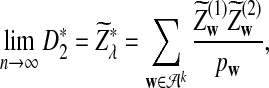
Another interesting observation from previous simulation studies is that the power of seems to increase with the length, k, of word pattern used (see Figure 8 in Reinert et al. (2009)). In order to explain this phenomenon, we study the mean as a function of word length k. We are aware that in general the power of a test depends on the distributions of the test statistics under the null and the alternative hypothesis, not just the mean and/or the variance. However, as an explanation to the intriguing observation, we try to see if increases with k when other parameters are fixed. Theorem 3.1 (d) shows that

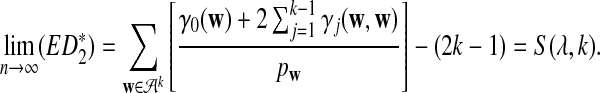Figure 4 shows the relationship between S(λ, k) and for k = 2, 4, 6, 8, 10. It can be seen that S(λ, k) increases with k for any , as does the discrepancy between S(λ, k) and S(1, k) for λ < 1. As our statistic is based on comparing the means of the counts under the two models, this partially explains that the power of increases with word length k.

FIG. 4.

The values of as a function of motif density λ and word length k, λ = 0.9 to 1.0 by step 0.01, and

5. Discussion

Alignment-free sequence comparison has become increasingly important as new sequencing technologies can generate enormous amount of sequence data in a relative short time and at low cost. However, the statistics used for alignment-free sequence comparison are usually ad-hoc, and it is not clear whether such ad-hoc statistics can actually find the relationships between sequences. It is also important to know under which evolutionary models the statistics are meaningful. One of the widely discussed and studied statistics for alignment free sequence comparison is the D₂ statistic. Previously simulation studies have shown the limitations of D₂ in detecting the relationships between sequences under a common motif model (alternative model I) and a pattern transfer model (alternative model II). It was shown that the power of D₂ can even be smaller than the pre-specified type I error under some situations. Two new statistics, and , were developed to overcome the inherent problems of D₂ and simulation studies showed their superior performance compared to D₂ (Reinert et al., 2009).

However, the approximate distributions of these statistics were not known at the time of the study (Reinert et al., 2009), and thus, it was not possible to give a theoretical formula to calculate the power of the different tests. Having the limiting distribution of the test statistics can help us design algorithms to calculate the power. With the power calculator, we are able to explore a large range of the parameter space and study how the parameters individually and collectively contribute to the power of the tests. The theoretical studies also give insights into when and how the test statistics can be applied to compare sequences. In this paper, we carried out a systematic theoretical study of the power of D₂, and for detecting the relationships between sequences under alternative models I and II. Under alternative model I, we provided an easy to use program to calculate the power of the test statistics D₂ and for different combinations of parameters. Using the program, we then obtained the theoretical power and compared with the simulated power using the same parameters as in Reinert et al. (2009) and showed that they are generally close, thus validating the usefulness of our program. However, the convergence of to our theoretical limit is very slow and the approximation is only reasonable for very long sequences. We then carried out a large-scale comparison of D₂ and statistics for sequence comparison under alternative model I when the motif is any one of the 323 motifs with length at most 10 in JASPAR CORE. Our program made such a large-scale comparison possible. We verified the relative performance of D₂ and observed in previous studies, i.e. is generally more powerful than D₂. Under alternative model II, we theoretically showed that the power of the three statistics tends to a constant, usually less than 1. We also gave some reasons why the power of increases with the word size k.

This study has several limitations regarding the models of the background sequences and the foreground motif models. The IID model was used to model the background sequence. It is known that the genomes of organisms are hierarchically organized (Mantegna et al., 1994) and simple IID models cannot fully describe the background sequences; instead high-order Markovian models could be more appropriate. Similarly, the positions of the motifs are assumed independent and again this assumption can be violated in many motifs. To incorporate such complexity into our model, high-order HMMs can potentially be used; the calculations would then become much more involved. Although the extensions to higher order HMM are conceptually simple, heavy computational issues need to be solved.

We made several simple assumptions regarding the distribution of the motifs along the sequences as in Reinert et al. (2009). First it was assumed that the motifs are uniformly distributed along the sequences. Motifs can cluster together in some regions and may be sparse in other regions of the sequences. If such inhomogeneity is known to be present, an inhomogeneous HMM can be used to model the distribution of motifs by assuming large motif density λ in motif-clustered regions and low motif density λ in sparse motif regions. If such motif-clustered and motif-sparse regions are unknown, but suspected, we can assume that λ is a random variable following certain distributions. Second, we considered the presence of just one motif along the sequences. In many situations, several motif patterns work together to form modules. How to model such sequences is a problem for future studies. Third, we emphasize that the three statistics we consider here are most likely not optimal and other more powerful statistics may possibly be constructed. Fourth, applying these statistics to practical examples is another topic for future research.

In this article, we theoretically showed that, under alternative model II, the power of D₂, , and converges to a value that is generally much less than 1 when the sequence length tends to infinity. Therefore, they are not appropriate to test for relationships between sequences under this model. The obvious important question is which statistics based on word counts should be used for testing against this model instead.

6. Appendix A: Proofs of the Theorems

In this Appendix, we prove the theorems in the main text.

A.1. Proofs of Theorems 2.2–2.5 under alternative model I

Proof of Theorem 2.2

From the definition of D₂, we have

Therefore,

(9)

It has been shown in Zhai et al. (2010), Proposition 2.4, for 0 < λ < 1, and in Reinert et al. (2009), Proposition 6.1, for λ = 1, that, in distribution,

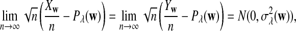(10)

where 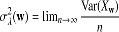. Therefore, the first term in equation (9) tends to 0 when n → ∞, with alphabet size fixed, and

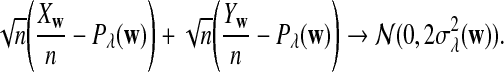Let which can be calculated as in Zhai et al. (2010) for 0 < λ < 1, and as in Reinert et al. (2009) for λ = 1. Since and are independent, the second term in (9) is asymptotically normal with mean 0 and variance 2(Σ_λ)². Theorem 2.2 is proved.

We note that the proof of Theorem 2.2 breaks down when all letters are equally likely, as then with p = p_w,

and thus the second term in (9) vanishes.

Proof of Theorem 2.3

The proof of Theorem 2.3 is similar to the proof of Theorem 2.2. The first part can be easily proved using the normal approximation Corollary 6.1 in Reinert et al. (2009) for the individual centered word counts, which also holds when all letters are equally likely. To prove the second part, note that

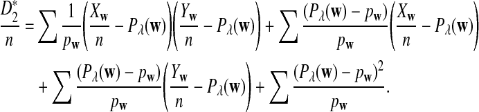It follows from the normal approximation for individual word counts that, in distribution,

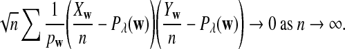Therefore, in distribution,

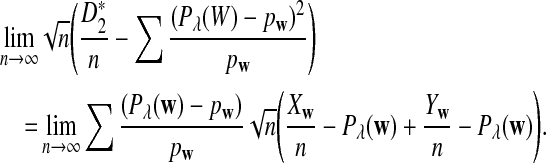For 0 < λ < 1, under the assumption that is not constant in w, this expression has a normal distribution with mean 0 and variance , where is given in (3). Theorem 2.3 is proved.

Proof of Theorem 2.4

The first part of Theorem 2.4 has been proved in Theorem 2.1 in Reinert et al. (2009). We only present the outline for the proof of the second part. Using Taylor expansion, it is straightforward to show that for any a ≠ 0 and (x, y) in the neighborhood of (0,0),

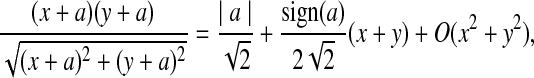where O(x² + y²) indicates a term such that there exists a constant C with

For each word w, let , and . Then, with this Taylor expansion,

(11)

Taking expectations in (11) we obtain that

As 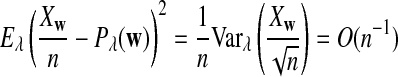, we obtain that the asymptotic mean of equals .

Moreover, summing Equation (11) over all the word patterns , we have

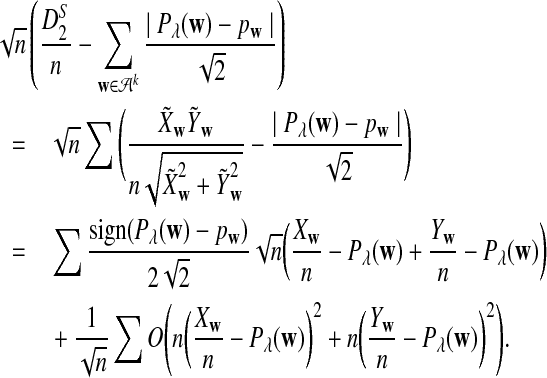Similar as in the proof of Theorem 2.2, under the assumption that P_λ(w) − p(w) is not constant in w, we see that 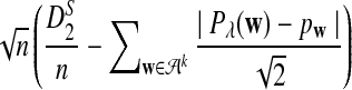is asymptotically normal with mean 0 and variance .

For the last assertion, we refine the Taylor expansion to

and using a = P_λ(w) − p_w, if P_λ(w) − p_w ≠ 0, , and , taking expectations completes the proof of Theorem 2.4.

Proof of Theorem 2.5

The proof of the three equations are roughly the same, and thus we only give the proof for the first equation.

Note that under the alternative model I, we expect that the k-tuple counts for the two sequences are more correlated than that for two random sequences. Therefore we use one-sided test. For fixed type I error α, based on Theorem 2.2 (a), we find z_α such that P{Z₁ ≥ z_α} = α. Under the null hypothesis that has approximate mean zero, whereas under the alternative λ < 1, the approximate mean of will not be zero. We reject the null hypothesis if Z₁ > z_α, which is approximately equivalent to 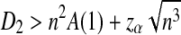. The power for D₂ is

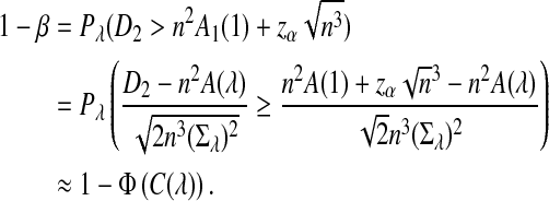The last approximation holds because of Theorem 2.2 (b).

A.2. Proofs of Theorems 3.1, 3.2, and 3.3

Proof of Theorem 3.1

We calculate for any two words w and w′ of length k. Let

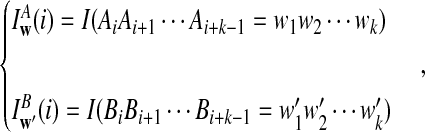then

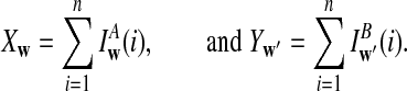Thus

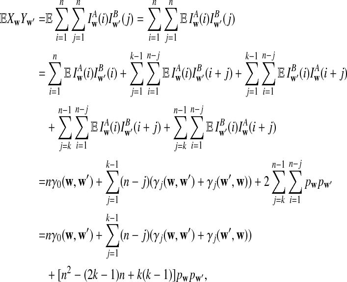where and . Part (a) of the theorem is proved.

Note that

Then part (b) can be easily deduced from part (a).

Part (c) and (d) can be proved by the definition of D₂ and , respectively, and by part (b) above by letting w = w′. The recursion follows as in Reinert et al. (2009).

Proof of Theorem 3.2

The proofs of parts (a), (b), and (c) of the theorem are similar to that of Theorems 2.2–2.4, respectively.

• (a) As in the proof of Theorem 2.2, we have

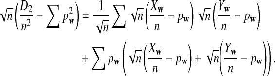(12)

• Under alternative model II, the marginal sequences are IID, and hence converges to a mean zero normal variable, call the asymptotic variance M₁; and converges to the same limit. As the two count vectors are asymptotically jointly normal, we obtain that, in distribution,

(13)

• where and .

Therefore, the first term in Equation 12 tends to 0 as n tends to infinity. The second term tends to a normal distribution with mean 0 and variance 2(Λ_λ)². Part (a) is proved. Parts (b) and (c) follow directly from the normal approximation (13).

Proof of Theorem 3.3

The proof of this theorem is similar to the proof of Theorem 2.5. For illustration only, we prove the claim for the power of . From Theorem 3.2 (b) with λ = 1, we can choose such that

We reject the null hypothesis that the two sequences are not related if . We use one sided test since the mean of is expected to be greater than 0 under the alternative model. From Theorem 3.2 (b), the test has an approximate type I error α under the null hypothesis λ = 1.

The power is the probability that the null model is rejected under the alternative model II λ < 1. Thus, the power is

Appendix B: Limit Distributions Of D₂, D₂^*, and D₂^S When The Two Sequences Have Different Letter Frequencies, Motif Densities, and Sequence Lengths

For simplicity of presentation, we have so far assumed that the two sequences have the same letter frequency, motif density, and sequence length. The theorems in the main text can be easily extended to the general situations. Let n_X be the length and 1 − λ_X be the motif density for sequence A. Let be the probability of pattern w under the null model and be the probability of word pattern w as calculated in subsection 2.1 for sequence A. Let and be similarly defined as in equations 2 and 3, respectively, by replacing λ with λ_X. Similar notation can be defined for sequence B; here we use the superscript or subscript Y. We define D₂ and similarly as above by replacing p_w by or appropriately. Let C_XY = n_X/n_Y. For simplicity of presentation, we also define C_YX = n_Y/n_Y = 1/C_XY. Under the general model, we redefine as

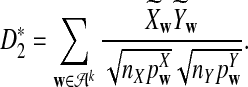In this general setting,

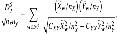(14)

From the law of large numbers we deduce that, in distribution and almost surely, 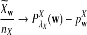, and a similar statement holds for . Hence, we abbreviate in connection with the asymptotic means, see Theorem 5.1

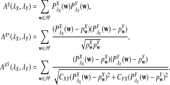where and in the following, the superscript “g” indicates the general model. In analogy to Theorems 2.1, 2.2, 2.3, 2.4, and 2.5, we have the following theorems. As the proofs are very similar to the ones presented in the article, they are omitted.

Theorem 5.1

Under alternative model I for the two sequences as described above, the expectations of D₂, and can be calculated as follows.

The limiting distributions of D₂, , and under the general model are given as follows.

Theorem 5.2

Assume that in the background model not all letters are equally likely.

• a. Suppose λ_X = λ_Y = 1 (the null model that the sequences are independent). Then

  

  where has normal distribution 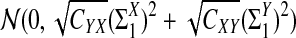. Here the asymptotics is valid when the sequence length tends to infinity with alphabet size, motif length, and word length kept fixed.

• b. Suppose 0 < λ_X, λ_Y < 1 (the alternative model I). Then

  

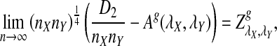
  where has normal distribution 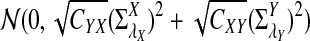. Here the asymptotics is valid when the sequence length tends to infinity with alphabet size, motif length, and word length kept fixed.

For , we have:

Theorem 5.3

• a. Suppose λ_X = λ_Y = 1 (the null model that the sequences are independent). Then, in distribution,

  

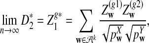
  where and are independent and have mean 0 normal distributions (with non-trivial covariance matrix).

• b. Suppose 0 < λ < 1 (the alternative model I), and that is not constant in w. Then, in distribution,

  

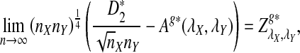
  where has normal distribution .

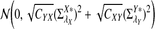In order to state the limit distribution for , we let

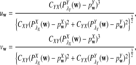and

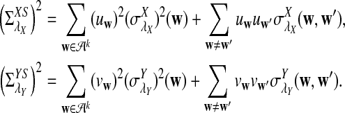The following theorem gives the approximate distribution of under the null and the alternative models for the general situation.

Theorem 5.4

• a. Suppose λ_X = λ_Y = 1 (the null model that the sequences are independent). Then, in distribution,

(15)

• where and are independent and have mean 0 normal distribution.

• b. Suppose 0 < λ_X, λ_Y < 1 (the alternative model I), and assume that both and are not constant in w. Then, in distribution,

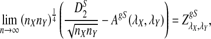• where has normal distribution .

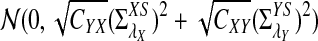The proof of Theorem 5.4 is sketched as follows. Similarly as for (14),

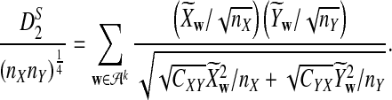For part (a), under the null hypothesis, we have that, in distribution,

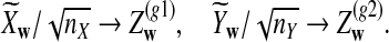For part (b), we can write

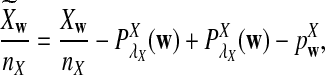Then we use Taylor expansion for the function g_w(x, y) given by

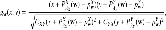at (x, y) = (0, 0), as well as (14).

From Theorems 5.2, 5.3, and 5.4, we are able to calculate the power of detecting the relationships between sequences A and B under the general model.

Theorem 5.5

Assume that are not constant in w. Then, for any given type I error α, the power of detecting the relationship between two sequences A and B against the null model that λ_X = λ_Y = 1 using D₂, and can be approximated by , respectively, where

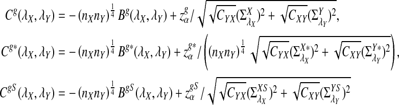and

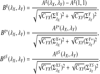Here, , and are the upper α quantile of from Theorems 5.2, 5.3, and 5.4, respectively.

The alternative model II can equally be extended to the situation of different letter frequencies in the two sequences; we omit the details here.

Acknowledgments

L.W. was supported by NIH grant no. P50 HG 002790 and by NIH grant no. R21AG032743. G.R. was supported in part by EPSRC grant no. GR/R52183/01, and by BBSRC and EPSRC through OCISB. F.S. was supported by NIH grants no. P50 HG 002790 and R21AG032743 and NSFC grants 60928007 and 60805010. M.S.W. was supported by NIH grant no. P50 HG 002790 and by NIH grant no. R21AG032743.

Disclosure Statement

No competing financial interests exist.

References

- Burden C.J. Kantorovitz M.R. Wilson S.R. Approximate word matches between two random sequences. Ann. Appl. Probab. 2006;18:1–21. [Google Scholar]
- Forêt S. Kantorovitz M.R. Burden C.J. Asymptotic behaviour and optimal word size for exact and approximate word matches between random sequences. BMC Bioinform. 2006;7:S21. doi: 10.1186/1471-2105-7-S5-S21. [DOI] [PMC free article] [PubMed] [Google Scholar]
- Forêt S. Wilson S.R. Burden C.J. Empirical distribution of k-word matches in biological sequences. Pattern Recogn. 2009a;42:539–548. [Google Scholar]
- Forêt S. Wilson S.R. Burden C.J. Characterizing the D2 statistic: word matches in biological sequences. Stat. Appl. Genet. Mol. Biol. 2009b;8:43. doi: 10.2202/1544-6115.1447. [DOI] [PubMed] [Google Scholar]
- Ivan A. Halfon M.S. Sinha S. Computational discovery of cis-regulatory modules in Drosophila without prior knowledge of motifs. Genome Biol. 2008;9:R22. doi: 10.1186/gb-2008-9-1-r22. [DOI] [PMC free article] [PubMed] [Google Scholar]
- Kantorovitz M.R. Booth H.S. Burden C.J. Wilson S.R. Asymptotic behavior of k-word matches between two uniformly distributed sequences. J. Appl. Probab. 2007a;44:788–805. [Google Scholar]
- Kantorovitz M.R. Robinson G.E. Sinha S. A statistical method for alignment-free comparison of regulatory sequences. Bioinformatics. 2007b;23:i249–i255. doi: 10.1093/bioinformatics/btm211. [DOI] [PubMed] [Google Scholar]
- Lippert R.A. Huang H.Y. Waterman M.S. Distributional regimes for the number of k-word matches between two random sequences. Proc. Natl. Acad. Sci. USA. 2002;100:13980–13989. doi: 10.1073/pnas.202468099. [DOI] [PMC free article] [PubMed] [Google Scholar]
- Mantegna R.N. Buldyrev S.V. Goldberger A.L., et al. Linguistic features of noncoding DNA sequences. Phys. Rev. Lett. 1994;73:3169–3172. doi: 10.1103/PhysRevLett.73.3169. [DOI] [PubMed] [Google Scholar]
- Novak S.Y. A new characterization of the normal law. Stat. Probabil. Lett. 2007;77:95–98. [Google Scholar]
- Reinert G. Chew D. Sun F.Z., et al. Alignment-free sequence comparison (I): Statistics and power. J. Comput. Biol. 2009;16:1615–1634. doi: 10.1089/cmb.2009.0198. [DOI] [PMC free article] [PubMed] [Google Scholar]
- Rabiner L.R. A tutorial on hidden markov models and selected applications in speech recognition. Proc. IEEE. 1989;77:257–286. [Google Scholar]
- Stormo G.D. DNA binding sites: representation and discovery. Bioinformatics. 2000;16:16–23. doi: 10.1093/bioinformatics/16.1.16. [DOI] [PubMed] [Google Scholar]
- Sandelin A. Alkema W. Engström P., et al. JASPAR: an open-access database for eukaryotic transcription factor binding profiles. Nucleic Acids Res. 2004;32:D91–D94. doi: 10.1093/nar/gkh012. [DOI] [PMC free article] [PubMed] [Google Scholar]
- Zhai Z.Y. Ku S.Y. Luan Y.H., et al. The power of detecting enriched patterns: an HMM approach. J. Comput. Biol. 2010;17:581–592. doi: 10.1089/cmb.2009.0218. [DOI] [PMC free article] [PubMed] [Google Scholar]
Associated Data
This section collects any data citations, data availability statements, or supplementary materials included in this article.