Phylogenetic Analysis of Protein Sequences Based on Distribution of Length About Common Substring

Abstract

Up to now, various approaches for phylogenetic analysis have been developed. Almost all of them put stress on analyzing nucleic acid sequences or protein primary sequences. In this paper, we propose a new sequence distance for efficient reconstruction of phylogenetic trees based on the distribution of length about common subsequences between two sequences. We describe some applications of this method, which not only show the validity of the method, but also suggest a number of novel phylogenetic insights.

Introduction

Proteins are important molecules that perform a wide range of functions in the biological system. Protein is composed of amino acids, and it is the amino acid sequence that determines the chemical structure of protein. Analysis of amino acid sequences can provide useful insights into the tertiary structure of proteins and the reconstruction of evolutionary tree [13, 25, 51, 56]. Phylogenetics is the study of the evolutionary history among organisms. Moreover, it can provide information for function prediction. Some pharmaceutical researchers may use phylogenetic methods to determine species, thus perhaps sharing their medicinal qualities [15]. Traditional phylogenetic approaches based on multiple sequence alignments, such as maximum parsimony and maximum likelihood, become impractical due to their high computational complexity given that most proteomes contain millions of amino acids [11, 23, 31, 50]. Therefore, it is valuable and important to develop novel alignment-free methods for phylogenetic analysis.

In the past two decades, many alignment-free methods have been developed [1, 2, 9, 12, 20–22, 27, 29, 32–45, 54, 55, 57, 58]. These methods are intended to extract some hidden information from protein sequences, but from different angles. Graphical representations of proteins have emerged as one kind of alignment-free methods [1, 9, 20– 22, 27, 29, 32–45, 58]. Those methods can make some special useful insights into local and global characteristics and the occurrences, variations and repetition of some special patterns along an amino acid sequence. Alternatively, the compression based methods generally regard the protein sequence as plain text, and define the similarity between two protein sequences as the relative compression ratio [16–18, 28, 53, 56]. These methods will suffer from aggregate errors arising from compression. The third class of methods in the protein phylogenetic analysis attempt to extend single amino acid composition to study string composition for protein sequences where a string is a consecutive segment of amino acids [5, 10, 14, 19, 30, 46]. Hao and Qi [10], Li et al. [19], Qi et al. [30], who analyzed k-word frequencies, then extracted phylogenetic properties on genome-wide scale for prokaryotes. These methods based k-word distribution have to faced the dilemma of the length of word k. Theoretically, one may increase the maximum string length to have finer composition for the whole genomes in order to obtain more accurate pair-wise evolutionary distances. However, increasing string length requires too much memory to be practical as well as increased CPU usage. Ulitsky et al. introduced the average length of longest common substring measure (ACS) based on computing the average length of maximum common substrings. As it is shown that the ACS only concentrates on the length of the longest common word starting at any position in two sequences [8, 47]. Moreover, lengths of other common words also play an important role in the measuring the evolutionary distance between two sequences. Motivated by their work, in this paper, we develop the harmonic distribution for all lengths of common substrings at any position between two sequences. Based on the harmonic distribution, we propose a new alignment-free method for phylogenetic analysis.

The proposed method is tested by phylogenetic analysis on two different data sets: 24 transferrin sequences from vertebrates and 26 spike protein sequences from coronavirus. These results demonstrate that the new method is effectual and feasible.

Materials and Methods

Average Common Substring Measure

The average common substring measure is based on the longest common word between two sequences. It has been introduced by Ulitsky et al. [47] as the average length of longest common substrings starting at any position in both sequences.

Let and be two sequences of lengths n and m respectively. For any position i in A, the subsequence of A of length l(i) can be denoted as . At each position in A, a longest subsequence common to B is searched. Let ω_i be this subsequence starting at position i in A that can be anywhere in B and let |ω_i| be its length. We can average all the length |ω_i| to get a measure L(A,B) = ∑ⁿ_i=1|ω_i|/n. Intuitively, the larger this L(A, B) is, the more similar the two genomes are. Considering that the L(A, B) is increased when the length of B is high, the similarity between A and B is normalized by L(A, B)/log(m). We can obtain the average common substring distance by taking the reciprocal of L(A, B)/log(m) and subtracting a “correction term ”. The distance between A and B is denoted by d(A, B) = log(m)/L(A, B) − log(n)/L(A, A). As generally d(A, B) ≠ d(B, A), the average common substring measure is finally defined by

As it is described, this distance considers only the length of the longest common subsequence starting at any position in both sequences. In fact, lengths of other common subsequences also play an important role in the measuring the similarity between two sequences. Therefore, we propose a novel measure involved in all lengths of common subsequences between two sequences.

Harmonic Common Substring Measure

At each position i in A, the longest word, the second longest word and the third longest word et al. common to B are searched. Let ω^A_ij be the common subsequence with the length j, starting at position i in A that can be anywhere in B respectively. Let n ^A_ij be the frequencies of ω^A_ij in B. We can define the random variable HCS ^A_i to represent the harmonic distribution about all lengths of common substring starting at position i in A. The distribution of HCS ^A_i can be obtained by

HCS Ai	1	2		L i
P

here L _i is the length of the longest common word starting at position i in A.

For each position i in A, we can get the distribution of HCS ^A_i. The expectation of HCS ^A_i denoted by EHCS ^A_i can be computed by

Obviously, not only the information from the longest common substring but also the information from other common substrings are involved in the expectation of HCS ^A_i. Therefore, we can derive the harmonic common substring measure by EHCS ^A_i. Firstly, we replace the |ω_i| by the EHCS ^A_i in L(A, B) to get EL(A, B) = ∑ⁿ_i=1 EHCS ^A_i/n. Secondly, we “normalize” EL(A, B) to get EL(A, B)/log(m) in order to account for the length of B. Thirdly, we derive the distance ED(A, B) by ED(A, B) = log(m)/EL(A, B) − log(n)/EL(A, A). Lastly, we define the harmonic common substring measure by computing

As the same to ACS, the HCS(A, B) is derived from the basis of KL relative entropy [3, 47]. Given a set of amino acid sequences, our algorithm computes the pairwise distances for this set according to our HCS(A, B). We can efficiently perform the subsequence search by using suffix trees [49]. It has been shown that pairwise distance comparing all m sequences of length up to l takes time [47].

Results and Discussion

In this section, we will apply our method to two sets of proteins to see how much phylogenetic information the HCS(A, B) can extract. Generally, the validity of a phylogenetic tree can be tested by comparing it with authoritative ones. Here, we adopt this idea to test the validity of our phylogenetic trees.

Phylogenetic Analysis of Transferrin

In the first experiment, we choose transferrin sequences from 24 vertebrates as a dataset. Taxonomic information and accession numbers are provided in Table 1. The proteomic sequence is a concatenation of all the known amino acid sequences for an organism, also with delimiters. All the sequences have been obtained from the NCBI genome database in FASTA format.

Table 1.

Transferrin sequences, sources, and accession numbers

Sequence name	Species	Accession no.
Human TF	Homo sapien	S95936
Rabbit TF	Oryctolagus coniculus	X58533
Rat TF	Rattus norvegicus	D38380
Cow TF	Bos Taurus	U02564
Buffalo LF	Bubalus arnee	AJ005203
Cow LF	Bos Taurus	X57084
Goat LF	Capra hircus	X78902
Camel LF	Camelus dromedaries	AJ131674
Pig LF	Sus scrofa	M92089
Human LF	H. sapiens	NM_002343
Mouse LF	Mus musculus	NM_008522
Possum TF	Trichosurus vulpecula	AF092510
Frog TF	Xenopus laevis	X54530
Japanese flounder TF	Paralichthys olivaceus	D88801
Atlantic salmon TF	Salmo salar	L20313
Brown trout TF	Salmo trutta	D89091
Lake trout TF	Salvelinus namaycush	D89090
Brook trout TF	Salvelinus fontinalis	D89089
Japanese char TF	Salvelinus pluvius	D89088
Chinook salmon TF	Oncorhynchus tshawytscha	AH008271
Coho salmon TF	Oncorhynchus hisutch	D89084
Sockeye salmon TF	Oncorhynchus nerka	D89085
Rainbow trout TF	Oncorhynchus mykiss	D89083
Amago salmon TF	Oncorhynchus masou	D89086

TF Transferring, LF Lactoferrin

The phylogenetic tree illustrated in Fig. 1 is constructed by HCS(A, B) using UPGMA method in the PHYLIP package [6]. To indicate that the validity of our evolutionary trees, we show the result of Dai et al. in Fig. 2 [4].

Fig. 1.

The phylogenetic tree is constructed by our method HCS(A, B). The proteomic sequence is a concatenation of all the known amino acid sequences for an organism, also with delimiters. Our phylogenetic tree can be obtained at any ionic strength, temperature, time

Fig. 2.

The phylogenetic tree is based on the distance of structural characteristic vector in Dai et al. 47. The proteomic sequence is a concatenation of all the known amino acid sequences for an organism, also with delimiters. The phylogenetic tree can be obtained at any ionic strength, temperature, time

Compared with the result in Figs. 1 and 2, we find ours is better:

1. Among the two trees, the tree in Fig. 1 is the most consistent with the trees constructed by Ford [7], which is the most classical result in the publicized existing trees. This verifies the validity of our method. From Fig. 1 we can observe that all the proteins that belong to transferrin (TF) proteins and lactoferrin (LF) proteins have been separated well and grouped into respective taxonomic classes accurately.

2. In Fig. 1, the Human TF, Rabbit TF, Rat TF and Cow TF are clustered into the same branch while in Fig. 2, the Rat TF, Cow TF are separated from Human TF and Rabbit TF, this contradicts the classical result.

3. The transferrin (TF) proteins and lactoferrin (LF) proteins are clustered into their corresponding branches in Fig. 1, while they are mixed together in Fig. 2 and they are far with each other. This contradicts the traditional opinion.

4. In respect to the transferrin Possum, our result in Fig. 1 is better than Fig. 2 in general. That shows our result is more close to classical results.

Summing up, our method has significant advantage, compared with the method of Dai et al. [4].

Phylogenetic Analysis of Spike Proteins

In order to further verify the validity of our method, in the second experiment, we turn to make phylogenetic analysis of protein sequences of coronaviruses has been studied by different methods, such as multiple sequence alignments, graphical representation, and word frequency [13, 24, 26, 48, 52]. Here the phylogenetic tree for 26 spike protein sequences in Table 2 from coronavirus is constructed by our method, which is presented in Fig. 3. The proteomic sequence is a concatenation of all the known amino acid sequences for an organism, also with delimiters. All the sequences have been obtained from the NCBI genome database in FASTA format.

Table 2.

Coronavirus spike proteins sequences, sources, and accession numbers

Sequence name	Species	Accession no.
TGEV	Transmissible gastroenteritis virs	NP_058424
PEDV	Porcine epidemic diarrhea virus	NP_598310
HCoV-OC43	Human coronoavirus OC43	NP_937950
BCoVM	Bovine coronavirus strain Mebus	AAA66399
BCoVL	Bovine coronavirus isolate BCoV-LUN	AAL57308
BCoVQ	Bovine coronavirus strain Quebec	AAL40400
BCoV	Bovine coronavirus	NP_150077
MHVM	Mouse hepatitis virus strain ML-10	AAF69344
MHVP	Mouse hepatitis virus strain Penn 97-1	AAF69334
MHVJHM	Murine hepatitis virus strain JHM	YP_209233
MHVA	Mouse hepatitis virus strain MHV-A59C12 mutant	AAB86819
IBVBJ	Avain infectious bronchitis virus isolate BJ	AAP92675
IBVC	Avain infectious bronchitis virus strain Ca199	AAS00080
IBV	Avain infectious bronchitis virus	NP_040831
GD03T0013	SARS coronavirus GD03T0013	AAS10463
PC4-127	SARS coronavirus PC4-127	AAU93318
PC4-137	SARS coronavirus PC4-127	AAV49720
Civet007	SARS coronavirus civet007	AAU04646
A022	SARS coronavirus A022	AAV91631
GD01	SARS coronavirus GD01	AAP51227
GZ02	SARS coronavirus GZ02	AAS00003
CUHK-W1	SARS coronavirus CUHK-W1	AAP13567
TOR2	SARS coronavirus Tor2	AAP41037
Urbani	SARS coronavirus Urbani	AAP13441
Frankfurt 1	SARS coronavirus Frankfurt 1	AAP33697
Sino1-11	SARS coronavirus Sino1-11	AAR23250

Fig. 3.

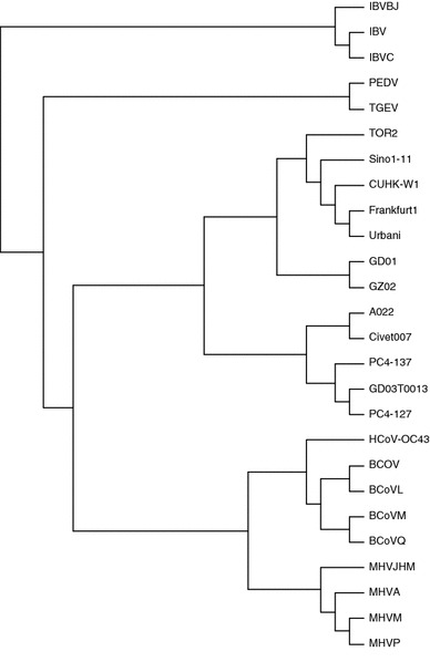
The phylogenetic tree for 26 spike proteins is constructed based on our method HCS(A, B). The proteomic sequence is a concatenation of all the known amino acid sequences for an organism, also with delimiters. Our phylogenetic tree can be obtained at any ionic strength, temperature, time

From Fig. 3, we can see that the phylogenetic tree constructed by our method is more consistent with the known fact of evolution [52]:

1. As can be seen from Fig. 3, SARS-CoVs appear to cluster together and form a new separate branch, which are not closely related to any groups.

2. In respect to HCoV-OC43 , our result in Fig. 3 is same to the result of Yang et al. [52]. That shows our result is more closed to classical results.

Conclusion

With fast development of worldwide genome sequencing project, more and more biological sequences have become available. However, traditional sequence alignment tools and regular evolutionary models are impossible to deal with large-scale protein sequence. Alignment-free method is therefore of great value as it reduces the technical constraints of alignment.

In the present study, we propose a novel alignment-free method, the harmonic common substring measure, for phylogenetic reconstruction based on protein sequences. As it is well known that the more similar two sequences are, the greater the number of the factors shared by the two sequences. So the main advantage is that this algorithm can extract more information hidden in common subsequences. Our examples have indicated that our method is at least as good, and usually better, than some of existing alignment-free methods, both in terms of reconstruction accuracy and of computational efficiency.

Abbreviations

ACS

Average length of longest common substring measure

HCS

Harmonic common substring measure

TF

Transferrin proteins

LF

Lactoferrin proteins

HCS^A_i

The harmonic distribution about all lengths of common substring starting at position i in A

EHCS^A_i

The expectation of HCS ^A_i

References

- 1.Cao Z, Liao B, Li R. Int J Quantum Chem. 2008;108:1485–1490. doi: 10.1002/qua.21698. [DOI] [Google Scholar]
- 2.Chang G, Wang T. J Biomol Struct Dyn. 2011;4:545–555. doi: 10.1080/07391102.2011.10508594. [DOI] [PubMed] [Google Scholar]
- 3.Cover TM, Thomas JA (1991) In: Elements of information theory. Wiley, New York
- 4.Dai Q, Liu X, Wang T. J Mol Struct. 2007;803:115–122. [Google Scholar]
- 5.Dai Q, Yang Y, Wang T. Bioinformatics. 2008;24:2296–2302. doi: 10.1093/bioinformatics/btn436. [DOI] [PubMed] [Google Scholar]
- 6.Felsenstein J. Cladistics. 1989;5:164–166. [Google Scholar]
- 7.Ford M. Mol Biol Evol. 2001;18:639–647. doi: 10.1093/oxfordjournals.molbev.a003844. [DOI] [PubMed] [Google Scholar]
- 8.Guyon F, Brochier-Armanet C, Guénoche A. Adv Data Anal Classif. 2009;3:95–108. doi: 10.1007/s11634-009-0041-z. [DOI] [Google Scholar]
- 9.Hamori E, Ruskin J. J Biol Chem. 1983;258:1318–1327. [PubMed] [Google Scholar]
- 10.Hao B, Qi J (2003) In: Proceedings of the 2003 IEEE bioinformatics conference (CSB 2003), pp 375–385
- 11.Jako E, Ari E, Ittzes P, Horvath A, Podani J. Mol Phys Evol. 2009;52:887–897. doi: 10.1016/j.ympev.2009.04.019. [DOI] [PubMed] [Google Scholar]
- 12.Jeffrey H. Nucleic Acid Res. 1990;18:2163–2170. doi: 10.1093/nar/18.8.2163. [DOI] [PMC free article] [PubMed] [Google Scholar]
- 13.Jia C, Liu T, Zhang X, Fu H, Yang Q. J Biomol Struct Dyn. 2009;6:26–32. doi: 10.1080/07391102.2009.10507288. [DOI] [PubMed] [Google Scholar]
- 14.Jun SR, . Sims GE, Wu GA, Kim SH. Proc Natl Acad Sci. 2010;107:133–138. doi: 10.1073/pnas.0913033107. [DOI] [PMC free article] [PubMed] [Google Scholar]
- 15.Komatsu K, Zhu S, Fushimi H, Qui TK, Cai S, Kadota S. Planta Med. 2001;67:461–465. doi: 10.1055/s-2001-15821. [DOI] [PubMed] [Google Scholar]
- 16.Lempel A, Ziv J. IEEE Trans Inform Theory. 1976;22:75–81. doi: 10.1109/TIT.1976.1055501. [DOI] [Google Scholar]
- 17.Li B, Li Y, He H. Genome Prot Bioinfo. 2005;3:206–212. [Google Scholar]
- 18.Li M, Vitanyi P (1997) In: An introduction to Kolmogorov complexity and its applications. Springer, New York
- 19.Li W, Fang W, Ling L, Wang J, Xuan Z, Chen R. J Biol Phy. 2002;28:439–447. doi: 10.1023/A:1020316706928. [DOI] [PMC free article] [PubMed] [Google Scholar]
- 20.Liao B, Liu Y, Li R, Zhu W. Chem Phys Lett. 2006;421:313–318. doi: 10.1016/j.cplett.2006.01.030. [DOI] [PMC free article] [PubMed] [Google Scholar]
- 21.Liao B, Shan X, Zhu W, Li R. Chem Phys Lett. 2006;422:282–288. doi: 10.1016/j.cplett.2006.02.081. [DOI] [PMC free article] [PubMed] [Google Scholar]
- 22.Liao B, Xiang X, Zhu W. J Comput Chem. 2006;27:1196–1202. doi: 10.1002/jcc.20439. [DOI] [PMC free article] [PubMed] [Google Scholar]
- 23.Lin Y, Fang S, Thorne J. Eur J Oper Res. 2007;176:1908–1917. doi: 10.1016/j.ejor.2005.10.031. [DOI] [Google Scholar]
- 24.Liò P, Goldman N. Trends Microbiol. 2004;12:106–111. doi: 10.1016/j.tim.2004.01.005. [DOI] [PMC free article] [PubMed] [Google Scholar]
- 25.Liu N, Wang T. FEBS Lett. 2006;580:5321–5327. doi: 10.1016/j.febslet.2006.08.086. [DOI] [PubMed] [Google Scholar]
- 26.Liu Y, Yang Y, Wang T. J Biomol Struct Dyn. 2007;25:85–91. doi: 10.1080/07391102.2007.10507158. [DOI] [PubMed] [Google Scholar]
- 27.Liu Z, Liao B, Zhu W. MATCH Commun Math Comput Chem. 2009;61:541–552. [Google Scholar]
- 28.Otu HH, Sayood K. Bioinformatics. 2003;19:2122–2130. doi: 10.1093/bioinformatics/btg295. [DOI] [PubMed] [Google Scholar]
- 29.Ping An He, Yan Ping Zhang, Yu Hua Yao, Yi Fa Tang, Xu Ying Nan. J Comput Chem. 2010;31:2136–2142. doi: 10.1002/jcc.21501. [DOI] [PubMed] [Google Scholar]
- 30.Qi J, Wang B, Hao B. J Mol Evol. 2004;58:1–11. doi: 10.1007/s00239-003-2493-7. [DOI] [PubMed] [Google Scholar]
- 31.Ren F, Tanaka H, Yang Z. Gene. 2009;441:119–125. doi: 10.1016/j.gene.2008.04.002. [DOI] [PubMed] [Google Scholar]
- 32.Randic M, Vracko M, Lers N, Plavsic D. Chem Phys Lett. 2003;368:1–6. doi: 10.1016/S0009-2614(02)01784-0. [DOI] [Google Scholar]
- 33.Randic M, Vracko M, Lers N, Plavsic D. Chem Phys Lett. 2003;371:202–207. doi: 10.1016/S0009-2614(03)00244-6. [DOI] [Google Scholar]
- 34.Randic M, Vracko M, Zupan J, Novic M. Chem Phys Lett. 2003;373:558–562. doi: 10.1016/S0009-2614(03)00639-0. [DOI] [Google Scholar]
- 35.Randic M. Chem Phys Lett. 2004;386:468–471. doi: 10.1016/j.cplett.2004.01.088. [DOI] [Google Scholar]
- 36.Randic M, Zupan J. SAR QSAR Environ Res. 2004;15:191–205. doi: 10.1080/10629360410001697753. [DOI] [PubMed] [Google Scholar]
- 37.Randic M, Lers N, Plavsic D, Basak S, Balaban A. Chem Phys Lett. 2005;407:205–208. doi: 10.1016/j.cplett.2005.03.086. [DOI] [Google Scholar]
- 38.Randic M, Butina D, Zupan J. Chem Phys Lett. 2006;419:528–532. doi: 10.1016/j.cplett.2005.11.091. [DOI] [Google Scholar]
- 39.Randic M, Zupan J, Vikic-Topic D, Plavsic D. Chem Phys Lett. 2006;431:375–379. doi: 10.1016/j.cplett.2006.09.044. [DOI] [Google Scholar]
- 40.Randic M. Acta Chim Slov. 2006;53:477–485. [Google Scholar]
- 41.Randic M. Chem Phys Lett. 2007;444:176–180. doi: 10.1016/j.cplett.2007.06.114. [DOI] [Google Scholar]
- 42.Randic M, Zupan J, Vikic-Topic D. J Mol Graph Model. 2007;26:290–305. doi: 10.1016/j.jmgm.2006.12.006. [DOI] [PubMed] [Google Scholar]
- 43.Randic M, Vracko M, Novic M, Plavsic D. SAR QSAR Environ Res. 2009;20:415–427. doi: 10.1080/10629360903278685. [DOI] [PubMed] [Google Scholar]
- 44.Randic M, Mehulic K, Vukicevic D, Pisanski T, Vikic-Topic D, Plavsic D. J Mol Graph Model. 2009;27:637–641. doi: 10.1016/j.jmgm.2008.10.004. [DOI] [PubMed] [Google Scholar]
- 45.Randic M, Zupan J, Balaban A, Vikic-Topic D, Plavsic D. Chem Rev. 2011;111:790–862. doi: 10.1021/cr800198j. [DOI] [PubMed] [Google Scholar]
- 46.Sims GE, Jun SR, Wu GA, Kim SH. Proc Natl Acad Sci. 2009;106:2677–2682. doi: 10.1073/pnas.0813249106. [DOI] [PMC free article] [PubMed] [Google Scholar]
- 47.Ulitsky I, Burnstein D, Tuller T, Chor B. J Comput Biol. 2006;13:336–350. doi: 10.1089/cmb.2006.13.336. [DOI] [PubMed] [Google Scholar]
- 48.Wang J, Zheng X. Math Biosci. 2008;215:78–83. doi: 10.1016/j.mbs.2008.06.001. [DOI] [PMC free article] [PubMed] [Google Scholar]
- 49.Weiner P (1973) In: Proceedings of 14th IEEE annual symposium on switching and automata theory, pp 1–11
- 50.Wu XM, Cai JP, Wan XF, Hoang T, Geobel R, Lin GH. Bioinformatics. 2007;23:1744–1752. doi: 10.1093/bioinformatics/btm248. [DOI] [PubMed] [Google Scholar]
- 51.Xu Q, Canutescu A, Wang G, Shapovalov M, Obradovic Z, Dunbrack R. J Mol Biol. 2008;381:487–507. doi: 10.1016/j.jmb.2008.06.002. [DOI] [PMC free article] [PubMed] [Google Scholar]
- 52.Yang AC, Goldberger AL, Peng CK. J Comput Biol. 2005;12:1103–1116. doi: 10.1089/cmb.2005.12.1202. [DOI] [PubMed] [Google Scholar]
- 53.Yang L, Chang G, Zhang X, Wang T. Amino Acids. 2010;39:887–898. doi: 10.1007/s00726-010-0547-x. [DOI] [PubMed] [Google Scholar]
- 54.Yu ZG, Zhou LQ, Anh VV, Chu KH, Long SC, Deng JQ. J Mol Evol. 2005;60:538–545. doi: 10.1007/s00239-004-0255-9. [DOI] [PubMed] [Google Scholar]
- 55.Zhang H, Zhong Y, Hao B, Gu X. Gene. 2009;441:163–168. doi: 10.1016/j.gene.2008.07.008. [DOI] [PubMed] [Google Scholar]
- 56.Zhang S, Wang T. MATCH Commun Math Comput Chem. 2010;61:701–716. [Google Scholar]
- 57.Zhang S, Yang L, Wang T. J Mol Struct. 2009;909:102–106. [Google Scholar]
- 58.Zhu W, Liao B, Li R. MATCH Commun Math Comput Chem. 2010;63:483–492. [Google Scholar]