Fitting Nonstationary General-Time-Reversible Models to Obtain Edge-Lengths and Frequencies for the Barry–Hartigan Model

Abstract

Among models of nucleotide evolution, the Barry and Hartigan (BH) model (also known as the General Markov Model) is very flexible as it allows separate arbitrary substitution matrices along edges. For a given tree, the estimates of the BH model are a set of joint probability matrices, each giving the pairwise frequencies of nucleotides at the ends of the edge. We have previously shown that, due to an identifiability problem, these cannot be expected to consistently estimate the actual pairwise frequencies. A further consequence is that internal node frequency estimates are likely to be incorrect. Here we define a nonstationary GTR model for each edge that we refer to as the NSGTR model. We fit the NSGTR model by minimizing the sums of squares between the estimates of transition probabilities under the NSGTR model and the estimates provided by a fitted BH model. This NSGTR model provides estimates that avoid the identifiability difficulties of the BH model while closely fitting it. With the best-fitting NSGTR estimates, we are able to get interpretable frequency vectors at internal nodes as well as edge length estimates that are otherwise not yielded by the BH model. These edge lengths are interpretable as the expected number of substitutions along an edge for the model. We also show that for a nonstationary continuous-time model these are not the same as the edge length parameters for conventional substitution matrices that are output by nonstationary model phylogenetic estimation programs such as nhPhyML.

The time-reversible Markov model assumes a continuous-time stationary process of nucleotide substitution occurs over the tree and is often used in phylogenetic estimation (see Chapter 13 in Felsenstein 2004). For this model, the evolutionary processes are at equilibrium and therefore the root position is not important as the entire topology shares one stationary frequency vector and one substitution rate matrix. The equilibrium assumption is restrictive and violations of this assumption for real data sets have been demonstrated by a number of studies including Yang and Roberts (1995), Foster and Hickey (1999), Foster (2004) and Ababneh et al. (2006). Two commonly used nonstationary models have been proposed in Yang and Roberts (1995) and Galtier and Gouy (1998). Yang and Robert's (YR) model used the Hasegawa-Kishino-Yano (HKY) model proposed in Hasegawa et al. (1985) as the base model, but allowed each edge to have its own edge length and stationary frequency vector. However, in this case the entire tree still shares the same transition and transversion ratio. Galtier and Gouy (1998) suggested a simpler model (the GG model) that allows G+C-content to change throughout the tree. It uses the model in Tamura (1992) as a base and assumes a common transition and transversion ratio along all edges. This model is a special case of the YR model; for each edge, the GG model has two parameters less than the YR model. Compared with these two nonstationary models, the model in Barry and Hartigan (1987) is much more flexible.

The general Markov phylogenetic model first introduced by Barry and Hartigan (1987), known as the BH model, is one of the most flexible models currently available. As with most models, it assumes an independent and identical distribution among sites but differs in that it allows separate arbitrary substitution matrices along edges that need not correspond to a continuous-time Markov process. Work by Jayaswal et al. (2005) and Oscamou et al. (2008) have shown that this model has better phylogenetic estimation properties than simple models when evolutionary processes are nonstationary. However, we previously showed that the estimates of the BH model suffer from identifiability problems that lead to difficulties with correctly estimating internal node frequencies (Zou et al. 2011). A further complication is that the BH model does not directly involve edge length estimation and thus neither conclusions nor subsequent analyses (e.g., molecular clock estimation) can be made that require such information.

A model can be described as nonidentifiable when two or more distinct parameter settings yield the same probability distribution on the data. The maximum likelihood (ML) estimates of a BH model are joint probability matrices. When using the BH model to reanalyze a recently published multigene data set from the malaria parasites of the genus Plasmodium described in Davalos and Perkins (2008), we found that permuting the rows of some of the joint probability matrices gave exactly the same likelihood. Lemma 4.1 of Chang (1996) states that in a three-taxon tree, if the conditional probability matrix is reconstructible from rows, the full model is identifiable. This restriction does not hold for the BH model. Our observations from the Plasmodium data set confirmed that the estimates of transition matrices of the BH model are not unique and there are always at least 24 ML estimates. This differs significantly from the general time reversible (GTR) model because, as shown by Allman et al. (2008), this model with four states is identifiable for all parameters. For the BH model, although the estimates of leaf node state frequencies match the observed frequencies for the corresponding taxa (Jayaswal et al. 2005), there is no guarantee that the estimates of nucleotide frequencies at the internal nodes will be fitted to the right permutations. In this article, we define the best-fitting nonstationary GTR models along edges, referred to as nonstationary best-fit GTR (NSGTR) models, and propose a method that employs the sum of squared differences between NSGTR estimates and BH estimates to identify the estimates of permutations.

The edge length is a useful and informative parameter in phylogenetic analysis that is missing from the BH modeling framework. Although edge lengths were not the primary focus of Jayaswal et al. (2005), ideas were provided for estimating them. In most stationary models, edge lengths are interpretable as the expected numbers of substitutions. This interpretation is desirable for nonstationary models as well but does not apply for some current implementations. Jayaswal et al. (2005) estimated approximate edge lengths for the BH model by averaging the GTR distances for the two opposing evolutionary directions. However, this solution is difficult to justify if the process is nonstationary. Yang and Roberts (1995) pointed out that for nonstationary evolutionary processes, the base frequency vector of an edge will often change along the lineages. The edge lengths in Yang and Roberts (1995) and Galtier and Gouy (1998) were the conventional edge length t^s in P(t^s)=e^Rts for an edge where ∑_j π^s_j R_jj=1, π^s_j is the stationary base frequency and R is the rate matrix. Here superscript s indicates parameters of a stationary model which need not match up with those of a nonstationary model if the frequencies at time 0 differ from the stationary frequencies π^s, for instance. Because both of the YR and GG models are nonstationary, the edge length parameters they employ do not correspond to the conventional interpretation as the expected number of substitutions per site. Fortunately, Minin and Suchard (2008) recently introduced a method to compute the conditional expected number of substitutions in the interval [0, t). This method can be used to obtain edge lengths interpretable as the expected numbers of substitutions per site for the YR, GG, and NSGTR models.

The BH model is particularly valuable when evolutionary processes are nonstationary. However, it suffers from the lack of identifiable internal node frequencies and does not directly provide edge length parameters both of which can be useful to researchers. Here we present methods that allow internal node frequencies and edge length estimates to be obtained from a phylogenetic analysis that utilizes the BH model. The methods introduced here utilize some of the computational advantages of the BH model relative to ML fitting of continuous-time nonstationary models including avoiding computationally expensive repeated eigen decompositions. Our methods complement rather than replace the BH model methodology which, with its greater flexibility, may, in some cases, be able to model some types of processes that no nonstationary continuous-time model could. Example applications we envision include using BH to obtain a tree estimate which is then supplemented with NSGTR edge lengths and frequencies. Alternatively, large differences between NSGTR and BH fits might be used to diagnose unusual evolutionary behavior.

Materials and Methods

The BH model assumes that the evolutionary processes at all sites are independent and share a constant rate (there is no rates-across-sites variation in the model), and that a Markov process of substitution occurs along each edge. This process, however, need not correspond to a continuous-time Markov process. What is required is only that substitutions along an edge (a, b) occur with probabilities given by a matrix P_a,b with positive entries and row sums equal to 1; here P_a,b(i, j) is the probability that nucleotide i at node a is replaced by nucleotide j at node b. Conditional upon the nucleotide at an internal node, the processes along adjacent edges are independent. For instance, for the star tree in Figure 1a, the processes along edges (a, i), (i, b), and (i, c) are independent of each other given the nucleotide at i. The parameters of the joint probability matrices along the edges, may or may not correspond to a continuous Markov chain, but they must satisfy the internal consistency constraint for edges (a, i), (i, b), and (i, c) connected to internal node i whereby state frequencies at node i are the same regardless of the edge matrices. Let F_a,i, F_i,b, and F_i,c denote the BH parameters, joint probability matrices, for edges (a, i), (i, b), and (i, c); F_a,i(j, k) is the probability that nucleotide j is observed at node a and nucleotide k at node i. Using the BH parameters, joint probability matrices F_a,i, F_i,b, and F_i,c, and the frequency π_jⁱ for nucleotide j at node i, the likelihood of a site pattern x={x_a, x_b, x_c} in Figure 1a is

(1)

Because the site likelihood in (1) does not depend upon a root node, while the model is nonstationary, it is root-independent. Equation (1) can be extended to a n-taxon tree. Generally, a root is not required for the BH model.

Figure 1.

Trees of three and four taxa. a) Three taxa; b) four taxa.

In contrast, the NSGTR model described below is a nonstationary model that requires a root for its specification. The model assumes GTR substitution processes along edges away from the root node. However, these GTR substitution processes are allowed to be different for different edges. In addition, the frequencies at the root node need not be the stationary frequencies of a GTR model for an edge connected to the root.

Let denote the BH estimate of the substitution matrix for edge (a, b) and let denote substitution matrix after a permutation σ of either its rows, columns or possibly both. For the NSGTR model, we denote the estimates of the instantaneous rate matrix, the diagonal matrix of stationary frequencies and the evolutionary distance as and . These give a different estimate of substitution matrix . The and consequently are estimated from as described below. A measure of the fit of to is given by . The sum of squares, SS^σ_b,a is also computed for the reverse direction (b, a) using the same procedure. Our procedure considers all possible locations for a root node although, to simplify calculation, we only allow root nodes to be placed at an internal or terminal node, not midway along an edge. Because we consider all root locations, we first obtain the SS^σs for each edge in both forward and backward directions. Given a root, the total SS is obtained the sum of SS^σs over all edges, for each edge, choosing the direction implied by the root. In our approach, the internal consistency requirement plays an important role in determining the permutations. For instance, considering the three-taxon tree in Figure 1a, internal consistency gives F_a,i^T 1 = F_i,b 1 = F_i,c 1, where 1 is a column vector with ones as its elements. If the row permutation of F_i,b of edge (i, b) is changed, the row permutation of F_i,c and the column permutation of F_a,i should be changed accordingly to satisfy internal consistency.

The Best-Fitting Nonstationary GTR Model

Under the assumptions of the NSGTR model above, for any edge (a, b), using the joint probability matrix F_a,b and the frequency vector π_a=∑_b F_a,b, we can compute a transition matrix , where R_a,b is the instantaneous rate matrix of P_a,b; t^s_a,b is the evolutionary time associated with R_a,b of P_a,b. In Markov chain theory, if the process is at equilibrium, the largest of the eigenvalues is equal to 1 and the corresponding left eigenvector is the stationary frequency vector: π_a,b^s P_a,b=π^s_a,b, where π^s_a,b is the base frequency vector at the equilibrium. Using , we can compute R_a,b t^s_a,b. The GTR model obtained above is the best-fit GTR model along edge (a, b) in the direction a→b. Although there is only one correct direction, it is possible that there will be an R_b,a and t^s_b,a corresponding to a model in the reverse evolutionary direction that gives the same joint probabilities and, a priori, we may not know which is the correct direction. However, in general, R_a,b ≠ R_b,a and t^s_a,b≠t^s_b,a, so knowing the direction of evolution matters and hence specification of a root of the tree will ultimately be necessary (discussed further in more detail).

In any case, when estimating the best-fitting NSGTR model in direction a→b, we first obtain the stationary frequencies Π^s_a,b through eigenvector decomposition of P_a,b=Π_a⁻¹ F_a,b where F_a,b and Π_a come from the BH model; Π_a⁻¹ is the inverse matrix of frequency matrix Π_a at node a. As mentioned above, the row of left eigenvectors of P_a,b corresponding to the largest eigenvalue gives the stationary frequencies up to a normalization factor that is subject to ∑_j π^s_(a,b)j=1. Then we calculate a symmetric joint probability matrix F^s_a,b=(Π^s_a,b Π_a⁻¹ F_a,b+(Π^s_a,b Π_a⁻¹ F_a,b)^T)/2. We calculate a symmetric estimate since this is implied by the corresponding true joint probability matrix for a time-reversible model. Using F^s_a,b and Π_a,b^s, we can then compute the rate matrix and the conventional edge length of the transition matrix P^s_a,b=(Π_a,b^s)⁻¹ F^s_a,b for this edge. The rate matrix and conventional edge length are then estimated as log P^s_a,b through eigenvector decomposition.

Forcing F_a,b^s to be symmetric guarantees a real-valued eigenvector decomposition for P_a,b^s. To see this, note that if F_a,b^s is symmetric, so is [Π_a,b^s]^−1/2 F_a,b^s [Π_a,b^s]^−1/2. Because symmetric matrices always have real-valued eigenvector decompositions of the form V Λ V^T, we have that

(2)

By pre- and post-multiplying (2) by [Π_a,b^s]^−1/2 and [Π_a,b^s]^1/2 we see that the eigenvector decomposition of P_a,b^s=U Λ U⁻¹ is related to the eigenvector decomposition of [Π_a,b^s]^−1/2 F_a,b[Π_a,b^s]^−1/2 through U=[Π_a,b^s]^−1/2 V and U⁻¹=V^T [Π_a,b^s]^1/2.

For permutations that do not give valid rate matrices, some corrections were needed. If P_a,b^s has eigenvector decomposition U Λ U⁻¹, then, up to a constant of proportionality, the rate matrix is estimated as U log [Λ] U⁻¹. In practice, it is possible that some of the eigenvalues in Λ will be negative, making it impossible to take logarithms. In this case, we set the corresponding entries of log[Λ] to a large (in magnitude) negative number. One further correction was to set negative entries of the estimated rate matrix to 0 and then adjust diagonal entries accordingly so that rows of the rate matrix sum to 0.

Iteratively Estimating the Permutations of Frequencies at Internal Nodes

As we have previously shown in Zou et al. (2011), different permutations of the rows of the BH substitution model can yield the same distribution of observed data. To illustrate, assume that (x_a, x_b, x_c) are the character states for species a, b, and c in Figure 1a and that these are each 0 or 1. Assume that π₀ and π₁ are the base character frequencies at the internal node i and that P_0,xa, P_1,xa, P_0,xb, P_1,xb, P_0,xc, and P_1,xc are the elements of transition matrices P_i,a, P_i,b, and P_i,c. Now if the rows of P_i,a, P_i,b, and P_i,c are permuted and π₀ and π₁ are exchanged, then we have π₀^σ=π₁, π₁^σ=π₀, where π₀^σ and π₁^σ are the state frequencies after permuting at node i; P_0,xa^σ=P_1,xa, P_0,xb^σ=P_1,xb, P_0,xc^σ=P_1,xc, and etc., where P_i,j^σ are the ij-th entry in the transition matrices after permuting. Comparing the probabilities of the observed character states we obtain

(3)

The pattern probabilities are the same before and after permuting regardless of the observed character states. Because of this lack of identifiability due to permutation, in a DNA data set, 24 sets of estimates of joint probability matrices could give the same likelihood in the three-taxon tree of Figure 1a. In general, for an internal edge which is connected by two internal nodes, there are 576 permutations of the rows and columns of the joint probability matrix for that edge that will give the same probability of data at two internal nodes; for an edge which is connected to an internal node and a leaf node or the root node, there are 24 permutations of the joint probability matrix for that edge that will give the same probability of data at the internal node.

We introduced a parsimony-like method for estimating the correct permutation of frequencies at internal nodes in Zou et al. (2011). For this method to work the frequency vectors at two adjacent nodes should not be too different. Although we have used this method in the analysis of nonstationary data, it will be valuable to have a method that applies in more complicated and general cases. In the following, we introduce a method which can be used to estimate permutations of internal node frequencies without requiring frequencies at adjacent nodes to be similar.

The method for estimating permutations of interval node frequencies obtains the best-fitting NSGTR model above for each permutation of the BH estimated joint probability matrices. The estimated permutations along all edges are taken as those that give the overall minimum distance between the BH substitution matrices and the NSGTR substitution matrices as measured by the sum of squares of differences between these two sets of matrices.

Using the four-taxon tree shown in Figure 1b, we will illustrate in more detail how the permutations are estimated. Our procedure takes all nodes in the tree as valid rooting positions and examines them one by one. For each rooting position, we assign initial permutations for the joint probability matrices of all edges. Taking node a as the root, we compute the total minimum sum of squares minSS from the bottom of the tree to the root a. We start from the node j. In this subtree, we first fix the row permutation of the joint probability matrix of edge (i, j) and pick a permutation σ_j which gives us min SS_j:

(4)

The index σj is the column permutation of Fij and the row permutation of Fjb and Fjc. Having determined the permutation for j, we move to the node i. Keeping the column permutation of Fij as σj, we determine σi giving min SSi using the same criterion of Equation (4) but applied to the three edges connected to the node i. We calculate the total sum of squares of the first iteration using the SSs obtained for edges (a, i), (i, b), (j, c), (j, d), and (i, j) such as minSS1=SSσiai+SSσiib+SSσjjc+SSσjjd+SSσi,σjij. For the second iteration, σi is the initial row permutation of Fij. With this different initial permutation, we repeat the process to obtain another set of σi and σj and min SS2. Iterations continue as long as min SSm < min SSm−1. The permutation indices σi and σj of the final min SS𝒯 are the estimated permutations of the BH estimates when rooting at node a. For each node in the tree, we repeat the procedure with that node being the root. The σi and σj that minimize SS over all root choices are the estimated permutations of BH estimates. To rapidly search over sets of permutations and roots, we pre-computed the SSa,bσ for all permutations and both evolutionary directions. This computation can be completed quickly since there are 24 possible permutations to consider for terminal edges and 576 for internal edges. Given these values, to obtain an overall SS, the algorithm simply needs to select the appropriate SSa,bσ corresponding to the current set of permutations and rooting being considered.

Defining the Number of Substitutions

For most phylogenetic models, rate matrices are conventionally rescaled so that edge lengths are interpretable as expected numbers of substitutions. For a stationary model, if R is the rate matrix and Π^s the stationary matrix, R is rescaled so that ∑_j π^s_j R_jj=1. For nonstationary models, however, this rescaling will not necessarily give edge lengths with the correct interpretation (Minin and Suchard, 2008). Below we give a formula for the expected number of substitutions under a nonstationary continuous-time Markov model with an unscaled rate matrix.

Let N(t) be the number of substitutions over an edge of length t; let R be the instantaneous rate matrix of a continuous time Markov model; P(t)=e^Rt is the corresponding substitution matrix. Let X_t denote the character state of the process at time t and let R_ℒ denote the rate matrix R but with diagonal entries set to zero. Equation (2.3) of Minin and Suchard (2008) gives

Thus, if β_i=P(X₀=i),

Because ∑_j[e^R(t−z)]_kj=∑_j P_k,j(t−z)=1 and ∑_k≠l R_lk = − R_ll, we obtain that

For a time-reversible model, P(t) has an eigenvector decomposition as P(t)=Ue^Λt U⁻¹ where e^Λt is a diagonal matrix in which the ii-th diagonal entry gives i-th eigenvalue e^λ_it so that one of the λ_i is zero and the rest are negative; the i-th column of U gives the i-th eigenvector of P. Using the eigenvector decomposition

(5)

When j=1, the eigenvalue is zero which is the largest eigenvalue of the rate matrix. Thus ∫^t₀ e^λ₁z dz=t. When j≠1, . Thus,

(6)

Given an edge with substitution matrix P(t)=e^Rt for an unscaled R, if we take our edge length as t^e = 𝔼[N(t)] and rescale R by , then t^e will be interpretable as the expected number substitutions.

If the β_i are the stationary frequencies π^s_i for R, this gives the conventional rescaling where − ∑_j π^s_j R_jj = 1. The edge lengths coming from this rescaling will be denoted t^s and t^s = t^e only in the case of a stationary model. For the NSGTR model, the appropriate β_i required to calculate t^e are the frequencies at the starting node which need not coincide with the stationary frequencies.

Results

Simulation Settings

We used the INDELible sequence simulator (Fletcher and Yang 2009) to create data sets under the GG and BH models to test the performance of our methods. The parameters of interest are joint probability matrices along edges, frequencies at all nodes and edge lengths. In our simulations, we evaluated both “mild” and “extreme” settings for parameters. The mild parameters corresponded to the parameter estimates obtained for the NSGTR model fitted to a real phylogenomic data set consisting of data from the genus Plasmodium (Davalos and Perkins 2008). The extreme parameters had extreme stationary frequencies and exchangeabilities but the same NSGTR edge lengths as in the mild parameters data set. The tree in Figure 1 A in Davalos and Perkins (2008) was treated as the true tree and has been reproduced in Figure 2.

Figure 2.

The tree used in the simulations. In the figure, nodes b, c, f, g, k, r, v, and y represent the taxa of P. berghei, P. chabaudi, P. falciparum, P. gallinaceum, P. knowlesi, P. reichenowi, P. vivax, and P. yoelii.

Estimated Permutations

Our experience suggests that optimization of parameters under the BH model can sometimes yield local maxima. To check whether this was the case in our analysis, for a given data set simulated using the mild parameters setting, we randomly generated 100 sets of joint probability matrices under the true tree as our initial values to seed the optimization. When estimating parameters of the BH model for each of the 100 sets of joint probability matrices, we found that 94 out of the 100 had the same maximum log-likelihood up to one decimal place, −335974.1. In the following, we will ignore the six sets of estimates which had much smaller suboptimal log-likelihoods corresponding to local maxima. For each of the 94 set of estimates, we obtained the best-fitting NSGTR joint probability matrices. The best-fitting NSGTR joint probability matrices for the estimated permutation had much smaller distances between the estimates and true values than the best-fitting NSGTR matrices for other permutations. None of the 94 sets of best-fitting permutations corresponded to the original BH estimates reinforcing our results indicating that BH estimation alone is only accurate up to permutation (Zou et al. 2011).

We performed tests to see if our algorithm can find the set of permutations, over internal nodes, that gives the minimum overall sum of squares. These tests were conducted for 18 simulated data sets under both mild and extreme parameter settings. In each of these cases, and for almost all root choices, the overall minimum sum of squares from our algorithm was the same as the sum of the separately minimized sums of squares for each of the edges. This implies that our algorithm found the global minimum in each case. (Note that any permutation at an internal node implies the permutations of rows or columns of substitution matrices for each of the edges connected to that node. Because separately minimizing sums of squares along edges does not enforce this constraint, it does not give a global minimizer of the overall sum of squares except, as here, when it matches up with a set of permutations that satisfy the constraint.) For any root, the global minimizing permutation was unique. However, except for one of the data sets simulated under extreme settings, the same overall minimum sum of squares was obtained no matter which root was selected.

The results of Zou et al. (2011), reviewed here, established that joint probability matrices for edges can only be identified up to permutation in the BH model. For the NSGTR model, this is no longer the case. As we establish in supplementary material, for a given topology and rooting, all parameters of the NSGTR model are identifiable.

Edge Length Estimation

We compared the parameter estimates obtained from our NSGTR fit to the estimated BH model on the data sets with results estimated under a stationary GTR model using PhyML (Guindon and Gascuel 2003) and the GG nonstationary model implemented in nhPhyML (Boussau and Gouy 2006). Estimated edge lengths from PhyML and nhPhyML are the t^s parameter using the conventional rescaling for stationary models, ∑_j π^s_j R_jj=1, where π is the stationary frequency vector. For the GTR model, this t^s is equivalent to the expected number of substitutions per site. However, for the nonstationary evolutionary processes accommodated by the GG or the BH models along edges, the standard t^s edge length parameter is not the expected number of substitutions; the latter (i.e., t^e) is instead correctly computed using (6). In our experiments, we obtained estimates of the t^s parameter edge lengths from the GTR and GG models using PhyML and nhPhyML. We also computed the estimates of the expected number of substitutions (the t^es) along edges using the estimates of joint probabilities of the GG and NSGTR models in (6). Because this is a simulated data set, we also present the true average numbers of substitutions in Figure 3.

Figure 3.

Estimates of edge lengths for data simulated from four models with extreme parameters.

For the tree in Figure 3, we can separate the edges into two groups: a long edge group containing edges (5, 2), (6, 1), (6, g), and (5, 4) and a short edge group containing edges (1, f), (1, r), (4, c), (3, b), and (3,y). The estimates of edge lengths for the short edge group are very similar across different models and methods for calculating edge lengths. In the long edge group, the NSGTR estimates tend to be the closest to the true edge lengths. The estimates of t output by nhPhyML, t^s, and the expected number of substitutions for this data set, t^e, obtained by correcting the t^s parameter with (6) did much better than the estimates of the GTR model from PhyML. For the GTR model, the estimates for all edges were poor, and especially for edge (6, 5) that was estimated to be zero when its true value was 0.033. Notably, the GTR model estimates stretched all edges in the long edge group. That the GTR model performed worst under these conditions is not surprising given that it was badly misspecified.

By assuming a general reversible continuous-time Markov process for the direction from the root to the terminal nodes along each edge, we can fit the NSGTR models along edges. In this model, the parameters are the root frequencies, exchangeabilities, and stationary frequencies vectors for each edge. Using bppml in the BppSuite in Dutheil and Boussau (2008), we are able to obtain ML parameter estimates for the NSGTR models, referred to as the NSGTR-ML method. We compared the estimates of edge lengths obtained using our method (i.e., fitting the BH model and then finding the best-fit NSGTR models) with those estimated by the NSGTR-ML method. For this comparison, we used an eight-taxon data set simulated under the BH model and the mild parameter settings. For each comparison, we calculated the average difference (in absolute value) between the estimates and the true values. The average differences for edge lengths are 0.022 for our method and 0.030 for the NSGTR-ML method.

We did an additional simulation to explore the effects of edge lengths estimated by nhPhyML under a correctly specified GG model. Using INDELible, we simulated a series of pairs under the GG model with 77313 sites. All pairs had the same starting state frequency vector {0.41, 0.10, 0.16, 0.33} for nucleotides A, C, G, T, G+C-content of 0.9 and transition/transversion ratio parameter 2, but each pair has a unique edge length. The results are presented in Table 1. As can be seen, the estimates of the expected numbers of substitutions t^e are much closer to the true values than the t^s edge lengths output by nhPhyML.

Table 1.

The branch lengths and expected numbers of substitutions in the simulation for testing nhPhyML estimates of branch lengths

ts		te
True*	Estimate*	True**	Estimate**
0.1	0.159	0.115	0.141
0.2	0.293	0.224	0.260
0.3	0.410	0.327	0.361
0.4	0.508	0.426	0.451
0.5	0.624	0.520	0.569
0.6	0.720	0.610	0.630
0.7	0.806	0.697	0.798
0.8	0.909	0.782	0.793
0.9	0.996	0.864	0.880
1.3	1.377	1.176	1.199
1.4	1.472	1.251	1.203
2.0	2.080	1.683	1.333

True^*: branch length in T92 model.

Estimate^*: the estimates of nhPhyML.

True^**: the true expected numbers of substitutions.

Estimate^**: the estimates of the expected numbers of substitutions.

In a nonstationary model, the edge lengths t^s determined by ∑_j π_j^s R_ij=1 are not equal to the edge lengths t^e calculated by (6). Figure 4 shows the differences between t^e and t^s vs. t^s of a pair of taxa. In this set of calculations, we set the root frequencies to {0.4, 0.1, 0.1, 0.4} and created substitution matrices under the T92 model with parameters satisfying that (1) the frequency of nucleotide C is in {0.05, 0.10, 0.15, 0.35, 0.40, 0.45}; (2) the ratio of transition and transversion processes is 4.0; (3) the stationary evolutionary distance is in [0.05, 2.0]. The six plots in Figure 4 showed that when the evolutionary distances are small, the differences between t^e and t^s are small; when the evolutionary distances are large, the differences between t^e and t^s increase. The frequencies of nucleotides also contributed to the size of the difference between t^e and t^s. When the stationary frequencies of nucleotides are close to the root frequencies, which is close to stationary status, the differences between t^e and t^s are small. The smallest difference, zero, happens when the nucleotide's frequencies at root is equal to the stationary frequencies, which indicates the stationary status. Results for other ratios of transition and transversion in [0.5, 5] with the same set of frequencies of nucleotide C and evolutionary distances, which are not presented here, showed similar patterns.

Figure 4.

The differences between expected numbers of substitutions t^e and stationary distance t^s for T92 model. For each plot, the title indicates the stationary frequency of state C in T92 model; the x-axis is the stationary edge lengths t^s in T92 model; the y-axis is the differences between t^s − t^e.

Compositional Heterogeneity

The Plasmodium data set in Davalos and Perkins (2008) has evidence of nonstationarity. The A+T-content in Plasmodium knowlesi and Plasmodium vivax are higher than in others. Also, as shown in Table 2, the frequencies of nucleotides C and G are not similar for taxa P. berghei, P. chabaudi, P. falciparum, P. gallinaceum, P. reichenowi, and P. yoelii.

Table 2.

The character frequencies of eight taxa in Plasmodium data set

	Plasmodium berghei	Plasmodium chabaudi	Plasmodium falciparum	Plasmodium gallinaceum	Plasmodium knowlesi	Plasmodium reichenowi	Plasmodium vivax	Plasmodium yoelii
A	0.41	0.41	0.41	0.41	0.35	0.41	0.32	0.42
C	0.11	0.11	0.11	0.10	0.18	0.11	0.21	0.11
G	0.16	0.16	0.16	0.16	0.21	0.16	0.24	0.16
T	0.32	0.32	0.32	0.32	0.26	0.32	0.23	0.32

We fitted the GTR, GG, NSGTR, and BH models for the Plasmodium data set. The log likelihoods for the GTR, GG, NSGTR-ML, and BH estimates ranged from −348615.7 to −335974.1. As there are 8 taxa in the Plasmodium data set, for a fixed topology, there are 22 free parameters using the GTR model, 30 free parameters in the GG model, 129 free parameters in the NSGTR-ML method, and 159 free parameters in the BH model. The differences of log likelihoods and degrees of freedom between the BH and GTR models are 6320.5 and 137 respectively, the corresponding differences between the BH and GG models are 2446 and 93 respectively, and the same differences between the BH and NSGTR-ML methods are 197 and 30 respectively; likelihood ratio tests clearly reject the simpler models in favor of BH. We compared the estimates of joint probability matrices along edges of the BH and NSGTR-ML methods and obtained 0.011 as the average difference among all entries. Among the entries of joint probability matrices of the BH estimates, the average value is 0.0625. Although the difference in log likelihoods indicates that BH gives a significantly better fit, this significant departure does not seem to correspond to a large departure in estimated parameter values.

The results for node frequencies are given in Figure 5. Up to numerical/optimization error, the BH estimates of terminal node frequencies match the empirical frequencies as was shown analytically in Jayaswal et al. (2005). The NSGTR and BH frequencies are very similar with 10⁻³ as the maximum difference (in absolute value) across all nodes. The average difference of the estimates of the leaf node frequencies between the NSGTR-ML and BH models was 0.031, which is much larger than the maximum difference of 10⁻³ between the estimates of the NSGTR and BH models. Because they are constant, the GTR model estimates are unable to capture the frequency changes over the topology in Figure 5. Because A=T and C=G in the GG model which is clearly not the case at terminal nodes, the GG model did not fit much better than the GTR model except at nodes P. knowlesi and P. vivax. At these two nodes, the frequencies of nucleotides A and T are close.

Figure 5.

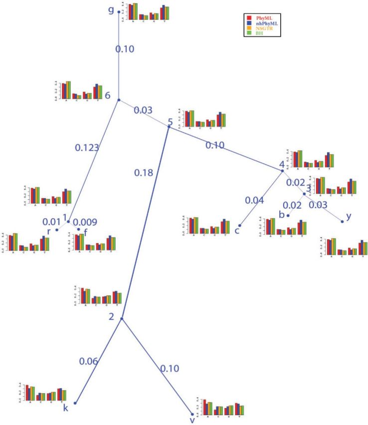
Estimates of frequencies at internal and external nodes for the Plasmodium data set. In the figure, nodes b, c, f, g, k, r, v, and y represent the taxa of P. berghei, P. chabaudi, P. falciparum, P. gallinaceum, P. knowlesi, P. reichenowi, P. vivax, and P. yoelii. In a bar chart for a given nucleotide, bars from left to right give frequencies for PhyML, nhPhyML, NSGTR, and BH respectively.

Normally, a large edge length indicates a large change of frequencies at two nodes. For the real Plasmodium data, the largest edge length estimate is for edge (5, 2). This largest value also corresponds to the largest frequency changes with the average difference 0.069. For other edges, the average differences of frequencies at two end nodes is at most 0.022. The edge (5, 2) separates the taxa k, v from the others. Figure 5 also showed that the NSGTR estimates do well at fitting the changes in frequencies; the NSGTR-ML and nhPhyML estimates also had the largest change along edge (5, 2), but their estimates are not as close due to the restriction of the stationary assumption in the NSGTR-ML model and the GG model restriction that frequencies of states C and G be the same. Because there is only one frequency vector for the entire topology, unsurprisingly, PhyML was unable to accurately estimate the frequencies for nodes k, v, and 2.

The results for the simulated data set in Figure 6 show a more complex example with extreme parameters models along edges. In the true model, node g, which is the root when estimating BH estimates, has a high A+T-content with nucleotide A having the highest frequency. The cluster of nodes 1, k, and r have high G+C-content with nucleotide C having the highest frequency. The cluster of nodes 2, k and v have roughly equal A+T-content and G+C-content with nucleotide G having the highest frequency. Finally, the cluster of nodes 4, c, 3, b, and y have high A+T-content with nucleotide T having the highest frequency. The estimates of the BH under the estimated permutations were within 10⁻⁴ of simulated values.

Figure 6.

Estimates of frequencies at internal and external nodes for simulated data from a model with extreme parameters. In a bar chart for a given nucleotide, bars from left to right give frequencies for PhyML, nhPhyML, NSGTR, and true values, respectively.

Similar to the observed results for the Plasmodium data, large changes in frequency vectors are expected over longer evolutionary times. When the edge lengths are small, the frequency vector did not change much. For instance, the average difference between the frequency vectors at nodes 1 and f is 0.0056 over an edge of length 0.02. In contrast, the average difference between the frequency vectors at nodes g and f is 0.18 over an edge of length 0.62 for the simulated data set with extreme parameters. The estimates of the NSGTR-ML and nhPhyML models showed a similar pattern, with the frequency vector changes being largest along the longest edge. Again, estimates from PhyML could not accommodate the changing frequencies.

Discussion

Our NSGTR implementation is intended to supplement a BH model analysis, which is a more flexible nonstationary model, by providing edge lengths and internal node frequencies that, in most cases, are meaningful. If one was only interested in NSGTR model fits, it could be directly fit in an ML framework and this would, in theory, provide parameter estimates with smaller variance. We used the methods described in Dutheil and Boussau (2008) to obtain such fits for the data and simulations considered here. Alternatively, Jayaswal et al. (2011) recently provided an R implementation allowing model selection over continuous-time reversible models with varying degrees of heterogeneity. Our results for the data and simulations considered here suggest that our NSGTR fits will be comparable with NSGTR-ML. In fact, for the comparisons here, our parameter estimates were closer to the true generating parameters in some cases. Due to the statistical consistency of the BH joint probability matrix estimates, our approach can be expected to give statistically consistent estimates of NSGTR parameters.

Surprisingly, the total computational time required to fit both the BH and the NSGTR models was much less than the time required for a single NSGTR-ML fit. The total time required for both BH and NSGTR fits to the Plasmodium data set was <2 min where for this data, the time required for NSGTR-ML fitting was >1 h. The reason for the shorter time has much to do with the computational advantages of the BH model implementation. Jayaswal et al. (2005) provide explicit updating formulas that do not require eigenvector decompositions. In our experience, estimation can be done quickly. In contrast, an NSGTR ML implementation requires repeated eigenvector decompositions through all edges of a tree, every time new NSGTR parameters are considered as well as when derivatives of these parameters are required.

The stationary GTR model has a closure property: if one taxon is taken out, the implied model for the remaining taxa is a GTR model. For the NSGTR model, if one taxon is taken out, the implied model will be approximately NSGTR if the rate matrices do not change much near the terminal branch for that taxon. Results in Sumner et al. (2012) imply that the NSGTR is not generally closed, however. Thus, for the NSGTR model to give a good fit, it is important that taxon sampling be conducted in such a way that, for any given edge, a single GTR model provides a reasonable approximation to the evolutionary process along that edge.

When edge lengths are short, the estimates from GTR, GG, and NSGTR are quite similar. However, when an edge length was large, NSGTR estimates tended to estimate the changes of frequencies and edge lengths much better than the alternative methods. For the Plasmodium data set shown in Figure 7, the edge lengths output from GTR and GG are not very different from expected numbers of the substitutions obtained using (6) and the estimates of NSGTR model. This is not surprising for this particular data set because the NSGTR estimates of parameters for this data set indicated that exchangeabilities and stationary frequencies did not change much over the tree except at the edge (5, 2). The processes along most edges are, therefore, close to being stationary processes. However, our simulation study under more extreme nonstationary parameter settings clearly shows the improved accuracy of the NSGTR method relative to the GG and GTR models.

Figure 7.

Estimates of edge lengths for the Plasmodium data under four different models. In the figure, nodes b, c, f, g, k, r, v, and y represent the taxa of P. berghei, P. chabaudi, P. falciparum, P. gallinaceum, P. knowlesi, P. reichenowi, P. vivax, and P. yoelii.

While the NSGTR model estimated many parameters well, it did not do a good job at locating the root. Evaluating the minSS values rooting at different nodes of Plasmodium data set yielded two distinct values. Rooting at the nodes 1, 3, 4, 5, 6, b, c, f, g, r, and y gave a minSS value of approximately 2.34E − 04, whereas rooting at the nodes 2, k, and v gave a minSS value of approximately 1.48E − 03. This difference in minSS allows us to rule out node 2, k, and v as the true root but does not distinguish between the others.

One of the pragmatic decisions made in fitting was to only consider internal or external nodes as potential roots. Allowing roots along an edge may seem desirable by comparison but comes with the additional complication of optimizing the location along that edge. For the examples considered here, because of the small SS obtained between BH and NSGTR, it is doubtful that substantial further decreases would be obtained via the additional flexibility of allowing a root anywhere along an edge. More generally, since by comparison with our current implementation allowing a root along an edge will only change the fit for that one edge, it is doubtful that such additional flexibility will appreciably improve fit.

To explain our observations, we obtained the NSGTR substitution matrices for one of the rootings giving the minimum minSS. These NSGTR substitution matrices were used to obtain joint probability matrices, which were given as input to the NSGTR routine. We used this routine to compute NSGTR models from true joint probabilities in the reverse directions along edges. We found that the true joint probability matrices coming from NSGTR in the reverse direction were almost identical (data not shown). Based upon these numerical results, it appears that the evolutionary direction for an edge under the NSGTR model is not always recoverable. For the Plasmodium data set, the estimates of edge lengths of the forward and reverse directions show few differences. However for the case of extreme data sets in our simulation, the direction effects were significant.

A natural follow-up question is whether there always exists an NSGTR model in the reverse direction if there exists a NSGTR model in the forward direction. We tested 18 data sets simulated under GTR models and BH models and obtained BH estimates. For each set of BH estimates, we examined 14 rooting positions. Among a total of 18*14=252 rooting trials, we only had two cases in which NSGTR models did not give exactly the same fit in both forward and backward directions.

Finally, it should be pointed out that there may be cases where the fitted BH model is not well-approximated by any NSGTR model. In this case, the resulting edge lengths from NSGTR could be misleading. Such cases can be expected to be diagnosed through large differences between NSGTR and BH model substitution matrices.

Conclusions

The parameters of the BH model of Barry and Hartigan (1987) are joint probabilities along edges and they have identifiability problems whereby multiple sets of estimates give the same likelihoods. Because of this, frequencies at internal nodes cannot be correctly estimated although frequencies at leaf nodes will converge to true values as sequence length gets large. A further problem is that edge lengths are informative parameters but are not available from the BH model. By defining NSGTR models along edges, our algorithm finds the estimates of the transition matrices under the NSGTR model that best fits the BH estimates. Our simulations show that our algorithm is effective in resolving identifiability problems in both mild and extreme parameter settings.

In our solution, because the NSGTR model is nonstationary, nonstandard methods were required to compute the edge length interpretable as the expected number of substitutions along an edge. Our approach of using NSGTR estimates of the best-fitting BH estimates allows interpretable edge lengths to be estimated. The formulas given for edge length calculation are more broadly valuable for obtaining interpretable edge lengths for all nonstationary models. For instance, the estimates of edge lengths currently given by the nhPhyML implementation of the GG model correspond to stationary model calculations but can be corrected using (6).

Software implementing the methods discussed in this article is available at http://www.mathstat.dal.ca/~tsusko.

Funding

This work was supported by Discovery grants from the Natural Sciences and Engineering Research Council of Canada awarded to C.F., E.S., and A.J.R.

References

- Ababneh F., Jermiin L.S., Ma C., Robinson J. Matched-pairs tests of homogeneity with applications to homologous nucleotide sequences. Bioinformatics. 2006;22:1225–1231. doi: 10.1093/bioinformatics/btl064. [DOI] [PubMed] [Google Scholar]
- Allman E., Ane C., Rhodes J.A. Identifiability of a Markovian model of molecular evolution with gamma-distributed rates. Adv. Appl. Prob. 2008;40:229–249. [Google Scholar]
- Barry D., Hartigan J.A. Statistical analysis of hominoid molecular evolution. Stat. Sci. 1987;2:191–210. [Google Scholar]
- Boussau B., Gouy M. Efficient likelihood computations with nonreversible models of evolution. Syst. Biol. 2006;55:756–768. doi: 10.1080/10635150600975218. [DOI] [PubMed] [Google Scholar]
- Chang J.T. Full reconstruction of Markov models on evolutionary trees: identifiability and consistency. Math. Biosci. 1996;137:51–73. doi: 10.1016/s0025-5564(96)00075-2. [DOI] [PubMed] [Google Scholar]
- Davalos L.M., Perkins S.L. Saturation and base composition bias explain phylogenomic conflict inPlasmodium. Genomics. 2008;91:433–442. doi: 10.1016/j.ygeno.2008.01.006. [DOI] [PubMed] [Google Scholar]
- Dutheil J., Boussau B. Non-homogeneous models of sequence evolution in the Bio++ suite of libraries and programs. BMC Evol. Biol. 2008;8:255. doi: 10.1186/1471-2148-8-255. [DOI] [PMC free article] [PubMed] [Google Scholar]
- Felsenstein J. Inferring phylogenies. Sunderland Massachuetts (MA): Sinauer Associates, Inc; 2004. [Google Scholar]
- Fletcher W., Yang Z. INDELible: a flexible simulator of biological sequence evolution. Mol. Biol. E. 2009;26:1879–1888. doi: 10.1093/molbev/msp098. [DOI] [PMC free article] [PubMed] [Google Scholar]
- Foster P.G. Modeling compositional heterogeneity. Syst. Biol. 2004;53:485–495. doi: 10.1080/10635150490445779. [DOI] [PubMed] [Google Scholar]
- Foster P.G., Hickey D.A. Compositional bias may affect both DNA-based and protein-based phylogenetic reconstructions. J. Mol. Evol. 1999;48:284–290. doi: 10.1007/pl00006471. [DOI] [PubMed] [Google Scholar]
- Galtier N., Gouy M. Inferring pattern and process: maximum-likelihood implementation of a nonhomogeneous model of DNA sequence evolution for phylogenetic analysis. Mol. Biol. Evol. 1998;15:871–879. doi: 10.1093/oxfordjournals.molbev.a025991. [DOI] [PubMed] [Google Scholar]
- Guindon S., Gascuel O. A simple, fast, and accurate algorithm to estimate large phylogenies by maximum likelihood. Syst. Biol. 2003;52:696–704. doi: 10.1080/10635150390235520. [DOI] [PubMed] [Google Scholar]
- Hasegawa M., Kishino H., Yano T. Dating of the human-ape splitting by a molecular clock of mitochondrial DNA. J. Mol. Evol. 1985;22:160–174. doi: 10.1007/BF02101694. [DOI] [PubMed] [Google Scholar]
- Jayaswal V., Jermiin L., Robinson J. Estimation of phylogeny using a general Markov model. Evol. Bioinf. Online. 2005;1:62–80. [PMC free article] [PubMed] [Google Scholar]
- Jayaswal V., Jermiin L.S., Poladian L., Robinson J. Two stationary nonhomogeneous markov models of nucleotide sequence evolution. Syst. Biol. 2011;60:74–86. doi: 10.1093/sysbio/syq076. [DOI] [PubMed] [Google Scholar]
- Minin V.N., Suchard M.A. Fast, accurate and simulation-free stochastic mapping. Philos. Trans. R. Soc. Lond. B. Biol. Sci. 2008;363:3985–3995. doi: 10.1098/rstb.2008.0176. [DOI] [PMC free article] [PubMed] [Google Scholar]
- Oscamou M., McDonald D., Yap V.B., Huttley G.A., Lladser M.E., Knight R. Comparison of methods for estimating the nucleotide substitution matrix. BMC Bioinformatics. 2008;9:511. doi: 10.1186/1471-2105-9-511. [DOI] [PMC free article] [PubMed] [Google Scholar]
- Sumner J.G., Fernández-Sánchez J., Jarvis P.D. Lie markov models. J. Theor. Biol. 2012;298:16–31. doi: 10.1016/j.jtbi.2011.12.017. [DOI] [PubMed] [Google Scholar]
- Tamura K. Estimation of the number of nucleotide substitutions when there are strong transition-transversion and G+C-content biases. Mol. Biol. Evol. 1992;9:678–687. doi: 10.1093/oxfordjournals.molbev.a040752. [DOI] [PubMed] [Google Scholar]
- Yang Z., Roberts D. On the use of nucleic acid sequences to infer early branchings in the tree of life. Mol. Biol. Evol. 1995;12:451–458. doi: 10.1093/oxfordjournals.molbev.a040220. [DOI] [PubMed] [Google Scholar]
- Zou L., Susko E., Field C., Roger A.J. The parameters of the Barry and Hartigan general Markov model are statistically nonidentifiable. Syst. Biol. 2011;60:872–875. doi: 10.1093/sysbio/syr034. [DOI] [PubMed] [Google Scholar]