Multi-core CPU or GPU-accelerated Multiscale Modeling for Biomolecular Complexes

Abstract

Multi-scale modeling plays an important role in understanding the structure and biological functionalities of large biomolecular complexes. In this paper, we present an efficient computational framework to construct multi-scale models from atomic resolution data in the Protein Data Bank (PDB), which is accelerated by multi-core CPU and programmable Graphics Processing Units (GPU). A multi-level summation of Gaus-sian kernel functions is employed to generate implicit models for biomolecules. The coefficients in the summation are designed as functions of the structure indices, which specify the structures at a certain level and enable a local resolution control on the biomolecular surface. A method called neighboring search is adopted to locate the grid points close to the expected biomolecular surface, and reduce the number of grids to be analyzed. For a specific grid point, a KD-tree or bounding volume hierarchy is applied to search for the atoms contributing to its density computation, and faraway atoms are ignored due to the decay of Gaussian kernel functions. In addition to density map construction, three modes are also employed and compared during mesh generation and quality improvement to generate high quality tetrahedral meshes: CPU sequential, multi-core CPU parallel and GPU parallel. We have applied our algorithm to several large proteins and obtained good results.

1. Introduction

Finite Element Analysis has been essentially important for the study of biomolecular complexes in a wide range of applications such as estimating electrostatic potentials and diffusion-based calcium signaling [9, 17, 20, 40, 41, 47, 49]. As progressively larger biomolecular complexes (see Fig. 1) are studied, we need to handle huge amount of computation, which brings a great challenge for both modeling and simulation. To efficiently represent complex biomolecules, a multiscale modeling method that controls the local resolution of the specified hierarchical structure is required, which can significantly reduce the mesh size and thus lighten the compuational cost for simulations. In addition, with the rapid development of parallel computers, multi-core CPU and GPU-based computation brings in new directions for the acceleration of modeling in various fields. In this paper we aim to apply these parallel computation techniques to multiscale modeling for biomolecules. In the following, let us first briefly review previous work on biomolecular modeling and efficient computation.

Fig 1.

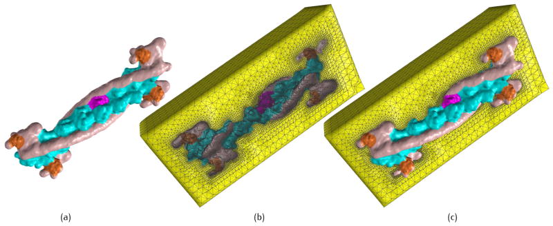
Multi-scale model for the thin filament complex (TFC, PDB ID: 2W4U). High resolution is shown for the actin domain (cyan) with parameters P_R = 0.8, P_C = 0.5, and P_D = 1.0; chain K (magenta) and troponin C (orange) are further emphasized with P_R = 2.0, P_C = 1.0, and P_D = 1.0; and the rest of the protein (pink) is blurred with P_R = 0.5, P_C = 0.3, and P_D = 0.8. (a) Biomolecular surface; (b) exterior tetrahedral mesh; and (c) exterior mesh with embeded protein. P_R, P_C and P_D are parameters to control the local resolution of residuals, chains and domains, respectively.

There are three important biomolecular surfaces [10, 11]: the Van der Waals surface (VdW), the Solvent Accessible Surface (SAS), and the Solvent Excluded Surface (SES). For the VdW, atoms are represented as rigid spheres with Van der Waals radii, and the biomolecular surface is defined as the envelope of these spherical surfaces. The SAS and SES can be defined by assuming a probe rolling around the biomolecule and keeping contact with the atoms. Then the SAS is formed by tracing the trajectory of the probe center. The topological boundary of the union of all possible probes is called the SES, with no intersection with atoms. A lot of research has been conducted in approximating the SES, including the the alpha-shapes [1, 13], the beta-shapes [26, 36], the MSMS [37], the advancing front and generalized Delaunay approaches [27], NURBS approximation [6], and PDE-based methods [21, 46, 53]. The biomolecules were also represented as implicit models. The Gaussian kernel functions were applied in constructing density maps for the biomolecules [8, 19, 28, 48, 52]. In [18], the atomic resolution Gaussian density map was built and then filtered using an ideal filter to obtain a smooth biomolecular surface.

Fast computing is critical in biomolecular modeling [43, 45]. A variety of algorithms were developed in improving the modeling efficiency. For example, the Fast Fourier Transform was used in [21, 53] to get better performance of the PDE transform, and a Non-uniform Fast Fourier Transform (NFFT) was adopted to improve the polynomial-form summation of the kernel functions [7]. The programmable GPU has brought in a new direction for vast data processing in geometric modeling [24, 30, 35, 42, 44].

In this paper, we propose an efficient multi-scale modeling framework for biomolecules based on the multi-level summation of Gaussian kernel functions. The modeling process contains three steps: Gaussian density computation, adaptive tetrahedral mesh generation, and quality improvement. A special method called neighboring search is applied for efficiency improvement, together with the KD-tree structure and the bounding volume hierarchy (BVH). The multi-core CPU and GPU-based parallel computation techniques are employed in all these three steps. The main contributions in this paper include:

1. Structure specified parameters are adopted in the multi-level summation of Gaussian kernel functions, enabling a local resolution control for the hierarchical structure of the complicated biomolecules;

2. Neighboring search is applied to locate the grid points close to the biomolecular surface, and thus reduce the number of grids to be analyzed;

3. KD-tree and BVH are employed to quickly search contributing atoms around a grid point. Faraway atoms are ignored due to the decay of Gaussian kernel functions; and

4. Multi-core CPU and GPU-based computation are employed in the entire modeling process, which significantly accelerate the modeling process.

The remainder of this paper is organized as follows. Section 2 describes the multi-level summation of Gaussian kernel functions. Section 3 explains the Gaussian density map construction, promoted by the neighboring search, KD-tree structure, BVH, and parallel computation. Sections 4 and 5 talk about mesh generation and quality improvement, respectively. Section 6 shows the results. Finally, section 7 draws conclusions and points out the future work.

2. Multi-scale Biomolecular Modeling

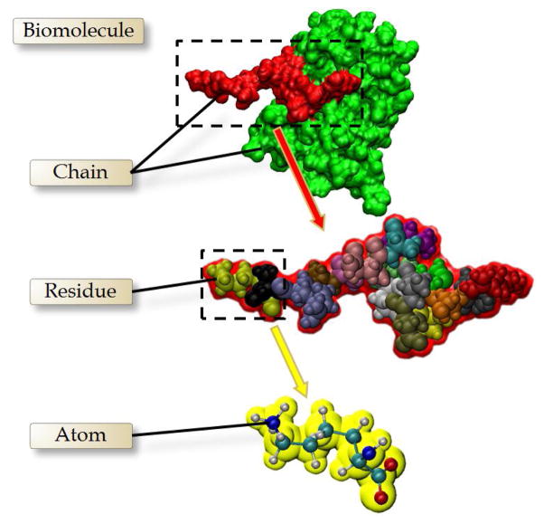
As shown in Fig. 2, biomolecules usually have a complicated hierarchical structure, including the atomic, residual, and chain scales. A variety of methods have been developed to create multi-resolution models for the biomolecules [5, 18, 46, 52, 53]. However, most of the previous works only considered the overall resolution control, and the local resolution control was seldom studied. In this paper, we improve the multi-level summation of Gaussian kernel functions and enable a local resolution control on the specific hierarchical structure in biomolecules.

Fig 2.

Hierarchical structure of the biomolecules.

Gaussian kernel functions were introduced in biomolecular modeling by Blinn et al. in 1982 [8]. The biomolecular surface is generated as a level set (isocontour) of the volumetric electron density map [3, 52]. Zhang et al. [52] improved the kernel functions to make the distance between the generated surface and the VdW (Van de Waals surface) surface as uniform as possible, resulting in smoother molecular surfaces. The kernel function is defined as

$$G_{i_A}(\mathbf{x})=e^{\kappa \left({\left|\right|\mathbf{x}-{\mathbf{x}}_{i_A}\left|\right|}^2-r_{i_A}^2\right)},$$ (1)

where κ is the decay rate, controlling how fast the Gaussian kernel function decays. x_iA and r_iA are the center and radius of the $i_A^{th}$ atom, respectively. A multi-level summation of Gaussian kernel functions was applied to control the resolution of biomolecule models [52]. Lower level structures are classified into groups according to higher level structures. As the basic unit in the biomolecules, atoms are represented by $N_A=\{N_A^{(0)},\dots ,N_A^{(n)}\}$. $N_R^{(i)}(i=1,2,\dots ,n_R)$ are subsets of N_A, representing the sets of residues. We have

$$\underset{i=1}{\overset{n_R}{\cup }}{N}_R^{(i)}=N_A,\text{and}{N}_R^{(i)}\underset{1\le i\ne j\le n_R}{\cap }{N}_R^{(j)}=\varnothing .$$ (2)

The elements of $N_R:={\{N_R^{(i)}\}}_{i=1}^{n_R}$ are further grouped into subsets $N_C^{(i)}(i=1,2,\dots ,n_C)$, representing peptides:

$$\underset{i=1}{\overset{n_C}{\cup }}{N}_C^{(i)}=N_R,\text{and}{N}_C^{(i)}\underset{1\le i\ne j\le n_C}{\cap }{N}_C^{(j)}=\varnothing .$$ (3)

Similarly, structures with a higher level (e.g., domains) can be represented as the subsets of peptides. The density distribution of a higher level structure is obtained through the summation of lower level density. For example, small proteins are made up of several peptides, so the density map is generated by a two-level summation of Gaussian kernel functions

$$G(\mathbf{x})=\sum _{i_C}{\left(\sum _{i_R}{\left(\sum _{i_A}{G}_{i_A}(\mathbf{x})\right)}^{P_R}\right)}^{P_C},$$ (4)

where i_C, i_R and i_A are the indices of the peptide, residue and atom, respectively. P_R and P_C are constant coefficients that control the local resolution of the model. G_iA is defined in Eqn. 1.

To specify the structures at different levels in the biomolecule, non-uniform coefficients are selected based on the structure indices. For example, the coefficient for the residue level is defined as

$$P_R=P_R(i_C,i_R),$$ (5)

where i_C and i_R are indices for the peptide and residue, respectively. The indices can specify the concerned peptide or residue and control the resolution on the surface locally. In Fig. 3(a), suppose we only want to emphasize the peptide B (marked in red) for Ribosome 30S (1J5E). If we vary the coefficients uniformly, all the atomic-level details on the biomolecular surface will be strengthened (Fig. 3(b)). However, varying only the coefficients for the structures contained by chain B results in a local resolution control on the certain peptide (Fig. 3(c)). Similarly, structures at any level (domain, chain or residue) can be emphasized by adjusting the corresponding coefficients, enabling a flexible local resolution control at multiple scales.

Fig 3.

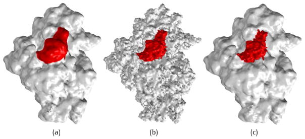
Surface construction of 1J5E from a two-level summation of Gaussian kernels. (a) Uniformly blurred surface, P_R = 0.05 and P_C = 0.5; (b) all details on the model are strengthened, P_R = 0.5 and P_C = 1.0; and (c) only details on chain B are strengthened, P_R = 0.5 and P_C = 1.0 for chain B while P_R = 0.05 and P_C = 0.5 for the remaining structure.

Fig. 4 shows a macromolecular complex representing the thin filament subunit in muscle fibers. This protein contains 32 peptides, and these chains are grouped into several higher level structures called protein “domains”, including tropomyosin (red) and actin (green). A three-level (residue, chain and domain) summation is utilized here to construct the density map

Fig 4.

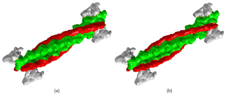
Resolution control of TFC at the domain level, P_R = 0.7, P_C = 0.4. (a) Blurred domain boundary for tropomyosin (red) and actin (green), P_D = 0.25 for the entire protein; and (b) more detailed features are preserved along the boundary of tropomyosin and actin, P_D = 0.8 for these two domains while P_D = 0.25 for the remaining structure.

$$G(\mathbf{x})=\sum _{i_D}{\left(\sum _{i_C}{\left(\sum _{i_R}{\left(\sum _{i_A}{G}_{i_A}(\mathbf{x})\right)}^{P_R}\right)}^{P_C}\right)}^{P_D},$$ (6)

where i_D is the domain index, and P_D is the coefficient corresponding to the domain level. Domain boundaries are blurred with a small coefficient P_D, resulting in a smooth biomolecular surface (Fig. 4(a)); when P_D is set to be a large value, more detailed features are preserved along the domain boundaries (Fig. 4(b)). Although P_D controls the transition region between different domains, the surface resolution inside each domain is mainly decided by the lower level coefficients P_C and P_R. To have a full control of the multi-scale biomolecular models, the number of levels in the summation of Gaussian kernel functions should be consistent with the level of biomolecular structures.

Discussion

In a two-level summation, there are two coefficients: P_C and P_R. P_C controls the boundary resolution of each chain, and P_R controls the surface resolution inside the chain. In a three-level summation, there is one more coefficient (P_D), which controls the boundary resolution of each domain. This local resolution control is very important in some applications such as the diffusional distribution simulation of the calcium ions in ventricular myocytes. Usually, the active site is a small region around certain residues. To simplify the implicit model, we can use a small P_D value to blur the domain boundary, and adjust the P_C and P_R values to make a smooth surface for the domain while showing more residue-level details at the active sites.

3. Density Map Construction

Computational efficiency is critical in biomolecular modeling, especially for large biomolecular complexes with a complicated structure. When computing the Gaussian density for each grid point, if we consider the contribution from all the atoms in the biomolecule, the time complexity will be O(MN), in which M is the number of atoms and N is the number of grid points. To improve the computational efficiency, the neighboring search algorithm is applied to reduce the number of grid points to be analyzed; and the KD-tree structure and a bounding volume hierarchy (BVH) are used to quickly find the contributing atoms for the Gaussian density at a grid point. Moreover, the multi-core CPU and GPU-assisted parallel computation are also employed to further accelerate the speed.

3.1. Neighboring Search

Biomolecular surface is extracted from the Gaussian density map as an isosurface. The grid cell intersecting with the isosurface is called a boundary cell. Vertices on the biomolecular surface are located either on the edges of (marching cubes [32]) or inside (dual contouring [22]) the boundary cell. Therefore, the biomolecular surface is only determined by the Gaussian density values at the grid points in boundary cells, while an accurate density calculation is not necessary for faraway grids. This property has been used in the accelerated isocontouring method [4], which detects the boundary cells to achieve a fast surface extraction.

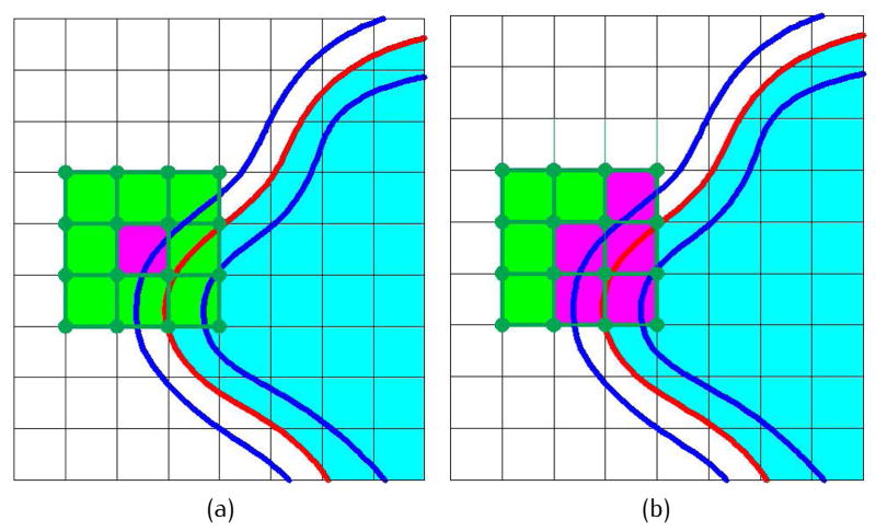
In this paper, a similar idea is adopted and an algorithm called neighboring search [2] is applied to reduce the number of grid points to be analyzed. This algorithm can find out all the grid points near the expected isosurface, as long as the biomolecular surface is a manifold. Therefore, we only need to calculate the Gaussian density at these grid points, while the density value for the other grids is simply set as a constant. k_A is the ratio of the analyzed grid points over the total grid points. k_A is controlled by a pair of predefined parameters: a lower threshold d_l and an upper threshold d_u. Fig. 5 shows an example of neighboring search. The blue curves represent the isosurfaces of d_l and d_u. The red curve represents the target surface. The green cells are the 1-ring neighbors of a given activated grid cell (magenta). The initially activated cell can be found by searching along a line passing through the center of the grid. For each neighboring cell, the Gaussian density values are computed at the eight vertices. If the density indicates that the cell intersects with the band between the blue curves, the cell is activated. More cells can be activated around the newly activated cells iteratively until there are no more updates. As a result, all the grid points close to the surface are analyzed, while faraway points are ignored. Using a flood fill algorithm, those faraway points are marked as interior or exterior grids. Fig. 6 shows the neighboring search results for 2KFX. In (a), the green region represents the inside volume; and in (b) and (c), the green regions represent the band between d_l and d_u. k_A varies with different d_l and d_u, and also depends on the resolution of the grids. It is generally a very small value, see Table 1.

Fig 5.

The neighboring search algorithm. (a) The activated grid cell (magenta) and its 1-ring neighbors; and (b) the newly activated cell (magenta) in the 1-ring neighbors.

Fig 6.

Neighboring search results for 2KFX. (a) The interior domain (green); (b) one detected band using d_l = 0.9, d_u = 1.1 and k_A = 0.026; and (c) another detected band using d_l = 0.1, d_u = 2.0 and k_A = 0.12.

Table 1.

Ratio of analyzed grid points in 2KFX (513 × 513 × 513).

Lower threshold dl	Upper threshold du	Analyzed ratio kA
0.9	1.1	0.026
0.6	1.4	0.048
0.3	1.7	0.092
0.1	2.0	0.12

Discussion

Neighboring search can effectively improve the complexity of Gaussian density computation from O(MN) to O(k_AMN), in which k_A is output-dependent. This method is based on the assumption that the biomolecular surface is a manifold and all the grid points close to the expected surface are neighboring to each other. But sometimes biomolecules have isolated components. If any isolated component is missed in the initial search, the modeling result would be incorrect. However, if the biomolecular structure is known beforehand, the initial search route can be easily modified to include all the components.

3.2. KD-tree Structure and Bounding Volume Hierarchy

A Gaussian kernel function decays quickly as it moves away from the atom center. For one grid point, it is reasonable to ignore faraway atoms, which contribute little to the Gaussian density map. Two methods are used here to quickly find the nearby atoms: the KD-tree structure and the bounding volume hierarchy (BVH).

The KD-tree structure is a widely used space-partitioning data structure, which has been employed in biomolecular modeling [24, 25, 39]. Differently, in this paper a KD-tree is used to quickly search atoms around grid points. The cost to build this data structure is O(M log M). Searching atoms within a certain range around a grid point becomes quite efficient due to the binary tree structure. The error of ignoring faraway atoms can be controlled by a bounding radius R_kd in the KD-tree search. Suppose an atom is ignored when its density contribution is less than ε, then R_kd should satisfy $e^{\kappa (R_{kd}^2-r^2)}<\epsilon$. We have

$$R_{kd}>\sqrt{\frac{\text{ln}\epsilon }{\kappa }+r^2},$$ (7)

where r is the radius of the atom; and κ is the decay ratio in Eqn. 1. Pratically, the maximum atom radius is usually 2.0 Å and the decay ratio is 1.0. When ε = 10⁻⁶, the bounding radius R_kd = 4.3 ensures that no atom around a grid point has a density contribution smaller than ε. For each analyzed grid point, it takes O(log M) to find the nearby atoms and compute the Gaussian density.

The bounding volume hierarchy is a tree structure on a set of geometric objects. All geometric objects are wrapped in bounding volumes that form the leaf nodes of the tree. This technique has been widely used in computer visulization, and also employed in protein structure representation [14, 33, 39]. In this paper, edges of the bounding volumes are along the coordinate axes. The smallest box that contains all the atom centers belonging to a structure is called the minimum bounding box of this structure. The minimum bounding box is generally expanded by a certain ratio. The margin of the bounding box is constraint with at least R_BVH = 4.3 to make sure all the contributing atoms can be searched (similar with Eqn. 7). The bounding box of a higher level structure contains bounding boxes of lower structures. Fig. 7 shows an example of the BVH for a protein with an atom-residue-chain structure. In Fig. 7(a), the space is subdivided into the bounding boxes (red and green) of two peptides. The bounding boxes of peptides are further subdivided into the bounding boxes of residues (Fig. 7(b)). The subdivision allows overlaps and gaps between the children boxes. Searching nearby atoms follows a top-down order in the BVH tree structure. The time complexity for the BVH searching can be O(log M), but in practice the efficiency would be a bit worse because the structures usually have many overlaps. Moreover, as the atom order is organized following the hierarchical structure, the construction of the BVH tree can be easily conducted.

Fig 7.

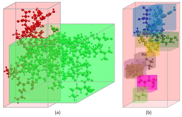
The bounding box system. (a) The bounding boxes of two peptides; and (b) the bounding box of one peptide is subdivided into bounding boxes of residues.

3.3. Parallel Gaussian Density Computation

To further accelerate the speed, multi-core CPU and GPU-based parallel computation are applied in the Gaussian density calculation. In each step of the neighboring search, the grid points to be analyzed are distributed to different threads, and the returned Gaussian density value is used as the input of the next step. The workload for various grid points can be very different because the number of contributing atoms can vary a lot. For the 8-core CPU mode, the grid points are randomly distributed to different cores and the computation keeps at full load for most of the time. Differently, the workload imbalance can seriously influence the performance of the GPU-based computation. Therefore for GPU computation, the contributing atom number of the previously analyzed grids are recorded, and the workload of the newly analyzed grid points is estimated using these numbers. Grid points with similar estimated workload are distributed to the same GPU blocks to achieve a better balance.

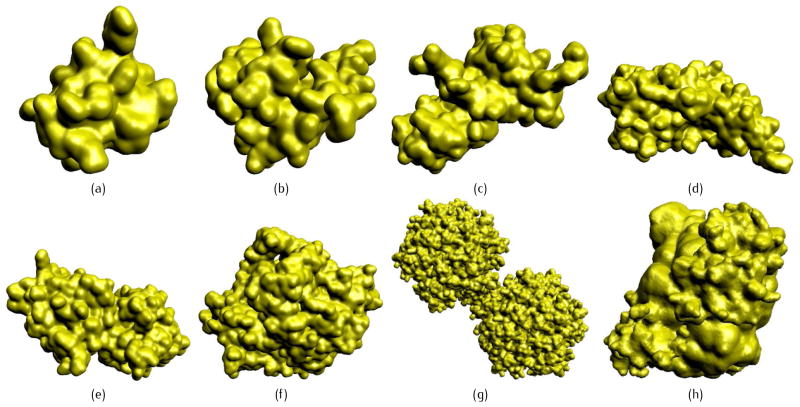
As shown in Fig. 8, a variety of proteins are tested using neighboring search, the KD-tree structure and the BVH. A 2-level summation of Gaussian kernel functions are used, with P_R = 0.5 and P_C = 1.0. Time costs are listed in Table 2. The rectilinear grid for each protein is large enough to contain all the atom centers inside, and the margin on each dimension is 4.0 Å. For all the proteins, we fix the resolution of the grid to be 0.25 Å. The CPU-based results in Table 2 are obtained under 8-core parallel computation. All the results are generated with an Intel E5-1620 CPU, a Nvidia GeForce GTX680 graphic card and 16GB memory. The algorithms are implemented in C++ by using OpenMP for the multi-core CPU computation and CUDA 5.0 for the GPU computation. T₀ is the time cost of CPU computation without any acceleration algorithms. Neighboring search, KD-tree structure and BVH are compared in CPU-based implementations.

Fig 8.

Eight proteins tested in Table 2. (a) 1BOR; (b) 1NEQ; (c) 1A63; (d) 1A7M; (e) 1BEB; (f) 1VNG; (g) 1GTP; and (h) 2KXH.

Table 2.

Efficiency comparison for neighboring search, the KD-tree and BVH. (Grid resolution: 0.25 Å; Unit: second)

PDB ID	M	N	T0	TCPU(NS)	TCPU(KD)	TCPU(BVH)	TCPU(NS+KD)	TGPU(NS+BVH)
1BOR	832	147× 149× 154	3.89	0.76(×5.14)	1.81(×2.15)	2.08(×1.87)	0.65(×6.01)	0.20(×19.44)
1NEQ	1,187	196× 179× 175	8.83	1.08 (×8.21)	2.48(×3.55)	2.73(×3.23)	0.93 (×9.53)	0.25(×35.33)
1A63	2,065	275× 176× 183	21.60	2.56(×8.45)	5.61(×3.85)	6.57(×3.29)	1.50 (×14.40)	0.33(×65.45)
1A7M	2,809	188× 260× 218	34.93	3.37(×10.36)	8.91(×3.92)	9.87(×3.54)	2.03(×17.23)	0.51(×68.49)
1BEB	4,972	232× 246× 324	107.38	8.85(×12.13)	18.77(×5.72)	20.65(×5.20)	2.99(×35.94)	0.92(×116.71)
1VNG	8,808	319× 258× 307	262.19	20.36(×12.88)	36.42(×7.20)	35.43(×7.40)	6.19(×42.37)	1.20(×218.49)
1GTP	69,980	915× 591× 345	15,496.44	820.79(×18.88)	2,060.70(×7.52)	501.83(×30.88)	162.01(× 95.65)	11.33(×1,367.74)
2KXH	70,200	281× 284× 256	2,307.54	159.50(×14.47)	253.02(×9.12)	288.08(×8.01)	20.69(×111.54)	2.71(×851.49)

Note: M - the atom number; N - the grid size; T₀ - CPU computation without any acceleration algorithm; NS - neighboring search; KD - KD-tree structure; BVH - bounding volume hierarchy. The numbers in parentheses are the speedups compared to T₀.

Generally, as the atom number M increases, the speedups for neighboring search, KD-tree and BVH all become more significant. For KD-tree and BVH, the time complexity of Gaussian density map generation is improved to O(N log M), compared with the original O(NM). Therefore, it is easy to understand that the speedups of KD-tree and BVH increase as M gets larger. For neighboring search, the corresponding time complexity is O(k_ANM). At a certain resolution, k_A decreases as M gets larger because generally the surface area grows much slower than the grid size increases. Therefore, the speedup of neighboring search also increases as M gets larger. Besides atom number, the efficiency speedups are also affected by the biomolecular structure. The performance of BVH is directly related to the hierarchical structure of the biomolecules, while the KD-tree is not. For example, 1GTP and 2KXH have similar atom numbers, but the structures in 2KXH are much tighter than in 1GTP, leading to many more overlaps among the bounding boxes. Therefore, the speedup of BVH for 2KXH (8.01 times) is not as significant as 1GTP (30.88 times).

T_CPU(NS+KD) and T_GPU(NS+BVH) shows the effect of different combinations of the techniques. As the hierarchical structure information is ignored in the KD-tree, a re-organization of the atoms is required for multi-level summation of Gaussian kernel functions. The re-organization needs a lot of memory. Therefore instead of KD-tree, the BVH is chosen for GPU-based computation. The combination of neighboring search, KD-tree structure and multi-core CPU computation results in a speedup varying from 6.01 to 111.54 times. For the combination of neighboring search, BVH and GPU computation, the speedup can range from 19.44 times for the smallest protein (1BOR) to 1,367.74 times for the largest protein (1GTP), due to the highly parallel computational capability of the GPU and the maximum effect of neighboring search.

4. Mesh Generation

The dual contouring method [22, 50] is applied to generate adaptive tetrahedral meshes from the Gaussian density map. The multi-core CPU and GPU-based parallel computation are employed to speed up mesh generation.

4.1. Dual Contouring Method

The biomolecular surface is defined as an isosurface of the Gaussian density map, from which tetrahedral meshes can be extracted using the dual contouring method [50, 52]. A strongly-balanced octree structure is built from the rectilinear grid that contains the Gaussian density, and the mesh adaptation is controlled by a feature sensitive error function [50]. To resolve topology ambiguities, we detect ambiguious cells using a trilinear function, and then split them into tetrahedral cells [51]. For each octree cell, the minimum and maximum (min-max) density values are calculated, making it easy to tell if the octree cell is inside or outside the domain to be meshed. For each leaf cell, a dual vertex is generated and the tetrahedral mesh is constructed by connecting the dual vertices with octree grids. For each octree boundary cell that intersects with the biomolecular surface, we choose the mass center as the dual vertex. The mass center is defined as the the average of all the intersection points between the biomolecular surface and the cell edges. For interior leaf cells, the dual vertex is the cell center.

Tetrahedral elements are generated around each minimal edge, which is defined as an edge of a leaf cube that do not properly contain any edge of its neighbors. The minimal edge intersecting with the biomolecular surface is called a sign change edge, and those inside the domain to be meshed are called interior edges. For each sign change edge, we first find out all its surrounding leaf cells and obtain three or four dual vertices. These dual vertices and the interior grid point of this edge form a tetrahedron or a pyramid. For each interior edge, we also obtain three or four dual vertices. Differently, these dual vertices and two endpoints of this edge form a pyramid or a diamond. Later, the pyramids and diamonds can be splitted into tetrahedra. The ambiguous leaf cells are split into tetrahedra, and meshes are generated by analyzing the edges of these tetrahedra [51].

4.2. Paralleled mesh generation

GPU-based computation has been used in isocontouring for surface mesh generation [38]. Differently, in this paper we aim to apply multi-core CPU and GPU-based techniques to the dual contouring method for adaptive tetrahedral mesh generation. In the twelve edges of one leaf cell, at least three of them are independent. As shown in Fig. 9, we divide all the edges into four groups (orange, green, blue and red), and analyze one group in each step. For example, the orange group (edge e₀₁, e₀₃ and e₀₄) is analyzed for all the leaf cells. Each octree cell is distributed to a CPU or GPU thread, and the connectivity can be constructed in a parallel way. During octree subdivision, the most time-consuming step is the min-max computation, which is more expensive for the lower level octree cells with more grid points. To improve the workload balance, octree cells at the same or similar levels are distributed to the same GPU blocks.

Fig 9.

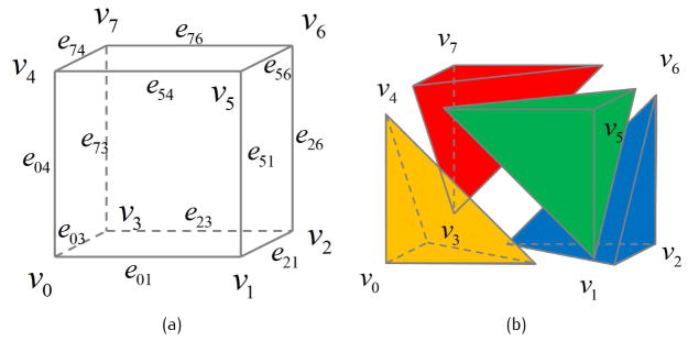
Group of the edges.

5. Quality Improvement

In our generated tetrahedral meshes, most elements are in good quality except some elements around the boundary. Therefore, we need to improve the mesh quality. First, let us choose a few metrics to measure mesh quality [29, 50]: the edge ratio, the Jue-Liu parameter [31], and the dihedral angle. The edge ratio is the ratio of the longest edge length over the shortest edge length in one element. The Joe-Liu parameter is defined as

$$Q=\frac{{8.3}^{\frac{5}{2}}V}{{\left({\sum }_{j=1}^6{e}_j^2\right)}^{\frac{3}{2}}}$$ (8)

where ${\{e_j\}}_{j=1}^6$ are six edge lengths, and V is the volume of a tetrahedron.

Three techniques are applied to improve the mesh quality: face swapping, edge contraction, and geometric flow [29]. Both face swapping and edge contraction are operations of topological optimization. Face swapping reconnects vertices of some elements, while edge contraction removes a few poor quality elements. Differently, geometric flow relocates vertices iteratively to improve the overall mesh quality. Generally speaking, face swapping and edge contraction only change the local topology for a few elements (< 1%), and the process is very fast. Geometric flow smoothing needs to relocate vertices overally, which is the most time-consuming part for quality improvement. Using a similar data structure with [12], the parallel computation is applied to the smoothing step. Vertices are relocated and updated one by one. In the CPU-based computation, METIS [23] is employed to partition the mesh, and vertices in different parts are independent from each other. The location of the vertices on the shared boundaries are synchronized after each smoothing step.

For GPU-assisted computation, vertices are relocated after each step to avoid any conflict. The workload imbalance is the main concern in the implementation. For adaptive meshes, vertices with a large valence number may happen, which can cause serious workload imbalance during the GPU-based geometric flow smoothing. Therefore, vertices are grouped according to their valence number, and the ones with similar valence number are distributed to the same GPU blocks.

6. Results and Discussion

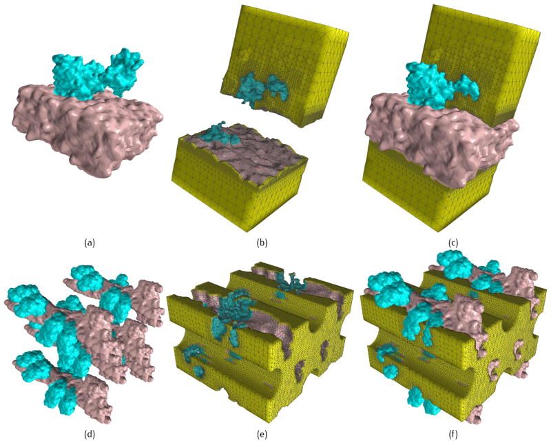
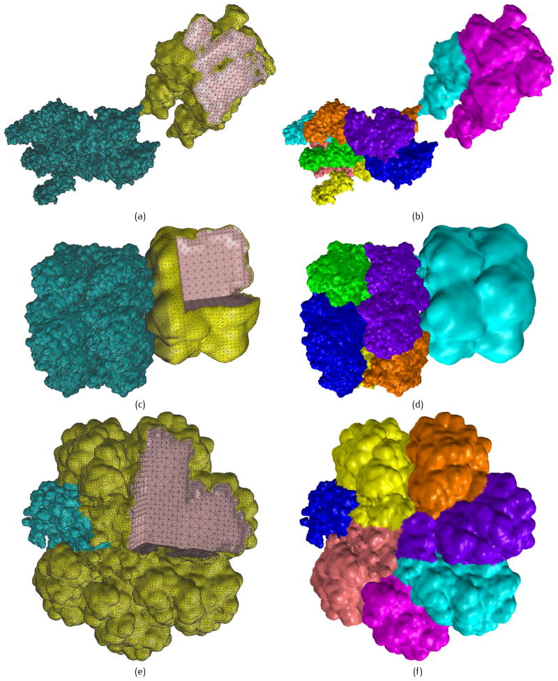
In this section, all the steps in our multi-scale modeling, including Gaussian density computation, mesh generation and quality improvement, are tested in three modes: CPU sequential, CPU 8-core parallel and GPU parallel. Among the tested biomolecular complexes (see Figs. 1, 10 and 11), TFC, the SERCA pump and the myofibril lattice (ML) are from the human cardiac calcium signaling system, while 2W4A, 1HTQ and 2KU2 are chosen from the Protein Data Bank (PDB). A 3-level summation of Gaussian kernel functions is applied for TFC, while the other models use a 2-level summation. Table 3 shows the modeling results, which are generated from a computer with an Intel Xeon E5-1620 CPU, a Nvidia GeForce GTX680 graphic card, and 16GB of memory.

Fig 10.

Two biomolecualr complexes in human cardiac calcium signaling system. (a–c) SERCA pump with P_R = 0.2, P_C = 0.8 and P_R = 0.2, P_C = 1.1 for low and high resolution components, respectively; and (d-f) the myofibril lattice (ML) with P_R = 0.5, P_C = 0.3 and P_R = 0.7, P_C = 0.4 for low and high resolution components, respectively. (a) and (d) show the protein structure with the blue region emphasized in high resolution; (b) and (e) show exterior tetrahedral meshes; and (c) and (f) show exterior meshes with embeded proteins.

Fig 11.

Three large proteins. (a–b) 2W4A with P_R = 0.2, P_C = 0.8 and P_R = 0.4, P_C = 1.2 for low and high resolution components, respectively; (c–d) 1HTQ with P_R = 0.3, P_C = 0.8 and P_R = 1.0, P_C = 1.5 for low and high resolution components, respectively; and (e–f) 2KU2 with P_R = 0.5, P_C = 1.0 and P_R = 1.6, P_C = 2.0 for low and high resolution components, respectively. (a), (c) and (e) show tetrahedral mesh of the proteins with the blue region emphasized in high resolution, and the pink region shows a cross section of the model; (b), (d) and (f) show the partition results in parallel computation.

Table 3.

Time cost for three testing modes (CPU sequential, CPU 8-core parallel and GPU parallel) and mesh statistics. (Unit: second).

Complex	TFC			SERCA			ML			2W4A			1HTQ			2KU2
M	69,222			80,157			95,853			0.19M			0.98M			1.23M
Mode	CS	C-8	G	CS	C-8	G	CS	C-8	G	CS	C-8	G	CS	C-8	G	CS	C-8	G
DM	188.6	37.8 (×5.0)	4.8 (×39.3)	165.1	38.4 (×4.3)	11.7 (×14.1)	377.5	75.6 (×5.2)	7.3 (×51.7)	687.4	143.5 (×4.8)	10.2 (×67.4)	6,494.7	1589.4 (×4.1)	88.4 (×73.5)	3,050.2	645.5 (×4.7)	63.2 (×48.3)
MG	13.2	6.6 (×2.0)	2.4 (×5.5)	12.8	6.3 (×2.0)	2.3 (×5.6)	13.1	6.7 (×2.0)	2.4 (×5.5)	12.9	6.7 (×1.9)	2.4 (×5.4)	13.1	6.7 (×2.0)	2.7 (×4.9)	12.9	6.5 (×2.0)	2.4 (×5.4)
QI	157.8	35.8 (×5.0)	6.3 (×25.2)	163.5	37.7 (×4.3)	7.2 (×22.7)	189.5	36.7 (×5.2)	5.8 (×32.7)	213.7	53.2 (×4.0)	6.5 (×32.9)	250.6	68.3 (×3.7)	12.5 (×20.0)	178.0	44.2 (×4.0)	6.7 (×26.6)
Total	359.6	80.2 (×4.5)	13.5 (×26.6)	341.4	82.4 (×4.1)	21.2 (×16.1)	580.1	119.0 (×4.9)	15.5 (×37.4)	914.0	203.4 (×4.5)	19.1 (×47.9)	6,758.4	1,664.4 (×4.1)	103.6 (×65.2)	3241.1	696.2 (×4.7)	72.3 (×44.8)
Mesh size (V#, E#)	(212,120, 1,094,424)			(190,356, 946,273)			(271,523, 1,327,336)			(276,458, 1,334,008)			(399,994, 1,989,245)			(243,463, 1,201,048)
Edge ratio (min, max)	(1.0, 10.24)			(1.0, 10.23)			(1.0, 10.31)			(1.0, 10.98)			(1.0, 9.56)			(1.0, 10.60)
Joe-Liu (min, max)	(0.12, 1.0)			(0.14, 1.0)			(0.18, 1.0)			(0.11, 1.0)			(0.10, 1.0)			(0.15, 1.0)
Dihedral angle (min, max)	(15.00°, 165.25°)			(15.01°, 167.25°)			(15.03°, 164.20°)			(15.10°, 166.23°)			(15.03°, 167.46°)			(14.86°, 167.42°)

Note: M - atom number; CS - CPU sequential; C-8 - 8-core CPU parallel; G - GPU parallel; DM - time for density map construction; MG - time for mesh generation; QI - time for quality improvement; (V#, E#) - (vertex number, element number).

Thin filament complex (TFC)

The thin filament complex is an important component in myofibrils, which is also the key functional part in the muscle fibers. The contraction of muscle fibers rely heavily on the interaction between the myosin heads and the filaments. To study the calcium ion signaling process during the muscle contraction, a cuboidal outer boundary is inserted around the thin filament, and the exterior tetrahedral meshes are generated, see the 2W4U model in Fig. 1.

SERCA pump

The SERCA pump works as a pump for the calcium ions in the signaling. The system contains a segment of lipid and a protein 1SU4 intersecting with it. As shown in Fig. 10(a–c), a cuboidal boundary is insert around it and intersecting with the membrane. The exterior mesh is generated which is divided by the membrane into two separated parts.

Myofibril lattice (ML)

During the heart muscle contraction, the calcium signaling process is a combination of the interaction between the thin and thick filaments. A model containing six thin filaments and four thick filaments is built with a cuboidal outer boundary intersecting with the filaments, see Fig. 10(d–f). The exterior tetrahedral mesh is generated to represent the environment around the filaments. The thin filaments here contains six myosin heads, and the thick filaments are represented by cylinders. The density map for a single thin filament is generated using the multi-level summation of Gaussian kernel functions, it is used for the assembly of the intact density map containing six thin filaments. The assembly step costs about ten seconds, which is not count in Table 3.

As shown in Fig. 11, three large proteins are chosen from the Protein Data Bank, and tested using our modeling methods. 2W4A is a contractile protein for insect flight muscle. 1HTQ is a glutamine synthetase from Mycobacterium tuberculosis, the second largest protein we found in the PDB. 2KU2 is a hydrolase protein, which is also the largest protein we found in the PDB.

In Gaussian density map generation, the rectilinear grid size for the Gaussian density map is constraint to be 513 × 513 × 513. For the CPU-based computation, neighboring search and the KD-tree structure are applied in both the sequential and parallel modes; while the combination of neighboring search and BVH is employed in the GPU-based mode. The speedups of the 8-core CPU computation are similar for all the complexes (4.1~5.2), while the speedups of the GPU-assisted computation vary from 14.1 to 73.5 times. The worst speedup of the GPU computation happens on the SERCA pump, as shown in Fig. 10(a). In SERCA pump, the lipid (pink) contains most of the atoms without a hierarchical structure, which greatly reduces the subdivision efficiency of the BVH.

In both 8-core CPU and GPU-based computation, the time costs of mesh generation are similar for all the tested models although the mesh size differs. This is because in mesh generation, the most time-consuming step is octree subdivision. Compared to the uniform grids, the adaptive octree construction requires a much more complicated index system, which significantly limits the speedups. From Table 3, we can observe that the speedups are 1.9~2.0 times for the 8-core CPU computation, and 4.9~5.6 times for the GPU-based computation.

During quality improvement, for both the CPU sequential and the 8-core CPU computation, we can observe that the time cost increases as the mesh size becomes larger. However, it is more complicated for the GPU-based computation due to its high sensitivity to the vertex valence number, which also brings in serious workload imbalance on different threads. As discussed in Section 5, high valence numbers are introduced by mesh adaptation. In particular, TFC, the SERCA pump, and 1HTQ contain large volumes, and they require more adaptive meshes to reduce the mesh size. Due to this reason, a workload imbalance is introduced in their GPU computation. Therefore, for these three models the speedups are only about 20.0~25.2 times, not as significant as the others (26.6~32.9 times).

For the whole modeling process, the 8-core CPU computation introduces a similar speedup on the efficiency for all the tested proteins (4.1~4.9 times), while the speedups of the GPU-assisted computation vary from 16.1 to 65.2 times. In addition, from Table 3 we can observe that the obtained meshes are in good quality with the minimal dihedral angle ≥ 14.86°.

7. Conclusion and Future Work

In this paper, a multi-level summation of Gaussian kernel functions is applied to generate multi-scale implicit models for the biomolecules. Structures at different levels are specified and emphasized with more details on the local surface. The computational efficiency is improved by using a combination of neighboring search, KD-tree structure and bounding volume hierarchy. The CPU and GPU-assisted parallel computation techniques are employed in all the modeling steps, including Gaussian density map construction, mesh generation and quality improvement. In our approach, large proteins can be modeled quickly with quality adaptive tetrahedral meshes as output.

In the future, it is worth to apply the multi-level summation of Gaussian kernel functions in various application problems such as the diffusion simulation and boundary element solvers of the Poisson-Boltzmann equation [15, 16, 34]. In particular, the study of large biomolecules will benefit a lot from the high efficiency introduced by our techniques. The multi-level summation can also be extended to work for a combination of biomolecular information from the Protein Data Bank and Cryo-EM scanned images.

References

- 1.Albou L, Schwarz B, Poch O, Wurtz J, Moras D. Defining and characterizing protein surface using alpha shapes. Proteins. 2009;76(1):1–12. doi: 10.1002/prot.22301. [DOI] [PubMed] [Google Scholar]
- 2.Artemova S, Grudinin S, Redon S. A comparison of neighbor search algorithms for large rigid molecules. Journal of Computational Chemistry. 2011;32(13):2865–2877. doi: 10.1002/jcc.21868. [DOI] [PubMed] [Google Scholar]
- 3.Bajaj CL, Castrillon-Candas J, Siddavanahalli V, Xu Z. Compressed representations of macromolecular structures and properties. Structure. 2005;13:463–471. doi: 10.1016/j.str.2005.02.004. [DOI] [PubMed] [Google Scholar]
- 4.Bajaj CL, Pascucci V, Schikore D. Technical report. Texas Institute of Computational and Applied Mathematics; 1999. Seed sets and search structures for optimal isocontour extraction. [Google Scholar]
- 5.Bajaj CL, Pascucci V, Shamir A, Holt RJ, Netravali AN. Technical report, TICAM Technical Report. 1999. Multiresolution molecular shapes. [Google Scholar]
- 6.Bajaj CL, Pascucci V, Shamir A, Holt RJ, Netravali AN. Dynamic maintenance and visualization of molecular surfaces. Discrete Applied Mathematics. 2003;127(1):23–51. [Google Scholar]
- 7.Bajaj CL, Siddavanahalli V. Technical report, ICES 06-03. 2006. Fast error-bounded surfaces and derivatives computation for volumetric particle data. [Google Scholar]
- 8.Blinn JF. A generalization of algebraic surface drawing. ACM Transactions on Graphics. 1982;1(3):235–256. [Google Scholar]
- 9.Cheng Y, Chang CA, Yu Z, Zhang Y, Sun M, Leyh TS, Holst MJ, Mccammon JA. Diffusional channeling in the sulfate activating complex: combined continuum modeling and coarsegrained Brownian dynamics studies. Biophysical Journal. 2008;95(10):4659–4667. doi: 10.1529/biophysj.108.140038. [DOI] [PMC free article] [PubMed] [Google Scholar]
- 10.Connolly ML. Analytical molecular surface calculation. Journal of Applied Crystallography. 1983;16(5):548–558. [Google Scholar]
- 11.Connolly ML. Network Science. 1996. Molecular surface: A Review. [Google Scholar]
- 12.D’Amato JP, Vénere M. A CPU-GPU framework for optimizing the quality of large meshes. Journal of Parallel and Distributed Computing. 2013 (0):–. [Google Scholar]
- 13.Edelsbrunner H, Mücke EP. Three-dimensional alpha shapes. ACM Transactions on Graphics. 1994;13(1):43–72. [Google Scholar]
- 14.Fonseca R, Winter P. Bounding volumes for proteins: a comparative study. Journal of Computational Biology. 2012;19(10):1203– 1213. doi: 10.1089/cmb.2012.0104. [DOI] [PubMed] [Google Scholar]
- 15.Geng W, Jacob F. A GPU-accelerated direct-sum boundary integral Poisson-Boltzmann solver. Computer Physics Communications. 2013;184:1490–1496. [Google Scholar]
- 16.Geng W, Krasny R. A treecode-accelerated boundary integral Poisson-Boltzmann solver for electrostatics of solvated biomolecules. Journal of Computational Physics. 2013;247:62–87. [Google Scholar]
- 17.Geng W, Zhao S. Fully implicit ADI schemes for solving the nonlinear Poisson-Boltzmann equation. Molecular Based Mathematical Biology. 2013;1:109–123. [Google Scholar]
- 18.Giard J, Macq B. Molecular surface mesh generation by filtering electron density map. International Journal of Biomedical Imaging. 2010:263–269. doi: 10.1155/2010/923780. [DOI] [PMC free article] [PubMed] [Google Scholar]
- 19.Grant JA, Pickup BT. A Gaussian description of molecular shape. Journal of Physical Chemistry. 1995;99(11):3503–3510. [Google Scholar]
- 20.Holst M, Baker N, Wang F. Adaptive multilevel finite element solution of the Poisson-Boltzmann equation algorithms I: algorithms and examples. Journal of Computational Chemistry. 2000;21:1319–1342. [Google Scholar]
- 21.Hu L, Chen D, Wei G. High-order fractional partial differential equation transform for molecular surface construction. Molecular Based Mathematical Biology. 2013;1:1–25. doi: 10.2478/mlbmb-2012-0001. [DOI] [PMC free article] [PubMed] [Google Scholar]
- 22.Ju T, Losasso F, Schaefer S, Warren J. Dual contouring of Hermite data. SIGGRAPH. 2002;21:339–346. [Google Scholar]
- 23.Karypis G, Kumar V. A fast and high quality multilevel scheme for partitioning irregular graphs. SIAM J Sci Comput. 1998;20(1):359–392. [Google Scholar]
- 24.Kim B, Kim KJ, Seong JK. GPU accelerated molecular surface computing. Appl Math. 2012;6(1S):185S–194S. [Google Scholar]
- 25.Kim DS, Kim JK, Cho Y, Kim CM. Querying simplexes in quasi-triangulation. Computer-Aided Design. 2012;44(2):85– 98. [Google Scholar]
- 26.Kim DS, Seo J, Kim D, Ryu J, Cho CH. Three-dimensional beta shapes. Computer-Aided Design. 2006;38(11):1179–1191. [Google Scholar]
- 27.Laug P, Borouchaki H. Molecular surface modeling and meshing. Engineering with Computers. 2002;18:199–210. [Google Scholar]
- 28.Lee MS, Feig M, Salsbury FR, Brooks CL. New analytic approximation to the standard molecular volume definition and its application to generalized born calculations. Journal of Computational Chemistry. 2003;24(14):1348–1356. doi: 10.1002/jcc.10272. [DOI] [PubMed] [Google Scholar]
- 29.Leng J, Zhang Y, Xu G. A novel geometric flow-driven approach for quality improvement of segmented tetrahedral meshes. Proceedings of the 20th International Meshing Roundtable; 2012. pp. 347–364. [Google Scholar]
- 30.Li W, McMains S. Voxelized Minkowski sum computation on the GPU with robust culling. Computer-Aided Design. 2011;43(10):1270– 1283. [Google Scholar]
- 31.Liu A, Joe B. Relationship between tetrahedron shape measures. BIT Numerical Mathematics. 1994;34:268–287. [Google Scholar]
- 32.Lorensen WE, Cline HE. Marching cubes: a high resolution 3D surface construction algorithm. SIGGRAPH. 1987;21(4):163–169. [Google Scholar]
- 33.Lotan I, Schwarzer F, Halperin D, Latombe J. Algorithm and data structures for efficient energy maintenance during Monte Carlo simulation of proteins. Journal of Computational Biology. 2004;11(5):902– 932. doi: 10.1089/cmb.2004.11.902. [DOI] [PubMed] [Google Scholar]
- 34.Lu B, Cheng X, McCammon JA. “New-version-fast-multipole-method” accelerated electrostatic interactions in biomolecular systems. Journal of Computational Physics. 2007;226:1348–1366. doi: 10.1016/j.jcp.2007.05.026. [DOI] [PMC free article] [PubMed] [Google Scholar]
- 35.Pavanaskar S, McMains S. Filling trim cracks on GPU-rendered solid models. Computer-Aided Design. 2013;45(2):535– 539. [Google Scholar]
- 36.Ryu J, Park R, Kim DS. Molecular surfaces on proteins via beta shapes. Computer-Aided Design. 2007;39(12):1042–1057. [Google Scholar]
- 37.Sanner MF, Olson AJ, Spehner JC. Reduced surface: an efficient way to compute molecular surfaces. Biopolymers. 1996;38(3):305–20. doi: 10.1002/(SICI)1097-0282(199603)38:3%3C305::AID-BIP4%3E3.0.CO;2-Y. [DOI] [PubMed] [Google Scholar]
- 38.Schmitz L, Scheidegger LF, Osmari DK, Dietrich CA, Comba JLD. Efficient and quality contouring algorithms on the GPU. Computer Graphics Forum. 2010;29:2569– 2578. [Google Scholar]
- 39.Seong JK, Baek N, Kim KJ. Real-time approximation of molecular interaction interfaces based on hierarchical space decomposition. Computer-Aided Design. 2011;43(12):1598– 1605. [Google Scholar]
- 40.Song Y, Zhang Y, Bajaj CL, Baker NA. Continuum diffusion reaction rate calculations of wild-type and mutant mouse acetylcholinesterase: adaptive finite element analysis. Biophysical Journal. 2004;87(3):1558–1566. doi: 10.1529/biophysj.104.041517. [DOI] [PMC free article] [PubMed] [Google Scholar]
- 41.Song Y, Zhang Y, Shen T, Bajaj CL, McCammon JA, Baker NA. Finite element solution of the steady-state Smoluchowksi equation for rate constant calculations. Biophysical Journal. 2004;86(4):2017–2029. doi: 10.1016/S0006-3495(04)74263-0. [DOI] [PMC free article] [PubMed] [Google Scholar]
- 42.Stone JE, Hardy DJ, Ufimtsev IS, Schulten K. GPU-accelerated molecular modeling coming of age. Journal of Molecular Graphics and Modelling. 2010;29(2):116– 125. doi: 10.1016/j.jmgm.2010.06.010. [DOI] [PMC free article] [PubMed] [Google Scholar]
- 43.Varshney A, Brooks FP., Jr Fast analytical computation of richards’s smooth molecular surface. Proceedings of the IEEE Visualization; 1993. pp. 300–307. [Google Scholar]
- 44.Wang CL, Manocha D. GPU-based offset surface computation using point samples. Computer-Aided Design. 2013;45(2):321– 330. [Google Scholar]
- 45.Wang Q, JaJa J, Varshney A. An efficient and scalable parallel algorithm for out-of-core isosurface extraction and rendering. Journal of Parallel and Distributed Computing. 2007;67(5):592–603. [Google Scholar]
- 46.Wei G, Sun Y, Zhou Y, Feig M. Molecular multiresolution surfaces. arXiv math-ph/0511001. 2005 [Google Scholar]
- 47.Xie Y, Cheng J, Lu B, Zhang L. Parallel adaptive finite element algorithms for solving the coupled electro-diffusion equations. Molecular Based Mathematical Biology. 2013;1:90–108. [Google Scholar]
- 48.Yu Z, Holst Michael J, Cheng Y, McCammon JA. Feature-preserving adaptive mesh generation for molecular shape modeling and simulation. Journal of Molecular Graphics and Modeling. 2008;26(8):1370–1380. doi: 10.1016/j.jmgm.2008.01.007. [DOI] [PubMed] [Google Scholar]
- 49.Zhang D, Suen J, Zhang Y, Song Y, Radic Z, Taylor P, Holst MJ, Bajaj CL, Baker NA, Mc-Cammon JA. Tetrameric mouse acetylcholinesterase: continuum diffusion rate calculations by solving the steady-state Smoluchowski equation using finite element methods. Biophysical Journal. 2005;88(3):1659–1665. doi: 10.1529/biophysj.104.053850. [DOI] [PMC free article] [PubMed] [Google Scholar]
- 50.Zhang Y, Bajaj CL, Sohn B. 3D finite element meshing from imaging data. Computer Methods in Applied Mechanics and Engineering. 2005;194(48—49):5083–5106. doi: 10.1016/j.cma.2004.11.026. [DOI] [PMC free article] [PubMed] [Google Scholar]
- 51.Zhang Y, Qian J. Resolving topology ambiguity for multiple-material domains. Computer Methods in Applied Mechanics and Engineering. 2012;247–248:166–178. [Google Scholar]
- 52.Zhang Y, Xu G, Bajaj CL. Quality meshing of implicit solvation models of biomolecular structures. Computer Aided Geometric Design. 2006;23(6):510–530. doi: 10.1016/j.cagd.2006.01.008. [DOI] [PMC free article] [PubMed] [Google Scholar]
- 53.Zheng Q, Yang S, Wei G. Biomolecular surface construction by PDE transform. International Journal for Numerical Methods in Biomedical Engineering. 2012;28(3):291–316. doi: 10.1002/cnm.1469. [DOI] [PMC free article] [PubMed] [Google Scholar]