Metabolite Profiling of Plastidial Deoxyxylulose-5-Phosphate Pathway Intermediates by Liquid Chromatography and Mass Spectrometry

Abstract

Metabolite profiling is a powerful tool that enhances our understanding of complex regulatory processes and extends to the comparative analysis of plant gene function. However, at present, there are relatively few examples of metabolite profiling being used to characterize the regulatory aspects of the plastidial deoxyxylulose-5-phosphate (DXP) pathway in plants. Since the DXP pathway is one of two pathways in plants that are essential for isoprenoid biosynthesis, it is imperative that robust analytical methods be employed for the characterization of this metabolic pathway. Recently, liquid chromatography-mass spectrometry (LC-MS), in conjunction with traditional molecular biology approaches, established that the DXP pathway metabolite, methylerythritol cyclodiphosphate (MEcPP), previously known solely as an intermediate in the isoprenoid biosynthetic pathway, is a stress sensor that communicates environmental perturbations sensed by plastids to the nucleus, a process referred to as retrograde signaling. In this chapter, we describe two LC-MS methods from this study that can be broadly used to characterize DXP pathway intermediates.

1 Introduction

The DXP pathway, also known as the methylerythritol 4-phosphate (MEP) pathway, consists of seven enzymes that transform glyceraldehdye-3-phosphate (G3P) and pyruvic acid to intermediates and the final products namely, isopentenol diphosphate (IPP) and dimethylallyl diphosphate (DMAPP) (Fig. 1), from which all isoprenoids are synthesized [1–4]. DXP pathway intermediates can be anionic in nature and, therefore, carry net negative charges. This means that they are detected as deprotonated ions [M–H]⁻ in the negative mode of mass spectrometry. However, when profiling metabolites, it is better to separate them in real-time prior to their detection. The addition of this separation step reduces ion suppression effects (in electrospray ionization, ESI) caused from interfering compounds and, thus, improves upon quantitation.

Fig. 1.

Overview of the DXP pathway. Intermediates of the DXP pathway are as follows: Pyruvate (pyr) and glyceraldehyde 3-phosphate (G3P) are condensed to DXP with a loss of carbon dioxide, a reaction performed by DXP synthase (DXS); DXP is reduced to methylerythritol phosphate (MEP) by DXP reductoisomerase (DXR); MEP reacts with cytidine triphosphate to produce diphosphocytidylyl methylerythritol (CDP-ME), a reaction catalyzed by MEP cytidylyltransferase (MCT); CDP-ME is phosphorylated to CDP-ME phosphate (CDP-MEP) by CDP-ME kinase (CMK); CDP-MEP is converted to MEcPP via a loss of cytidine monophosphate, a reaction catalyzed by MEcPP synthase (MDS); MEcPP is converted to hydroxymethylbutenyl diphosphate (HMBPP) by HMBPP synthase (HDS); HMBPP is converted to IPP and DMAPP by HMBPP reductase (HDR); IPP can be reversibly isomerized to DMAPP via IPP isomerase (IDI). MEcPP is thought to undergo reduction and elimination to HMBPP [4]

Separation of hydrophilic compounds such as the intermediates of the DXP pathway is generally best achieved by ion exchange chromatography (IXC), ion exclusion chromatography (IEC), and hydrophilic interaction liquid chromatography (HILIC). In IXC, retention is based on the interaction between the charged analyte and the charged functional groups bound to the stationary phase [5, 6]. This retention property enables anionic metabolites, such as the DXP pathway intermediates, to be retained by their interaction with the positively charged groups on the stationary phase. In IEC, ions with the same charge as the stationary phase (such as those from the mobile phase) are not permitted to penetrate it as they are excluded through repulsion [5, 6]. Here, only the analyte is allowed to interact with the stationary phase. A stationary phase that employs both mechanisms is normally composed of a resin. The charged groups on the resin allow for IXC and IEC to take place, and the polystyrene backbone of the resin allows for hydrophobic interactions. The resin, therefore, permits the retention mechanisms of reversed phase, normal phase partitioning, and size exclusion to occur. These multiple modes of interaction provide resin-based HPLC columns with added selectivity under isocratic conditions [5, 6]. However, a major drawback to using this approach with mass spectrometry (MS) is that analyte separation is normally achieved via aqueous mobile phases.

HILIC retention is achieved through hydrogen bonding between the analyte and water bound to the silica stationary phase [7]. Consequently, analytes are best retained by the stationary phase when the organic content (e.g., acetonitrile) of the mobile phase is high and they are eluted from the column when the aqueous content of the mobile phase is high. Secondary interactions can be achieved through the addition of charged groups (e.g., zwitter ions) to the silica stationary phase to further improve upon the selectivity of the HILIC method [8]. The volatile nature of HILIC mobile phases makes this separation technique ideally suited to electrospray mass spectrometry (ESI-MS).

Once the separated metabolites have been eluted from the column they are delivered to the ion source. Here, they are converted to gaseous ions by the combination of a nebulizer gas and a heated drying gas during ESI. This ionization technique is established via the application of a strong electric field, under atmospheric pressure, to the eluent passing through a narrow stainless steel capillary, where the accumulation of charge at the liquid surface at the tip of the capillary leads to the formation of highly charged droplets. As the droplets become increasingly smaller the accumulation of destabilizing like-charges, through natural repulsion, causes the release of ions. Consequently a cascade of coulombic repulsions eventually give rise to either an ion contained within a single droplet and/or the emission of solvated ions from charged droplets, which lead to the formation of gas phase ions upon evaporation [9–14].

Ions from the ESI source are electrostatically drawn towards the entrance of the MS, where they pass through a heated sampling capillary until they reach a metal skimmer. From there, they pass through an ion guide (e.g., an octapole) under a specified radio frequency (rf) voltage. The application of a high vacuum at this stage reduces the number of collisions between ions and gas molecules. Before entering the mass analyzer, ions are further focused by a series of lenses [15]. For the purpose of this chapter, only the quadrupole (quad; Fig. 2) and the time-of-flight (TOF; Fig. 3) mass analyzer will be discussed.

Fig. 2.

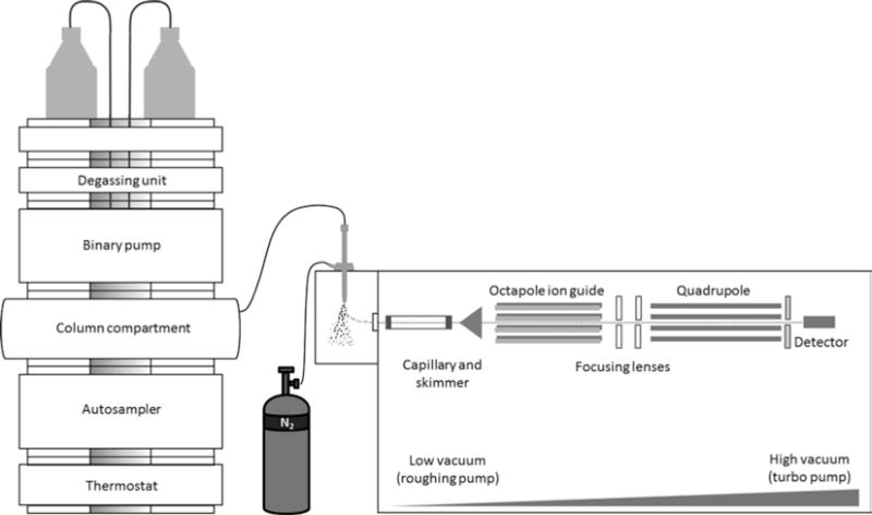
LC-ESI-quad MS. After analyte ions are delivered to the ion source, ESI facilitates their transfer (from the liquid to the gas phase) to the entrance of the MS. From there they are transmitted to the quadrupole (via a glass capillary, a skimmer, and focusing lenses) and transit this mass analyzer in a stable spiral like trajectory at its center (while dc and ac/rf voltages are alternated), en route to the detector. This illustration is based on an Agilent Technologies LC-ESI-quad MS system

Fig. 3.

LC-ESI-TOF MS. After analyte ions are delivered to the ion source, ESI facilitates their transfer (from the liquid to the gas phase) to the entrance of the MS. From there they are transmitted to the TOF (via a glass capillary, a skimmer, an ion guide and focusing lenses) and are pulsed up the flight tube and reflected down (by specific voltages) en route to the detector. Lighter ions arrive at the detector first. This illustration is based on an Agilent Technologies LC-ESI-quad MS system

A single quad is a low resolution, low cost, highly robust mass spectrometer that consists of four parallel cylindrical or hyperbolic rods that are equally spaced around a central axis [16], with each rod serving as an electrode. Opposing sets of rods have both direct current (dc) and radio frequency (rf) voltages applied to them. As ions transit the rods both dc and rf voltages are increased at a constant ratio [17]. The application of these voltages creates an area of mutual stability at the center of the rods, where only ions with certain m/z ratios are transmitted through the quadrupole, whereas ions exhibiting different m/z ratios collide with the rods as result of their unstable trajectories [16]. Thus, the quadrupole forms a low and high mass filter. The relationship of m/z to these potentials is described in following equations:

$$U=a_{\mathrm{u}}=\frac{m}{z}\frac{{\omega }^2{r}_0^2}{8e}V=q_{\mathrm{u}}=\frac{m}{z}\frac{{\omega }^2{r}_0^2}{4e}$$

where a_u and q_u are the stability parameters and e is the charge of an electron [9]. The other parameters ω² and $r_0^2$ are related to the angular frequency and radius, respectively [9]. The output of the dc generator is described by the V voltage and the rf generator is described by the U voltage [9]. To scan a mass spectrum, both voltages are increased at the same time from zero to some maximum value while their ratio is maintained constant [17–19]. A scan is, therefore, achieved in sequential steps, from the lowest to the highest m/z ratio.

In the most sensitive operating mode of the single quadrupole, selected ion monitoring (SIM), the mass analyzer is programmed to allow the passage of ions with specific m/z ratios (typically ±0.5 m/z) through to the detector. In this way, the mass spectrometer spends more time collecting information on preselected ions rather than scanning across a wide mass range. This leads to a reduction in background noise and, by extension, a significant increase in signal-to-noise (see ^{Note 1}). The quad mass analyzer is ideally suited to targeted metabolite analyses, especially when the SIM mode is employed (Fig. 2).

A TOF is a medium to high resolution mass analyzer with an extremely high scan rate (see ^{Note 2}). The TOF mass analyzer consists of a flight tube under a high vacuum. The principle of TOF is based on the assumption that ions with the same initial kinetic energy (E_kin) travel at different velocities ν that are proportional to their m/z ratios and inversely proportional to their masses (m):

$$\mathrm{\nu }=\frac{\sqrt{E_{\mathit{kin}}}}{m}$$

For a given energy (E) and distance (L), the mass is proportional to the square of the flight time (t) [15]:

$$m=t^2\left(\frac{2E}{L^2}\right)$$

The m/z ratio of a given ion can, therefore, be calculated by measuring the time it takes to travel a certain distance [15]:

$$\frac{m}{z}=t^2\left(\frac{2eV}{L^2}\right)\frac{1}{2}$$

where ions are selected by a potential V and e is the charge of an electron [9, 15, 20, 21].

As ions enter the TOF they are subjected to a pulsed electric field, which is applied at the entrance of the TOF. Lighter, multiple-charged ions reach the detector before heavier single-charged ions [15]. Once ions are pulsed up the flight tube, they enter the reflectron region which, as the name suggests, is responsible for repelling ions towards the detector based on their forward kinetic energies (see ^{Notes 3} and ⁴). A consequence of this is that the same ions arrive at the flight tube at the same time (see ^{Note 5}). In this way, the reflectron region improves mass resolution and accuracy by minimizing variations in the flight times of ions (resulting from different spatial and kinetic energy distributions) [15]. The reflectron region also helps to double the flight path, giving ions more time to separate and, hence, increases the overall resolution (the mass difference, Δm, between two adjacent masses) of the mass analyzer (see ^{Note 6}).

The monoisotopic mass is used to determine the mass accuracy of analyte ions, which is the difference between the theoretical m/z ratio and the measured (see ^{Note 7}).

$$\text{Mass accuracy}\left(\mathrm{ppm}\right)=1\times {10}^6\left(\frac{\mathit{mTheo}-\mathit{mMeas}}{\mathit{mTheo}}\right)$$

In the above equation mTheo is the theoretical m/z ratio and mMeas is the measured m/z ratio [22]. The high acquisition rate, high sensitivity, high mass resolution, and high mass accuracy of TOF make this mass analyzer ideally suited to targeted metabolomics analyses (Fig. 3).

Information obtained from MS (i.e., a measure of the characteristics of charged molecules based on the mass-to-charge ratio, m/z, of an ion) is commonly used to deduce elemental composition and elucidate the chemical structure of a compound. A mass spectrometer can, therefore, be used to produce a mass spectrum (a plot of m/z vs. intensity) or used as a detector (a plot of peak intensity vs. time) [6, 16, 17]. An analyte ion is generally quantified by the area under the corresponding chromatographic peak. The TOF utilizes extracted ion chromatograms (EIC) for accurate peak integration, whereas the quad utilizes either EIC (in the full scan mode) or SIM chromatograms, with each data point across the chromatographic peak corresponding to the m/z ratio of the analyte ion (see ^{Note 8}). The added selectivity that the mass spectrometer brings allows LC-MS to be used to quantify metabolites from complex biological matrices such as plant biomass. For a more comprehensive study of IXC, IEC, HILIC, ESI, quad and TOF mass spectrometry, the reader is kindly referred to other sources for this information [5–21]. In this chapter we describe IXC-IEC-ESI-TOF MS and HILIC-ESI-quad MS methods for the measurement of plastidial DXP pathway intermediates.

2 Materials

It is recommended that solvents used for LC-MS experiments are of HPLC grade (99.9 % chemical purity) or greater, and that the chemicals used are of analytical grade (with a chemical purity >90 %). Chemical standard and sample solutions are prepared in acetonitrile–water (1:1, v/v) [1]. Alternatively, they can also be prepared in the appropriate reconstitution medium (i.e., the initial mobile phase solvent composition) (see ^{Note 9}). Filter and degas all HPLC eluents (i.e., with a 0.2- or 0.45-μm membrane pore size filter) prior to use. It is also recommended that a guard column is used as it can prolong the lifetime of the analytical column. Use nitrogen as both the nebulizer and heated drying gas for ESI (see ^{Note 10}). Please remember to follow your institution’s or company’s waste disposal regulations when disposing of waste materials. Also remember to follow your institutes or company’s regulations and guidelines for handling cryogens.

2.1 Sample Preparation

1. Flash freezing of plant tissue is carried out with liquid nitrogen.

2. Cryogen resistant gloves are worn during the flash freezing and pre-chilling stages of sample preparation.

3. Arabidopsis plants are grown at 22 °C in the presence and absence of light depending on the experiment.

4. Quenching is performed by flash freezing with liquid nitrogen.

5. Plant material is ground with the appropriate homogenizer (a pestle and mortar or a ball mill) (see ^{Note 11}).

6. Liquid nitrogen-resistant 2-mL centrifuge tubes are used for sample processing.

7. A liquid nitrogen resistant open centrifuge tube holder (where only the base is exposed to liquid nitrogen) is used for flash freezing.

8. The extraction buffer used is 13 mM ammonium acetate in water (adjusted to pH 5.5 with acetic acid).

9. A refrigerated microcentrifuge is used to separate the extract from plant material.

10. The extract is dried via by freeze drying.

11. The reconstitution solution is composed of the appropriate internal standards in acetonitrile–water (1:1, v/v). It is best to use structural analogs of DXP pathway intermediates as internal standards. Such internal standards accurately account for any variation in LC separation performance and MS detection.

12. DXP pathway chemical standards are stored at −20 °C in methanol.

13. Calibration curves for DXP pathway intermediates are prepared in acetonitrile–water (1:1, v/v) and the calibration range is 0.78–200 μM.

2.2 IXC-IEC-ESI-TOF MS

1. A HPLC system equipped with an autosampler, column compartment and degassing unit is used to deliver the LC eluent, which is 0.1 % formic acid in water (see ^{Note 12}).

2. Sample and standard solutions are analyzed via HPLC vials with inserts.

3. Chromatographic separations of analytes are carried out on an Aminex HPX-87H ion exclusion column (300 × 7.8 mm, Biorad) (see ^{Note 13}).

4. A TOF mass spectrometer, equipped with a heated ESI source, is used for detection (see ^{Note 13}).

5. The MS is controlled by the relevant software, which is provided by the instrument manufacturer.

2.3 HILIC-ESI-quad MS

1. A HPLC system equipped with an autosampler, column compartment and degassing unit is used to deliver the LC eluents, which are 50 mM ammonium carbonate in water and acetonitrile (see ^{Note 14}).

2. Sample and standard solutions are analyzed via HPLC vials with inserts.

3. Chromatographic separations of analytes are carried out on a ZIC-pHILIC column (150 × 2.1 mm, 3 μm particle size, Sequant-Nest Group).

4. A quadrupole mass spectrometer, equipped with a heated ESI source, is used for detection (see ^{Note 15}).

5. The MS is controlled by the relevant software, which is provided by the instrument manufacturer.

3 Methods

3.1 Sample Preparation (Method A)

A schematic presentation of the method is shown in Fig. 4.

Fig. 4.

Sample preparation method A. (1) Grind the frozen plant tissue, (2) weigh out 50 mg of plant tissue, (3) add 500 μL of 13 mM ammonium acetate solution and mix thoroughly, (4) centrifuge and transfer the supernatant to a separate centrifuge tube, (5) repeat steps 3 and 4 twice and combine the three extracts, (6) freeze, freeze dry, then reconstitute the dried extract in 100 μL acetonitrile–water (1:1, v/v)

1. Harvest the plant tissue and flash freeze it in liquid nitrogen.

2. Grind the plant tissue in liquid nitrogen with a pestle and mortar.

3. Weigh out 50 mg of the homogenized/ground plant tissue in a centrifuge tube.

4. Add 500 μL of 13 mM ammonium acetate buffer in water (adjusted to pH 5.5 with acetic acid) to the plant tissue and mix thoroughly by vortexing.

5. Centrifuge at the highest speed of the bench-top microcentrifuge for 5 min at 4 °C.

6. Transfer the supernatant to a new centrifuge tube.

7. Repeat steps 4–6 twice (these are performed on ice). Molecular weight cut-off filters may be employed to reduce the complexity of the sample.

8. Combine the three extracts together, freeze with liquid nitrogen and freeze dry.

9. Reconstitute the extract in 100 μL of the appropriate deuterated standards in acetonitrile–water (1:1, v/v).

3.2 Sample Preparation (Method B)

A schematic presentation of the method is shown in Fig. 5.

Fig. 5.

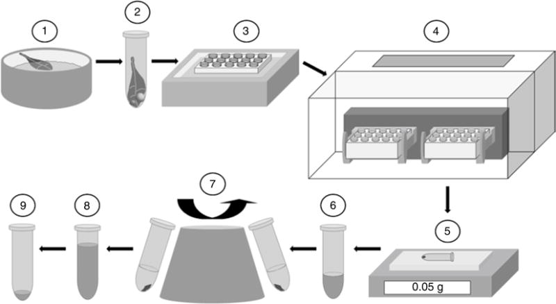
Sample preparation method B. (1) Flash freeze the plant tissue in liquid nitrogen, (2) transfer the plant tissue to a centrifuge tube containing the pre-chilled grinding balls, (3) transfer the centrifuge tube to a pre-chilled centrifuge tube holder in a liquid nitrogen bath, (4) place the centrifuge tube holder in the mixing chamber of the ball mill and start the grinding cycle, (5) weigh out 50 mg of the plant tissue, (6) add 500 μL of 13 mM ammonium acetate solution and mix thoroughly, (7) centrifuge and transfer the supernatant to a separate centrifuge tube, (8) repeat steps 6 and 7 twice and combine the three extracts, (9) freeze, freeze dry, then reconstitute the dried extract in 100 μL acetonitrile–water (1:1, v/v)

1. Pour liquid nitrogen into an appropriately sized freezer box until it is approximately a quarter full.

2. Immerse the cryogenic centrifuge tube holder (which is open at the base) in the liquid nitrogen. The holder will be pre-chilled when the nitrogen bath is no longer bubbling. Leave about a cm gap from the top of the centrifuge tube holder.

3. Pre-chill the stainless steel grinding balls (typically a 2 mm and a 4 mm ball are used) in liquid nitrogen that is housed in a clean cryogenic container.

4. Transfer a centrifuge tube to the pre-chilled centrifuge tube holder in the nitrogen bath. It should be noted that there will be liquid nitrogen in the holes of the centrifuge tube holder (as liquid nitrogen will enter from the base of the holder).

5. Wait until the nitrogen bath is no longer bubbling.

6. Quickly transfer the stainless steel grinding balls to a centrifuge tube in the pre-chilled centrifuge tube holder.

7. Harvest the plant tissue and flash freeze in liquid nitrogen.

8. Transfer the plant tissue to a centrifuge tube (containing the stainless steel grinding balls) in the pre-chilled centrifuge tube holder.

9. Place the centrifuge tube holder in the mixing chamber of the ball mill.

10. Start the grinding cycle and leave for 1 min.

11. Transfer the centrifuge tube holder to a freezer box containing dry ice.

12. Remove the steel grinding balls from the centrifuge tube.

13. Weigh out 50 mg of the homogenized/ground plant tissue in a centrifuge tube.

14. Add 500 μL of 13 mM ammonium acetate buffer in water (adjusted to pH 5.5 with acetic acid) to the plant tissue and mix thoroughly by vortexing.

15. Centrifuge at the highest speed of the bench-top microcentrifuge for 5 min at 4 °C.

16. Transfer the supernatant to a new centrifuge tube.

17. Repeat steps 14–16 twice (steps 14–16 are performed on ice).

18. Combine the three extracts together, freeze with liquid nitrogen and freeze dry.

19. Reconstitute the extract in 100 μL of the appropriate internal standards in acetonitrile–water (1:1, v/v).

3.3 IXC-IEC-ESI-TOF MS

A new column is flushed with 0.1 % formic acid in water overnight at a flow rate of 0.1 mL/min and at a temperature of 50 °C. This is to remove any contaminants from the previous mobile phase and to equilibrate the column(see ^{Note 15}). Before LC-ESI-TOF MS analysis, the column is flushed with 0.1 % formic acid for 30 min at a flow rate of 0.1 mL/min and at a temperature of 50 °C. The LC column compartment and autosampler thermostat temperatures are maintained at 50 °C and 4 °C, respectively. The sample injection volume used is 5–10 μL. The mobile phase is composed of 0.1 % formic acid in water and a flow rate of 0.6 mL/min is used throughout the analysis. The maximum backpressure that the LC column is able to tolerate is normally 200 bar (see ^{Note 16}). The HPLC system is coupled to a TOF MS with a 1:6 post-column split (see ^{Notes 17} and ¹⁸). In this experiment, LC-ESI-MS coupling is achieved using an orthogonal interface. Nitrogen gas is used as both the nebulizing and drying gas to facilitate the production of gas-phase ions. The drying and nebulizing gases are set to 11 L/min and 30 psi, respectively, and a drying gas temperature of 330 °C is used throughout. Fragmentor, skimmer and ion-guide rf voltages are set to 150 V, 50 V, and 170 V, respectively. ESI is conducted in the negative-ion mode with a capillary voltage of 3.5 kV. MS experiments are carried out in the full-scan mode (m/z 145–605) at 0.86 spectra per second for the detection of [M–H]⁻ ions. The instrument is tuned for a range of m/z 50–1,700. Prior to LC-ESI-TOF MS analysis, the TOF MS is calibrated with the manufacturers TOF tuning mix. Internal calibration of the TOF m/z axis is performed with the relevant reference masses provided by the instrument manufacturer (see ^{Notes 19–21}). A typical autosampler sequence consists of: blank → calibration curve → blank → samples → blank → calibration curve → blank. If the background noise (observed via the total ion chromatogram) is high, then more than one blank may be used at the start of the run.

1. Enter the required LC and MS parameters as well as the run sequence in the acquisition software. Normally the acquisition software will not allow the run sequence to be activated unless these parameters are saved. Once saved, the resulting method and the sequence work list can be used for future experiments.

2. Connect the mobile phase reservoir to the HPLC system.

3. Switch on the purge valve system.

4. Turn on a single HPLC pump.

5. Set the flow rate of the HPLC pump to 5 mL/min for 2 min. Purge the HPLC pump with the new mobile phase. Here the flow is directed to waste.

6. Turn off the HPLC pump.

7. Switch off the purge valve system. The flow is now directed to the column.

8. Change the flow rate to 1 or 2 mL/min depending on the HPLC system used (see ^{Note 22}).

9. Turn on the column compartment. The temperature is set to 50 °C.

10. Turn on the HPLC pump and observe the mobile phase emerging from the column compartment-to-column connection tubing.

11. Wait until the previous mobile phase has been completely replaced. One way of determining this is to test the pH of the emerging droplets (with a pH strip). If the pH is ≤3 then the previous mobile phase has been replaced. Another way is to observe the backpressure. That is, the stabilization of the back-pressure is a good indication that the previous mobile phase has been replaced.

12. Connect the guard and analytical column to the column compartment.

13. Set the flow rate to 0.1 mL/min.

14. Turn on the HPLC pump and collect the column effluent for waste disposal.

15. Wait until the backpressure has stabilized.

16. Increase the flow rate to 0.2, 0.3, 0.4, 0.5, and finally to 0.6 mL/min (waiting for the backpressure to stabilize after each incremental increase in flow rate).

17. Once the back pressure has stabilized, connect the calibrant delivery system to the MS.

18. Turn on the MS and calibrate the time-of-flight mass axis.

19. Then connect the HPLC system to the ESI-MS sprayer via connection tubing.

20. Start the run sequence.

21. The total run time is 20 min.

22. Representative results are shown in Fig. 6. Once the analysis is completed flush the column with the mobile phase at 0.1 mL/min for 30 min (at 50 °C). The column can now be stored for future use. Please refer to the manufacturer’s guidelines for the appropriate column cleaning and regeneration procedures.

Fig. 6.

IXC-IEC-ESI-TOF MS analysis of DXP pathway intermediates. Counts versus time (min). The data was acquired from 80 to 605 m/z

3.4 HILIC-ESI-quad MS

LC column compartment and autosampler thermostat temperatures are maintained at 30 °C and 4 °C, respectively. The sample injection volume used is 4 μL. The mobile phase is composed of (A) 50 mM ammonium carbonate in water (see ^{Note 23}) and (B) acetonitrile. Isocratic elution is achieved at 70 % B at a flow rate of 0.2 mL/min. The maximum backpressure that the LC column is able to tolerate is 200 bar. The HPLC system is coupled to a single quadrupole mass spectrometer MS with a 1:3 post-column split. In this experiment, LC-ESI-MS coupling is achieved using an orthogonal interface. Nitrogen gas is used as both the nebulizing and drying gas to facilitate the production of gas-phase ions. The drying and nebulizing gases are set to 10 L/min and 30 psi, respectively, and a drying gas temperature of 330 °C is used throughout. ESI is conducted in the negative-ion mode with a capillary voltage of 3.5 kV. MS experiments are carried out in the SIM mode (87, 169, 213, 215, 261, 277, and 520 m/z) at 3 s/cycle at a dwell time of 500 ms (or ≤1.2 s/cycle at a dwell time of 200 ms if faster scanning is required) for the detection of [M–H]⁻ ions. The instrument is tuned for a range of m/z 50–1,700 with the appropriate tuning mix provided by the manufacturer. A typical autosampler sequence consists of: blank → calibration curve → blank → samples → blank → calibration curve → blank.

1. Enter the required LC and MS parameters as well as the run sequence in the acquisition software.

2. Connect the mobile phase reservoir to the HPLC system.

3. Switch on the purge valve system.

4. Turn on both HPLC pumps.

5. Set the flow rate of HPLC pump A to 5 mL/min for ~2 min (i.e., until the backpressure stabilizes). Purge the HPLC pump with the new mobile phase. Here the flow is directed to waste.

6. Repeat step 5 for HPLC pump B.

7. Turn off both HPLC pumps.

8. Switch off the purge valve system. The flow is now directed to the column.

9. Reenter the appropriate mobile phase composition in the acquisition software (i.e., 30 % A and 70 % B).

10. Change the flow rate to 1 or 2 mL/min depending on the HPLC system used.

11. Turn on the column compartment. The temperature is set to 30 °C.

12. Turn on both HPLC pumps and observe the mobile phase emerging from the column compartment-to-column connection tubing.

13. Wait until the previous mobile phase has been completely replaced. To determine whether the previous mobile phase has been replaced, observe the pH of droplets (the pH should be ~9) and/or monitor the backpressure of the HPLC system.

14. Connect the guard and analytical column to the column compartment.

15. Set the flow rate to 0.1 mL/min.

16. Turn on the HPLC pump and collect the column effluent for waste disposal. The column can now be equilibrated with the starting mobile phase composition (i.e., 30 % A and 70 % B).

17. Once the backpressure has stabilized increase the flow rate to 0.2 mL/min.

18. Turn on the MS. Then connect the HPLC system to the ESI-MS sprayer via connection tubing.

19. Start the run sequence.

20. The total run time is 19 min.

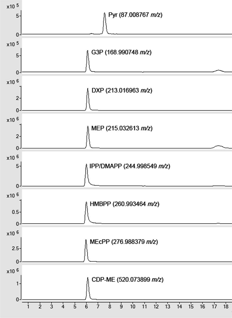
21. Representative results are shown in Fig. 7. Once the analysis is completed flush the column with 5 mM ammonium acetate in acetonitrile–water (8:2, v/v) at 0.1 mL/min for 20 min (at room temperature). The column can now be stored for future use. Please refer to the manufacturer’s guidelines for the appropriate column cleaning and regeneration procedures.

Fig. 7.

HILIC-ESI-quad MS analysis of DXP pathway intermediates. Counts versus time (min). The data was acquired in the SIM mode with pre-selected ions of 87, 169, 213, 215, 261, 277, and 520 m/z

References

- 1.Xiao Y, Savchenko T, Baidoo EEK, Chehab WE, Hayden DM, Tolstikov V, Corwin JA, Kliebenstein DJ, Keasling JD, Dehesh K. Retrograde signaling by the plastidial metabolite MEcPP regulates expression of nuclear stress-response genes. Cell. 2012;149:1525–1535. doi: 10.1016/j.cell.2012.04.038. [DOI] [PubMed] [Google Scholar]
- 2.Kirby J, Keasling JD. Biosynthesis of plant isoprenoids: perspectives for microbial engineering. Annu Rev Plant Biol. 2009;60:335–355. doi: 10.1146/annurev.arplant.043008.091955. [DOI] [PubMed] [Google Scholar]
- 3.Li Z, Sharkey TD. Metabolic profiling of the methylerythritol phosphate pathway reveals the source of post-illumination isoprene burst from leave. Plant Cell Environ. 2013;36:429–437. doi: 10.1111/j.1365-3040.2012.02584.x. [DOI] [PubMed] [Google Scholar]
- 4.Hunter W. The non-mevalonate pathway of isoprenoid precursor biosynthesis. J Biol Chem. 2007;282:21573–22177. doi: 10.1074/jbc.R700005200. [DOI] [PubMed] [Google Scholar]
- 5.Guidelines for use and care of Aminex® resin-based columns (LIT42 Rev D) Bio-Rad Laboratories, Inc; http://www.bio-rad.com/webroot/web/pdf/lsr/literature/LIT42D.PDF. [Google Scholar]
- 6.Harris DC. Quantitative chemical analysis. 6th. W.H. Freeman and Company; New York: 2003. [Google Scholar]
- 7.Gama MR, Silva RGD, Collins CH, Bottoli CBG. Hydrophylic interaction chromatography. Trends Anal Chem. 2012;37:48–60. [Google Scholar]
- 8.Buszewski B, Noga S. Hydrophilic interaction liquid chromatography (HILIC)—a powerful separation technique. Anal Bioanal Chem. 2012;402:231–247. doi: 10.1007/s00216-011-5308-5. [DOI] [PMC free article] [PubMed] [Google Scholar]
- 9.De Hoffman E, Stroobant V. Mass spectrometry principles and applications. 2nd. Wiley; New York: 2002. [Google Scholar]
- 10.Stewart II. Electrospray mass spectrometry: a tool for elemental speciation. Spectrochim Acta B. 1999;54:1649–1695. [Google Scholar]
- 11.Smyth WF. The use of electrospray mass spectrometry in the detection and determination of molecules of biological significance. TrAC Trends Anal Chem. 1999;18:335–346. [Google Scholar]
- 12.Smith JN, Flagan RC, Beauchamp JL. Droplet evaporation and discharge dynamics in electrospray ionization. J Phys Chem A. 2002;106:9957–9967. [Google Scholar]
- 13.Wilm MS, Mann M. Electrospray and Taylor-Cone theory, Dole’s beam of macromolecules at last? Int J Mass Spectrom Ion Proc. 1994;136:167–180. [Google Scholar]
- 14.Fenn JB. Ion formation from charged droplets: roles of geometry, energy, and time. J Am Soc Mass Spectrom. 1993;4:524–535. doi: 10.1016/1044-0305(93)85014-O. [DOI] [PubMed] [Google Scholar]
- 15.Fjeldsted J. Time-of-flight mass spectrometry. Technical overview. 2003 http://www.chem.agilent.com/Library/technicaloverviews/Public/5989-0373EN%2011-Dec-2003.pdf.
- 16.Willoughby R, Sheehan E, Mitrovich S. A global view of LC/MS: how to solve your most challenging analytical problems. 1st. Global View Publishing; Pittsburgh: 1998. [Google Scholar]
- 17.Skoog DA, Holler FJ, Nieman TA. Principles of instrumental analysis. 6th. Brooks Cole; USA: 2006. [Google Scholar]
- 18.Jhonstone RAW, Rose ME. Mass spectrometry for chemists and biochemists. 2nd. Cambridge University Press; Cambridge: 1996. [Google Scholar]
- 19.Smith RM, Busch KL. Understanding mass spectra—a basic approach. Wiley; New York: 1999. [Google Scholar]
- 20.Weickhardt C, Moritz F, Grotemeyer J. Time-of-flight mass spectrometry: state-of the-art in chemical analysis and molecular science. Mass Spectrom Rev. 1996;15:139–162. doi: 10.1002/(SICI)1098-2787(1996)15:3<139::AID-MAS1>3.0.CO;2-J. [DOI] [PubMed] [Google Scholar]
- 21.Guilhaus M. Principles and instrumentation in time-of-flight mass spectrometry—physical and instrument concepts. J Mass Spectrom. 1995;30:1519–1532. [Google Scholar]
- 22.McIntire D. Effect of resolution and mass accuracy on empirical formula confirmation and identification of unknowns. Technical overview. 2004 http://www.chem.agilent.com/Library/technicaloverviews/Public/5989-1052EN%2014-May-2004.pdf.