

Abstract
Motivation: Automated fluorescence microscopes produce massive amounts of images observing cells, often in four dimensions of space and time. This study addresses two tasks of time-lapse imaging analyses; detection and tracking of the many imaged cells, and it is especially intended for 4D live-cell imaging of neuronal nuclei of Caenorhabditis elegans. The cells of interest appear as slightly deformed ellipsoidal forms. They are densely distributed, and move rapidly in a series of 3D images. Thus, existing tracking methods often fail because more than one tracker will follow the same target or a tracker transits from one to other of different targets during rapid moves.
Results: The present method begins by performing the kernel density estimation in order to convert each 3D image into a smooth, continuous function. The cell bodies in the image are assumed to lie in the regions near the multiple local maxima of the density function. The tasks of detecting and tracking the cells are then addressed with two hill-climbing algorithms. The positions of the trackers are initialized by applying the cell-detection method to an image in the first frame. The tracking method keeps attacking them to near the local maxima in each subsequent image. To prevent the tracker from following multiple cells, we use a Markov random field (MRF) to model the spatial and temporal covariation of the cells and to maximize the image forces and the MRF-induced constraint on the trackers. The tracking procedure is demonstrated with dynamic 3D images that each contain >100 neurons of C.elegans.
Availability: http://daweb.ism.ac.jp/yoshidalab/crest/ismb2014
Supplementary information: Supplementary data are available at http://daweb.ism.ac.jp/yoshidalab/crest/ismb2014
Contact: yoshidar@ism.ac.jp
1 INTRODUCTION
Fluorescence microscopy imaging of live cells has been a powerful tool for studying cellular and molecular dynamics in many applications (Peng, 2008; Swedlow et al., 2009). Automated microscopes generate vast numbers of images of the observed cells, and the images are often in four dimensions of space and time. The cells in these images are densely distributed, move rapidly and are often similar in appearance. It is thus impossible in practice to manually track hundreds of such cells as their movement is captured in a sequence of images. This has led to growing interest in computational methods that can automatically detect and track multiple moving cells (Altinok et al., 2006, 2007; Gerlich et al., 2003; Hadjidemetriou et al., 2004; Jaqaman et al., 2008; Meijering et al., 2006; Shen et al., 2010; Smal et al., 2008a, b; Thomann et al., 2002).
The appearance of imaged cells can vary from globular to more complicated forms. They move independently, or sometimes their movement is coordinated. Cell tracking methods have been developed for particular cases of interest [see Meijering et al. (2012) for a comprehensive survey]. In general, tracking procedures consist of two steps: (i) relevant objects are segmented from the background in each frame by using, for example, the watershed algorithm (Grau et al., 2004; Malpica et al., 1997; Vincent and Soille, 1991), and (ii) each of the segmented objects is then linked to the nearest object in the subsequent frame (Hadjidemetriou et al., 2004; Meijering et al., 2006). To reduce the number of failures in the process of matching nearest neighbors, closeness is defined not only on the spatial distance between the objects, but also on other available information, such as variations in volume, morphology, intensity and other features (Meijering et al., 2012). The integration of such information is essential when the imaged cells move in a complex manner. However, in several studies, such information is limited or even unavailable. For instance, when fluorescent cells are much smaller than the optical resolution of microscopes, it is difficult to evaluate morphological features because most objects have similar appearances. This is especially true when the objects have inherently similar shapes, are closely spaced, and are barely distinguishable from the background. In such cases, tracking must be done using only the central coordinates of the cells.
This study tackles the problem of tracking many cells while relying only on the central coordinates. The cells of interest appear as slightly deformed ellipsoidal forms. In addition, they move rapidly in coordination with one another. Widely used tracking methods, such as nearest matching methods (Hadjidemetriou et al., 2004; Meijering et al., 2006), particle filters (Doucet et al., 2001; Khan et al., 2004; Smal et al., 2008a, b; Shen et al., 2010) and graph-based optimization (Jaqaman et al., 2008), often fail because trackers change from the followed target to a different one (turnover) or because two or more trackers coalesce on the same target during rapid moves. One way to overcome such difficulties is to utilize a spatiotemporal pattern of covariation for the moving cells. In conventional methods, in which the trackers follow each object individually, many such turnovers and coalescences occur in the transition of objects. In particular, when using nearest neighbor matching of segmented objects, the occurrence of only a few turnovers can trigger a series of many tracking failures. However, when cells are known to move in a coordinated way and the transition pattern is modeled, such errors can be corrected by successful trackers, which can return the failed trackers to their correct positions. In other words, unlike the independent tracking of multiple cells, the performance is enhanced by allowing the trackers to interact cooperatively by sharing the direction and distance of the moves.
The present method aims to improve the tracking performance by utilizing the spatiotemporal covariation of the moving cells. The proposed method relies on the kernel density estimation (KDE) (Silverman, 1986; Wand and Jones, 1986) and several optimization modules. It begins by using KDE to convert each image to a smooth, continuous density function in 3D space. The cells in the image are assumed to appear as slightly deformed ellipsoidal forms and to lie in the regions around the local maxima of the density functions. The tasks of detecting and tracking the cells are addressed by using hill-climbing algorithms for the continuous functions. For detecting the cells, we introduce a new optimization method, the repulsive parallel hill-climbing (RPHC) algorithm, which detects all of the existing local maxima and thus reduces the chances of failing to detect the darker and smaller objects. The trackers are initialized at the detected positions in the first frame. The tracking algorithm keeps them near the local maxima, which change with time. To prevent the trackers from turnovers and coalescences, we used a Markov random field (MRF) prior to model the spatial and temporal covariation of the moving cells. By using the MRF-induced cooperation, the present method tries to keep the trackers near to the varying local maxima of the density functions by optimizing the image forces under a constraint on the covariation of the objects. The present method is an extension of Smal et al. (2008b) and Khan et al. (2004), which proposed similar tracking methods based on the particle filter and MRF priors. They aimed to track the movements of several tens of targets interacting with each other. This study differs from their works in the prior construction as shown in later. In addition, this study is conducted for a much larger number of targets, e.g. several hundreds of cells, while the motions of targets are more strongly correlated than those considered by the previous studies. The tracking procedure will be demonstrated below with data that we acquired from live imaging of neuronal nuclei of Caenorhabditis elegans.
2 METHODS
2.1 Data
With confocal laser microscopy, live-cell imaging experiments were carried out to identify simultaneously multiple neurons of adult C.elegans. The neuronal nuclei of C.elegans were labeled with mCherry, a well-known red fluorescent protein (Shaner et al., 2004), which was fused to four nuclear localization signals and was expressed specifically in neurons. The microscope measured the intensities of this tracer in order to follow the positions and movements of the imaged objects. In this study, the following two types of data were analyzed.
DATA1. A set of static 3D gray-scale images was used to test the cell detection algorithm. Each image stack contained 148–200 neurons whose positions were identified manually by human observers in order to define the ground truth. Figure 1 shows a 3D image which consists of a 203 slice stack of images. The voxel-specific intensities wi were defined over a set of n voxels, where the total number of voxels was (x, y, z). According to the spatial distribution of the fluorescent protein within a nucleus, the appearance of each neuron can vary slightly in size and shape, and can be either ellipsoidal or somewhat more complicated. We obtained 10 datasets of this type.
DATA2. We obtained a time series of images for each time frame where T = 500. The data were used to assess the performance of the cell-tracking algorithm. At each frame t, the voxel-specific intensities were measured over n voxels We obtained three different datasets of this type. For each dataset, the total observational time was ∼3.25 min with 2.56 frames per second. In the series of experiments, a worm’s body was inserted and fixed to a polydimethylsiloxane-based microfluidic device tube attached to the microscope (Chronis et al., 2007), and there was no stimulation. Although sufficiently immobilized and attached to the device, the worm can slightly change its body posture in the field of view. As seen from Figure 2 and the video in Supplementary Material 1, the shift of the imaged neurons tends to be almost in parallel, retaining their relative positions, but some groups of neurons often move together in a direction that is slightly different from that of the others. These groups often exhibit significantly greater mobility than average. These dynamic properties are modeled and are automatically explored by using the MRFs. It is noted that there are no cell divisions during the experiments, and thus the present method is designed to have a fixed number of trackers.
Fig. 1.

Static 3D image of 157 neurons The white circles indicate the positions of the neurons, which were detected by expert human observers. Imaged cells appear as slightly deformed ellipsoids, as seen in the enlargement
Fig. 2.

Examples of dynamic image frames The top and bottom panels show the images at t = 30 and t = 34, respectively. The full movie is available in Supplementary Material 1
2.2 Outline of the method
The automated tracking procedure that we propose consists of four internal processing steps (see Figure 3 for a schematic view):
For each time frame t, use KDE to transform the 3D image to a continuous density function.
At the initial frame t = 1, detect all of the local maxima of the density function by using a hill-climbing algorithm. Identify the number g and the central coordinates of the imaged cell. The g trackers are initialized at those positions.
For each of the adjacent frames for track the centers of the cells by shifting the g trackers from to near the local maxima of the density function of the current frame t. This is done by maximizing the objective function that consists of the image force induced by the density function and the constraint on the transitions of the g trackers.
For each t, segment a region of each cell for which neighboring voxels will be allocated to the tracked cell center.
Fig. 3.

Outline of the proposed method. For each time frame, the 3D image is transformed to the continuous density function by using the KDE technique. Using the image at t = 1, a hill-climbing method for continuous functions is used to initialize the trackers’ positions at the local maxima of the density function. The tracking method then tries to keep the trackers near to the local maxima as they change with time in the subsequent images
2.3 KDE
KDE converts each digital image to a continuous density function. This aims to reduce image noises instead of using existing image blur filters, and to use optimization techniques designed for continuous objective functions in the subsequent processes.
For each t, the image It is converted to the density function p(x) as
| (1) |
For notational simplicity, the frame index t is omitted here. This is a mixture of the n Gaussian distributions, with each centered at a voxel position xi. The normalized voxel intensities wi comprise the mixing rates, which should sum to one. The function is continuous on Hence, hill-climbing algorithms for continuous functions can be used, and by repeating them many times with different initial values, the local maxima can be discovered. With this conversion, we can compute the gradient and the Hessian matrix at any and thus can identify the local maximum achieving the exact zero gradient while it is difficult to define accurately the local maximum for usual peak detection methods that rely on raw digital images.
To reduce the noise and artifacts in the images, it is important to control the covariance parameters of the kernel densities that comprise the bandwidth and the coordinate-specific dispersions in The density function becomes either over- or under-smoothed as the covariance components vary from larger to smaller values. Hence, the choice of these parameters has a strong influence on the ability to find the local maxima. In this study, we tuned the covariance parameters so that they were specifically optimized for analyzing the live-cell-imaging data that we measured. The coordinate-specific dispersions were fixed at and for DATA1 and DATA2, respectively. We chose these values in the following way; relatively smaller objects had been previously segmented from several images using the k-means clustering method as shown in Appendix B, and observed scale ratios in the three directions (x, y, z) were referred to determine these values. To determine the global scale h, we first isolated subimages that included tightly clustered cells from some of the target datasets, as shown in Figure 4. Here, the number of cells in each subimage was determined by expert human observers. By performing KDE with each subimage and using the cell-detection method described in the next subsection, we counted the number of local maxima that appeared in each grid point of width h (Figure 4). We then selected the value of h that yielded an appropriate number of local maxima; this was 0.52 and 0.97 for DATA1 and DATA2, respectively. These parameter values were applied to all the data of the same type.
Fig. 4.

Subimages containing several closely spaced cells were isolated from the given data (DATA1). For each subimage, the number of cells was identified by human observers. An appropriate value for the bandwidth h was chosen so that the number of local maxima of the density function was in agreement with the manually identified cell counts
In statistics, various methods for selecting the bandwidth have been established for multivariate cases, including the minimum-risk procedure based on the integrated mean square error and the cross-validation method [refer to Silverman (1986) and Wand and Jones (1986) for reviews]. These are still useful for image processing, given trivial modifications (conventional procedures presume equal mixing rates, , and hence it is necessary to derive variants for unequal mixing rates when using the existing techniques). However, we decided not to use any of the existing procedures because numerical tests showed they have a tendency of yielding over- or under-estimates.
In subsequent steps, it is necessary to compute the kernel density many times. This becomes a computational bottleneck due to the large number of basis functions, e.g. n = 2, 621, 440 for DATA2. Therefore, for each 3D image, we reduced n by conducting a threshold operation in which voxel intensities <5% upper quantile were set to zero. To control the threshold level, many other techniques can be applied, for example, Otsu’s algorithm for binarization of gray-scale images (Otsu, 1979). See Sezgin and Sankur (2004) for a survey of threshold algorithms. In addition, Chapter 4 of Silverman (1986) provides some techniques that can be implemented to reduce the computational cost of KDE.
2.4 Cell count and detection
Once a kernel density estimate has been obtained for the initial frame, an exhaustive search is then conducted to find the local maxima. The number and the positions of the local maxima can be used to estimate the number of cells and their positions, respectively. Starting from an arbitrary initial position the following recurrent formula produces a sequence that converges to a local maximum:
| (2) |
At step s, the position is renewed to by taking the weighted average of xi, Points xi that are closer (as determined by the normalized weights to the current position have a greater influence on the new position. In a way similar to the expectation-maximization algorithm for a Gaussian finite mixture, it can be proved that this hill-climbing procedure produces a non-decreasing sequence of and converges to the nearest local maxima. In a context of cluster analyses, a mode-finding method of this type was described in Hinneburg and Gabriel (2007), which also provided some techniques for speeding up the computation. Equation (2) can be derived as a trivial variant of their algorithm.
Finding all of the local maxima requires repeating the search from many different initial positions because many searches may converge to the same local maximum that may correspond to a significantly bright and large object. Figure 5 shows an experimental result in which 500 different initial positions were generated uniformly over 3D space (DATA1), and the 500 independent trials found 118 different local maxima. Among the 157 cells that were manually identified, 41 of the darker and smaller cells rest undetected.
Fig. 5.

Result of 500 independent trials of the hill-climbing algorithm, Equation (2), with different initial values. The red boxes indicate the 116 true positives (TPs) that were detected by both the hill-climbing method and the human observers. The white boxes indicate the 41 false negatives (FNs) that were overlooked by the hill-climbing method. The yellow boxes indicate two false positives (FPs) that were detected by the hill-climbing method
In order to improve the detection performance, the RPHC algorithm was used. Given m initial seeds, the method computes the following recursive formula in parallel for
| (3) |
where is an indicator function that takes the value one if the argument is true and is zero otherwise. The set denotes a local ellipsoidal region of volume v centered at which defines a neighboring area of the k-th object at step s. This equation differs from Equation (2) in the weight components The voxel position xi and the corresponding kernel density are removed from the operation of renewing the j-th position by assigning if the voxel is already occupied by the neighboring areas of the other positions Hence, the j-th process tends to deviate from the others due to the repulsion acting on (see Figure 6). It is expected that the m search processes will tend to climb different hills, and that with a single parallel run, they will therefore converge on different local modes.
Fig. 6.

Schematic view of the RPHC algorithm. (1) The two search processes (A and B) are climbing the same local maximum. (2) When renewing process A, the kernel densities within a neighboring area of process B are removed, which changes the shape of the hill. Because of this, process A will move toward a different hill
In our implementation, the neighbor is given by the ellipsoidal region whose volume vs is reduced from a positive value to zero in stages as the step s increases. The Hessian matrix is set to the covariance matrix H, which approximates the local curvature in a neighborhood of ψ. A method for computing the Hessian matrix is described in Appendix A. The volume decreases linearly as with a small positive β until it converges to zero. It should be noted that the iteration must converge to zero volume in order to remove the bias caused by the repulsion of the nonzero vs. The initial volume v0 and the rate of decrease β should be determined by the cell volumes. Appendix B describes a procedure for obtaining initial estimates of the cell volumes and setting the parameters for the reduction process.
In Supplementary Material 2, we provide a demonstration movie that shows the search process of the RPHC algorithm applied to synthetic data in which 96 cells were allocated at equally spaced grid points. For the purpose of demonstration, 120 initial positions were allocated within a small region near a corner of the 3D space. For an initial period of time, the 120 search processes repelled each other, and they gradually diffused over the entire space due to the repulsion. At convergence, they had determined all 96 local maxima. More detailed tests with real data will be shown in Section 3.
2.5 Cell tracking
After applying the RPHC algorithm to the image in the first frame t = 1, the trackers were placed at the positions of the g non-overlapping objects in which redundant positions were removed from the m points of convergence. The objective of multi-object tracking is to keep the trackers targeting the local maxima, which change with time. There are two kinds of tracking errors to be considered: (i) different trackers merge to the same target, and (ii) a tracker switches to a different target.
To prevent the trackers from merging and switching, we use the spatiotemporal covariation of the movement of the cells. As a result, the j-th tracker is encouraged to transit from to in conjunction with the other trackers that belong to a set , called the neighbor set of j. To be specific, we build a transition model based on an MRF as
| (4) |
where The direction and distance of the move are correlated with those of for the neighboring trackers The degree of correlation is controlled by the magnitude of the variance of the Gaussian noise As becomes smaller, the higher correlations are induced to the transition of and The construction of will be described below.
With the transition model of Equation (4) and the current guess the tracking method explores the new by finding the maximum of the conditional density with respect to
| (5) |
where denotes the square of the Mahalanobis distance with the covariance matrix Σ. The first component is the Gibbs distribution with the temperature whose energy involves the logarithmic transformation of the current kernel density. This yields an image force on the tracker which is then attracted to a high-probability region of the KDE. The MRF model in Equation (4) defines the second component, which enforces the spatiotemporal covariation and eliminates the overlaps when renewing the trackers’ positions.
To seek the solution for we conduct the following recursion for and until convergence;
| (6) |
In the above, the components are averaged with the assigned weights The weighted average of the voxel coordinates in the first term of Equation (6) arises from maximizing only the image force, i.e. the Gibbs distribution in the first component of Equation (5). Maximizing the second component of Equation (5) derives the remaining components that work to shift toward the same direction as the other for
To define the graphical structure,  we explore a minimum spanning tree of the g trackers. The Σ-scaled Mahalanobis distances between the previous positions
  are assigned as the edge costs of the complete graph on the g vertices. For each frame, Prim’s algorithm (Prim, 1957) is used to find the spanning tree that has the lowest total cost. We then assign the inverse of each edge cost to the noise variance as
  . Because
  and
and 
 are invariant under any multiplication of γ and
 by an arbitrary constant, it is enough to determine the ratio between γ and
  in order to compute Equation (6). We controlled the ratio value manually while inspecting the tracking results.
Smal et al. (2008b) and Khan et al. (2004) proposed the similar ideas of using MRF priors based on the particle filter in order to track the movement of several tens of targets. Their MRF priors rely only on the current positions of objects; coalescence of trackers can be avoided by penalizing tracked positions that are closely spaced. Instead, the present MRF prior describes a different type of motion coherency, the direction and distance of the transition between two successive frames among neighboring objects. This model is designed specifically for our data.
2.6 Segmentation: Bayes’ allocation rule
We address the segmentation task as follows; the voxels that surround each central coordinate were allocated to the tracked object successively. For a given position at each time t, we define the region of interest (ROI), as the collection of voxels lying in a high-probability region or a cluster of the KDE. The following procedure explores the ROIs by allocating each voxel to one of based on Bayes’ rule.
Round off to the nearest integer each of the tracked positions within the 3D image space of interest.
Set a threshold level which is used for the Bayes’ allocation rule.
Initialize the ROIs by for
- Execute the following steps until convergence:
- For each voxel position, say xi, compute the probability of allocating i to as
- The voxel i is allocated to if and only if and .
- Return to step (a) until no further change is made in renewing any
3 RESULTS AND DISCUSSION
3.1 Cell detection
The RPHC algorithm was applied to each of the 10 datasets (DATA1) in which 148–200 manually identified cells were imaged. For the hill-climbing, 500 initial values were allocated uniformly over the entire 3D space. The results were compared to those of the hill-climbing without repulsion [500 independent trials of Equation (2)] and the watershed segmentation (Grau et al., 2004; Malpica et al., 1997; Vincent and Soille, 1991). For the watershed segmentation, we used the MATLAB function watershed after performing a noise-reduction process (smooth3 in MATLAB). We then computed the center of each segmented region to define a point estimate of the cell position. For each method, a detected position was called a true positive if it was within a radius of 5 pixels of a manually identified cell position; otherwise, it was called a false positive. A manually identified position that was overlooked by a computational method was called a false negative. The detection performances for the 10 datasets are summarized in Table 1. On average, the inclusion of the repulsive force in the parallel hill-climbing process increased the rate of true positives by >10%, with only a slight increase in the rate of false positives (see the results of the independent hill-climbing and RPHC algorithm in Table 1). Figure 7 shows the 151 positions detected by the RPHC algorithm, and Figure 8 shows the ROIs resulting from the Bayes’ voxel allocation rule. For this dataset, the RPHC algorithm resulted in 138 true positives, 13 false positives and 19 false negatives, whereas those of the independent hill-climbing algorithm were 116 true positives, 2 false positives and 41 false negatives.
Table 1.
Comparison of the cell-detection performances
| Independent_500 | Independent_1000 | RPHC | Watershed | |
|---|---|---|---|---|
| False positive rate | 0 (0) | 0 (0) | 0.0301 (0.0305) | 0.3453 (0.1182) |
| True positive rate | 0.7190 (0.0257) | 0.7383 (0.0287) | 0.8041 (0.0362) | 0.8021 (0.0381) |
The columns indicate the independent hill-climbing algorithm with 500 and 1000 initial positions (Independent_500 and Independent_1000), the RPHC algorithm (RPHC) and the watershed segmentation (Watershed). Rates of false positives and true positives were averaged over the 10 datasets (DATA1). The values in parentheses indicate the standard deviations.
Fig. 7.

Result of the RPHC algorithm on DATA1. The red, white and yellow boxes indicate TPs (138), FNs (19) and FPs (13), respectively (the definitions of TP, FN and FP are given in the caption of Figure 5)
Fig. 8.

ROIs (151) obtained by performing the Bayes’ allocation rule on DATA1
The hill-climbing algorithm is ensured theoretically to converge to a local maximum in spite of the presence or absence of repulsion. In this task, it is important to discover all existing local maxima, and the decision whether or not each identified position is a false positive or true positive is to be left up to expert knowledge or an additional post-processing step. Indeed, some positions called the false positives were identified as cells the human observers failed to find. In this regard, the RPHC algorithm that identified much larger numbers of local maxima outperformed the independent search. It should be remarked that the independent search even with 1000 initial seeds only identified ∼73% of the manually identified positions on average (Table 1), and thus showed no significant improvements while the computation time was doubled.
On the other hand, as indicated by many previous studies, the watershed segmentation exhibited obvious oversegmentation, as shown in Table 1. For example, for the dataset shown in Figure 9, the watershed segmentation resulted in 245 detected objects, whereas the number of cells estimated by human observers was 157 and that by the RPHC algorithm was 151.
Fig. 9.

Centers of ROIs (245) obtained by the watershed segmentation on DATA1. The red, white and yellow boxes indicate TPs (122), FNs (35) and FPs (123), respectively (the definitions of TP, FN and FP are given in the caption of Figure 5)
Figure 8 shows the ROIs resulting from the Bayes’ voxel allocation rule. It is apparent that most of the ROIs were segmented successfully, while some cells were segmented at unnatural boundaries. In the segmentation method, the boundary of each segment resulted from the positional relationship of the cells, since any overlap was not permitted in the segmentation rule. Thus some ROIs were separated by the unnatural boundary when the cells are located closely. This drawback is yet to be addressed.
3.2 Cell tracking
The tracking algorithm is first illustrated with one of the three dataset in DATA2. For the initial frame, the trackers were initialized at the positions of 111 objects that had been detected by the RPHC algorithm. The tracking algorithm was then run for 500 frames. As shown in the full movie of the tracking process (Supplementary Material 3), in all frames, the trackers’ positions can be seen to be attracted to neighboring areas of the local modes of the KDEs. In particular, turnover and coalescence of the tracked positions occurred rarely, other than for a fraction of the 111 trackers. The tracking process indicates that it is reasonable to represent the adjacency relationship of cells by a tree. Also, the minimum spanning tree (MST) varied in structure only slightly throughout the tracking process.
To assess the performance on the three datasets in a quantitative way, we defined the ground truth in the following way: each original image sequence was joined to the time-reversal set, and thus we have of the length The performance was evaluated on the number of trackers that returned to the initial positions at the final frame I1. A tracker was called a success if it was in a radius of 5 pixels of the initial position in the final frame. As an additional criterion, we used the number of merges in trackers in the final frame. We conclude upon the results summarized in Table 2 that the present method could track 70–91% of the moving objects.
Table 2.
Performances of the tracking method on the three datasets (D1–D3) in DATA2
| Number of trackers | Return rate | Non-overlaping rate | |
|---|---|---|---|
| D1 | 111 | 0.9136 | 0.9454 |
| D2 | 121 | 0.7520 | 0.9504 |
| D3 | 113 | 0.7011 | 0.8230 |
The columns indicate the number of trackers and the two performance measures: (i) the rate of trackers that returned to the correct positions (return rate) and (ii) the rate of non-overlapping trackers that successfully avoided coalescence (non-overlaping rate).
One major difficulty arose during a phase in which the cells exhibited large mobility. In such a case, methods that rely only on the nearest-neighbor matching are prone to serious tracking errors. Figures 10 and 11 show the transitions of 111 individual trackers at a phase of the tracking processes of the proposed method and the particle filter algorithm (Jaqaman et al., 2008; Smal et al., 2008b; Shen et al., 2010). Our own program for the particle filter was developed with reference to Arulampalam et al. (2002), which is substantially based upon the principle of nearest neighbor matching. Figure 11 and the full movie in Supplementary Material 4 illustrate the tracking failure of the particle filter. As shown in Figure 11, many trackers failed to follow the targets when many of the cells underwent significantly large moves. In addition, the full movie shows that the errors accumulated with time due to the absence of error-correction functionality.
Fig. 10.
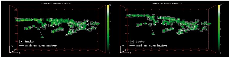
Results of the proposed tracking method. The left and right figures show the results obtained at t = 30 and t = 34, respectively. The white boxes indicate the tracked positions. The white lines indicate the minimum spanning tree. The full movie of this tracking process is available at Supplementary Material 3
Fig. 11.

Results of the particle filter. The left and right figures show the results obtained at t = 30 and t = 34, respectively. The white boxes indicate the tracked positions. The white lines indicate the minimum spanning tree. The full movie of this tracking process is available at Supplementary Material 4
4 CONCLUDING REMARKS
This article presented a series of image processing steps for tracking many moving cells in a series of 3D images. The appearance of the cells was almost homogeneous deformed ellipsoids. The method relied only on the central coordinates of the objects, since any other features such as morphology, volume or intensity were very limited. The basis of the method was KDE. By using KDE to transform the images, the tasks of cell detection and tracking could be addressed in a unified manner that involved the two hill-climbing methods designed for continuous probability density functions. In particular, we presented two novel techniques; the RPHC algorithm for cell detection, and multi-cell tracking based on the MRF. The former initialized trackers in the first frame at the coordinates of the detected cells, and the latter maintained them in mutually exclusive positions at the bright areas of images that evolved with time. In live-cell imaging experiments, cells often move relative to one another. The use of MRFs might enhance the tracking performance, since successful trackers bring erroneous trackers back to their correct positions. The present method relies on this key idea.
This article concludes with some remarks on the practical use of the current method and limitations yet to be overcome.
All the steps in the present method rely on the local maxima of the KDE. An obvious drawback arises from the fact that unwanted local maxima are present due to noise introduced into the image processing. Therefore, it is considerably important to conduct pre- and post-processing in order to reduce such artifacts. In the application of this method to our data, we found that it would have been useful to remove some of the very small segmented objects. Other ways to avoid detection of unwanted local maxima include the removal of closely paired or extremely dark objects.
In this article, our interest was limited to cases where there are no cell divisions, and thus the present method was designed to have fixed number of trackers. However, it is important to extend the current method to account for merges and splits of cells as many previous studies have been motivated.
In statistics, many methods exist for the selection of bandwidth, for example, Silverman’s rule of thumb and several cross-validation methods [see Silverman (1986) for a review]. We used Silverman’s rule of thumb, in which a multivariate normal distribution was used for the reference density (Scott, 1992), and the leave-one-out cross validation based on the log-likelihood risk (Silverman, 1986), and although the results are not shown here, these caused significant under- and overestimates, respectively.
The underlying assumption behind the tracking method is that the movements of most of the cells are highly correlated according to shifts in the worm’s body. However, the tracking method would still be applicable when the positions of the cells change smoothly over time, since the graphical structure of the MRF is reconstructed sequentially at each time frame.
ACKNOWLEDGEMENT
The authors thank Manami Kanamori for important contributions to the experiments. We thank Masayuki Henmi for useful discussions and comments.
Funding: The CREST program ‘Creation of Fundamental Technologies for Understanding and Control of Biosystem Dynamics ' of Japan Science and Technology Agency (JST).
Conflict of Interest: none declared.
Appendix A GRADIENT AND HESSIAN OF KDE
The exact formulae for the gradient and the Hessian matrix can be derived by noting the analogy of Equation (1) to the conventional Gaussian finite mixture:
As a reference for the derivation, see, for example, Carreira-Perpinan (2000).
Appendix B PRIMARY ESTIMATE OF CELL VOLUME AND DESIGN OF VOLUME REDUCTION PROCESS
First, a sample of size is resampled from the n voxels, with probabilities Suppose that we have a primary guess on the number of cells present in an image. Performing the k-means algorithm on the sample brings a segmentation of the voxels into non-overlapping clusters. A cluster of voxels can be an estimate for a cell-embedded region. Principal component analysis was applied to the within-cluster voxels, and the product of the resulting three eigenvalues, gives an estimate for the cell volume. Finally, the 5% upper-quantile of the estimated volume was set to v0. The rate of the volume reduction was chosen as so that the volume converges to zero at the end of 500 iterations.
REFERENCES
- Altinok A, et al. Activity analysis in microtubule videos by mixture of hidden Markov models. CVPR. 2006;2:1662–1669. [Google Scholar]
- Altinok A, et al. Model based dynamics analysis in live cell microtubule image. BMC Cell Biol. 2007;8:S4. doi: 10.1186/1471-2121-8-S1-S4. [DOI] [PMC free article] [PubMed] [Google Scholar]
- Arulampalam MS, et al. A tutorial on particle filters for online nonlinear/non-Gaussian Bayesian tracking. IEEE Transact. Signal Process. 2002;50:174–188. [Google Scholar]
- Carreira-Perpinan MA. Mode-finding for mixtures of Gaussian distributions. IEEE Transacti. Patt. Anal. Mach. Intell. 2000;22:1318–1323. [Google Scholar]
- Chronis N, et al. Microfluidics for in vivo imaging of neuronal and behavioral activity in Caenorhabditis elegans. Nat. Methods. 2007;4:727–731. doi: 10.1038/nmeth1075. [DOI] [PubMed] [Google Scholar]
- Doucet A, et al. Particle filters for state estimation of jump Markov linear systems. IEEE Transact. Signal Process. 2001;49(3):613–624. [Google Scholar]
- Gerlich D, et al. Quantitative motion analysis and visualization of cellular structures. Methods. 2003;29:3–13. doi: 10.1016/s1046-2023(02)00287-6. [DOI] [PubMed] [Google Scholar]
- Grau V, et al. Improved watershed transform for medial image segmentation using prior information. IEEE Transact. Med. Imaging. 2004;23:447–458. doi: 10.1109/TMI.2004.824224. [DOI] [PubMed] [Google Scholar]
- Hadjidemetriou S, et al. Automatic quantification of microtubule dynamics. I S Biomed Imaging. 2004;1:656–659. [Google Scholar]
- Hinneburg A, Gabriel H-H. Denclue 2.0: Fast clustering based on kernel density estimation. LNCS. 2007;4723:70–80. [Google Scholar]
- Jaqaman K, et al. Robust single-particle tracking in live-cell time-lapse sequences. Nat. Methods. 2008;5:695–702. doi: 10.1038/nmeth.1237. [DOI] [PMC free article] [PubMed] [Google Scholar]
- Khan Z, et al. An MCMC-based particle filter for tracking multiple interacting targets. LNCS. 2004;3024:279–290. [Google Scholar]
- Malpica N, et al. Applying watershed algorithms to the segmentation of clustered nuclei. Cytometry. 1997;28:287–297. doi: 10.1002/(sici)1097-0320(19970801)28:4<289::aid-cyto3>3.0.co;2-7. [DOI] [PubMed] [Google Scholar]
- Meijering E, et al. Tracking in molecular bioimaging. IEEE Signal Process. Mag. 2006;23:46–53. [Google Scholar]
- Meijering E, et al. Methods for cell and particle tracking. Methods Enzymol. 2012;504:183–200. doi: 10.1016/B978-0-12-391857-4.00009-4. [DOI] [PubMed] [Google Scholar]
- Otsu N. A threshold selection method from gray-level histograms. IEEE Transact. Syst. Man Cybernet. 1979;9:62–66. [Google Scholar]
- Peng H. Bioimage informatics: a new area of engineering biology. Bioinformatics. 2008;24:1827–1836. doi: 10.1093/bioinformatics/btn346. [DOI] [PMC free article] [PubMed] [Google Scholar]
- Prim RC. Shortest connection networks and some generalizations. Bell Syst. Tech. J. 1957;39:1389–1401. [Google Scholar]
- Scott DW. Multivariate Density Estimation: Theory, Practice, and Visualization. New York: John Wiley; 1992. [Google Scholar]
- Sezgin M, Sankur B. Survey over image thresholding techniques and quantitative performance evaluation. J. Electronic Imag. 2004;13:146–165. [Google Scholar]
- Shaner NC, et al. Improved monomeric red, orange and yellow fluorescent proteins derived from Discosoma sp. red fluorescent protein. Nat. Biotechnol. 2004;22:1567–1572. doi: 10.1038/nbt1037. [DOI] [PubMed] [Google Scholar]
- Shen H, et al. Automatic tracking of biological cells and compartments using particle filters and active contours. Chemom. Intell. Lab. Syst. 2010;82:276–282. [Google Scholar]
- Silverman BW. Density Estimation for Statistics and Data Analysis. London: Chapman and Hall; 1986. [Google Scholar]
- Smal I, et al. Multiple object tracking in molecular bioimaging by Rao-Blackwellized marginal particle filtering. Medi. Image Anal. 2008a;12:764–777. doi: 10.1016/j.media.2008.03.004. [DOI] [PubMed] [Google Scholar]
- Smal I, et al. Particle filtering for multiple object tracking in dynamic fluorescence microscopy images: application to microtubule growth analysis. IEEE Transact. Med. Imag. 2008b;27:789–804. doi: 10.1109/TMI.2008.916964. [DOI] [PubMed] [Google Scholar]
- Swedlow JR, et al. Bioimage informatics for experimental biology. Ann. Rev. Biophys. 2009;38:327–346. doi: 10.1146/annurev.biophys.050708.133641. [DOI] [PMC free article] [PubMed] [Google Scholar]
- Thomann D, et al. Automatic fluorescent tag detection in 3D with super-resolution: application to the analysis of chromosome movement. J. Microscopy. 2002;208:49–64. doi: 10.1046/j.1365-2818.2002.01066.x. [DOI] [PubMed] [Google Scholar]
- Vincent L, Soille P. Watersheds in digital spaces: an efficient algorithm based on immersion simulations. IEEE Transact. Pattern Anal. Machi. Intell. 1991;13:583–598. [Google Scholar]
- Wand MP, Jones C. Kernel Smoothing. London: Chapman and Hall; 1986. [Google Scholar]