MR PROSTATE SEGMENTATION VIA DISTRIBUTED DISCRIMINATIVE DICTIONARY (DDD) LEARNING

Abstract

Segmenting prostate from MR images is important yet challenging. Due to non-Gaussian distribution of prostate appearances in MR images, the popular active appearance model (AAM) has its limited performance. Although the newly developed sparse dictionary learning method[1, 2] can model the image appearance in a non-parametric fashion, the learned dictionaries still lack the discriminative power between prostate and non-prostate tissues, which is critical for accurate prostate segmentation. In this paper, we propose to integrate deformable model with a novel learning scheme, namely the Distributed Discriminative Dictionary (DDD) learning, which can capture image appearance in a non-parametric and discriminative fashion. In particular, three strategies are designed to boost the tissue discriminative power of DDD. First, minimum Redundancy Maximum Relevance (mRMR) feature selection is performed to constrain the dictionary learning in a discriminative feature space. Second, linear discriminant analysis (LDA) is employed to assemble residuals from different dictionaries for optimal separation between prostate and non-prostate tissues. Third, instead of learning the global dictionaries, we learn a set of local dictionaries for the local regions (each with small appearance variations) along prostate boundary, thus achieving better tissue differentiation locally. In the application stage, DDDs will provide the appearance cues to robustly drive the deformable model onto the prostate boundary. Experiments on 50 MR prostate images show that our method can yield a Dice Ratio of 88% compared to the manual segmentations, and have 7% improvement over the conventional AAM.

1. INTRODUCTION

Magnetic resonance (MR) image is becoming more and more popular in the prostate related clinical studies[3]. Among these studies, the segmentation of prostate gland is a fundamental and important step. It can not only provide the volume of prostate gland, which is an important diagnostic measurement, but also pave the way to other image-based diagnosis/treatment tasks, i.e., prostate cancer staging and MR-guided radiotherapy planning. Accordingly, extensive research has been conducted on automatic segmentation of prostate from MR images.

As one of the most successful segmentation algorithms, active shape/appearance model (ASM/AAM) becomes a natural choice to tackle this segmentation problem. For example, Toth et al. [4] proposed a landmark-free AAM-based method and further created a deformable registration framework to fit a trained appearance model to a new image. In the recent MICCAI PROMISE challenge, quite a few methods were also designed based on ASM/AAM. For example, to prevent boundary leakage, Kirschner et al. [5] presented a probabilistic ASM (PASM) which can adapt a statistical shape model to a larger subspace than the one spanned by the principal eigenvectors used in the standard ASM. Although these methods proved the feasibility to automatic prostate MR segmentation, they all confront an inherent limitation of ASM/AAM, which assumes that both shape and appearance statistics of the targeted object follow the Gaussian distributions. This assumption is not valid in prostate MR due to the complicated neighboring structures along prostate boundary, highly inhomogeneous magnetic fields, and large inter-patient variations (c.f., Fig. 1).

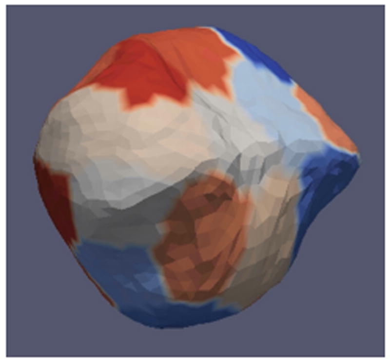
Fig. 1.

Complicated non-Gaussian distribution of appearance features (gradient, intensity) in MR prostate images.

Recently, sparse learning theory has gained high attentions in computer vision [1, 2]. Instead of assuming any parametric model, sparse learning theory aims to learn a parametric-free dictionary to represent signals of the same class, and thus opens a door to model prostate appearance with the complicated statistical distribution. However, since sparse learning aims to “represent one class (i.e., prostate)” rather than “distinguish one class from others (i.e., prostate vs. non-prostate)”, the learned sparse dictionary may not be able to well differentiate prostate from non-prostate tissues, which may eventually affect the final segmentation results.

In this paper, we improve the conventional sparse learning with a discrimination technique and further integrate it with the deformable model to segment prostate in MR images. Hence, sparse dictionaries can be learned to identify prostate tissues and provide appearance cues for driving our deformable model more effectively. Specifically, the conventional sparse learning will be improved in three aspects to boost the tissue discriminative power. First, mRMR feature selection [6] is performed to constrain the dictionary learning always in a discriminative feature space. Second, LDA is employed to assemble residuals from different dictionaries for optimal separation between prostate and non-prostate tissues. Third, a set of local dictionaries is learned for tissue differentiation in the local regions along prostate boundary. In the application stage, these learned local dictionaries will provide effective appearance cues to robustly drive the deformable model onto the prostate boundary.

2. METHODS

2.1. Problem Statement

The previous success of ASM/AAM mainly comes from the joint use of both appearance and shape priors by assuming their separate Gaussian distributions. However, due to large variations and complicated distributions of prostate appearance and shape in MR images (c.f., Fig. 1), the basic assumption of Gaussian distribution is invalid and the ASM/AAM is not able to segment prostate MR accurately.

To alleviate the limitation in modeling of shape prior, we will employ the Sparse Shape Composition (SSC) approach [2] which learns a sparse dictionary to represent prostate shapes in the most compact and effective way. Since SSC does not assume any parametric model of shape statistics, it can effectively model prostate shape priors, which may not follow a Gaussian distribution.

However, dictionary learning cannot be directly borrowed to model the complicated appearance statistics, since the objectives of shape and appearance modeling are inherently different. Specifically, shape prior modeling aims to represent shape instances in the same class, which is a “one-class representation” problem. On the other hand, appearance modeling targets to distinguish different tissues (prostate vs. non-prostate), which is essentially a “two-class classification” problem. As the conventional dictionary learning is designed for one-class representation, the learned dictionary might not have strong tissue differentiation capability, which is critical for accurate segmentation.

To boost the discriminative power of the learned dictionaries, we propose here a novel learning scheme, namely the Distributed Discriminative Dictionary (DDD) learning. As shown in Fig. 2, it includes three novel strategies, i.e., sparse learning with feature selection, discriminative ensemble of representation residuals, and distributed learning, all of which are detailed below.

Fig. 2.

Diagram of Distributed Discriminative Dictionary (DDD) learning framework. (a) A schematic explanation of distributed discriminative dictionaries, with each taking charge of tissue differentiation in a local region. (b) Diagram of training a discriminative dictionary, including key components of mRMR feature selection, sparse representation, and LDA learning.

2.2 Sparse dictionary learning with mRMR feature selection

Notations

Denote f_x as the appearance feature vector of a voxel x, containing the Histogram of Oriented Gradients (HOG), Haar, intensity and gradient features calculated in the neighborhood of x. F is a feature matrix that is concatenated by feature vectors of voxel set.

To model appearance characteristics of voxels in F, the standard dictionary learning method optimizes the following objective function.

$$\underset{\mathit{D},\mathit{C}}{\min }{\Vert \mathit{F}-\mathit{DC}\Vert }_2\mathrm{s}.\mathrm{t}.{\Vert {\mathit{c}}_i\Vert }_0\le K{\forall }_i$$ (1)

Here, C is the coefficient matrix, with its ith column c_i denoting the sparse coefficients of the ith appearance feature vector in F. D is the learned sparse dictionary that encodes appearance characteristics of voxels in F.

Using the standard dictionary learning, e.g., K-SVD [7], we can learn two dictionaries D_P and D_N on feature matrices of prostate voxels, F_P, and non-prostate voxels, F_N, respectively. Although D_P and D_N can well represent the appearance characteristics of F_P and F_N, they might not be able to separate prostate from non-prostate voxels due to the lack of considering the inter-class information in Eq. 1. More specifically, since the optimization of Eq. 1 only targets to the reconstruction error and the sparsity constraint, the discriminant information for separating prostate and non-prostate tissues are not guaranteed to be captured in the learned dictionaries.

In order to preserve the discriminant information in the learned dictionaries (D_P and D_N), the dictionary learning should be constrained in a discriminative feature space. In our study, we employ mRMR algorithm [6] to build a discriminative feature space. Compared to other feature selection methods [8], which only select individual features with highest discrimination, mRMR minimizes the redundancy of the selected features as well. Thus, the selected features span a discriminant sub-space, in which prostate and non-prostate tissues can be well separated.

Mathematically, mRMR first converts feature matrices F_P and F_N to F̂_P and F̂_N, which only contain selected discriminative features. Then, K-SVD [7] is applied to learn D̂_P and D̂_N on F̂_P (prostate) and F̂_N (non-prostate), respectively. Since the dictionary learning is constrained in a discriminative space, the learned dictionaries will always contain discriminant information. Consequently, D̂_P and D̂_N encode distinctive appearance characteristics, which can be used to classify prostate and non-prostate tissues.

2.3. Discriminative ensemble of representation residuals

To exploit the learned dictionaries for tissue differentiation, we first employ the standard sparse coding algorithm. Denote f̂_x as the feature vector that only includes the selected features of a voxel x. D̂ = [D̂_P, D̂_N] is a matrix concatenated by the two learned dictionaries. Sparse coding of f̂_x can be formulated as below:

$${\min }_{\mathit{\alpha }}{\Vert {\widehat{\mathit{f}}}_{\mathit{x}}­\widehat{\mathit{D}}\mathit{\alpha }\Vert }_2^2+\lambda {\Vert \mathit{\alpha }\Vert }_1$$ (2)

where α = [α_P, α_N] denote the sparse coefficients corresponding to the two learned dictionaries. In this way, the appearance features of x are represented by two different bases from D̂_P and D̂_N. Their corresponding representation residual vectors R_P(x) and R_N(x) can also be:

$$R_P(x)={\widehat{f}}_x­{\widehat{D}}_P{\alpha }_P;R_N(x)={\widehat{f}}_x­{\widehat{D}}_N{\alpha }_N$$ (3)

Intuitively, for a prostate voxel, its appearance should be better approximated by atoms in D̂_P than atoms in D̂_N, i.e., ∥R_P(x)∥₂ < ∥R_N(x)∥₂. Therefore, one can simply compare ∥R_P(x)∥₂ and ∥R_N(x)∥₂ to determine if voxel x belongs to prostate. However, for tissue classification, the residuals of some features might be more important than others. Therefore, ∥ ∥₂, which weights each feature equally, is not the best metric to separate prostate from other tissues.

To achieve better classification, we propose to learn a linear classifier in the residual space using Fisher-LDA. Specifically, given a set of prostate and non-prostate training samples, the parameters of the classifier are calculated as:

$$\mathit{\omega }=\underset{\mathit{\omega }}{\mathrm{arg\; max}}\frac{{\mathit{\omega }}^T{\mathit{S}}_{\mathit{B}}\mathit{\omega }}{{\mathit{\omega }}^T{\mathit{S}}_{\mathit{W}}\mathit{\omega }},c=\mathit{\omega }·[({\mu }_P(\mathit{R})+{\mu }_N(\mathit{R}))/2.0]$$ (4)

Here, R =[R_P, R_N] denotes the residual space. S_B and S_W are the inter-class and the intra-class scatter matrices in R. μ_P (.) and μ_N (.) denote the average residuals of prostate and non-prostate samples, respectively.

By integrating Eq. 3 into the LDA classifier, we have a tissue score function h(x). For any voxel x under study, h(x) predicts the likelihood of x belonging to prostate based on its appearance f̂_x.

$$h_{(\mathit{x})}=\mathit{sig}(\mathit{\omega }·[{\widehat{\mathit{f}}}_x­{\widehat{\mathit{D}}}_{\mathit{P}}{\mathit{\alpha }}_{\mathit{P}},{\widehat{\mathit{f}}}_{\mathit{x}}­{\widehat{\mathit{D}}}_{\mathit{N}}{\mathit{\alpha }}_{\mathit{N}}]-c)$$ (5)

where sig(·) denotes the sigmoid function. D̂_P and D̂_N are the two learned dictionaries with their corresponding sparse coefficients α_P and α_N optimized in Eq. 2.

In Eq. 5, elements in the residual vectors are assigned with different weights to optimally separate prostate from non-prostate tissues. In other words, LDA provides a discriminative ensemble of residual elements for better tissue differentiation. As shown in our experiments, it exhibits much better performance compared to the conventional dictionary-based classification.

2.4. Distributed dictionary learning

In the two above-proposed strategies, dictionary learning has been effectively exploited to separate prostate from other tissues. However, it still confronts challenges from the large appearance variations along prostate boundary (c.f., Fig 2(a)). It is worth noting that the appearance variations within local regions are relatively small, which should be exploited to further improve the performance of tissue differentiation.

To this end, we design a “divide-and-conquer” learning strategy. Specifically, the deformable model is divided into M sub-surfaces corresponding to M local regions along prostate boundary (c.f., Fig. 3) {S_i ∣ i =1, ⋯, M}. This can be achieved by using the vertices clustering method proposed in [2], which ensures the appearance variations around each sub-surface are small (c.f., Fig. 2(a)). In this way, each sub-surface S_i can be attached by a pair of local dictionaries, ${\widehat{\mathit{D}}}_{\mathit{P}}^i$ and ${\widehat{\mathit{D}}}_{\mathit{N}}^i$, learned from samples extracted around S_i. Due to smaller appearance variations around S_i, these local dictionaries can better encode local appearance characteristics, and thus achieve more accurate tissue classification.

Fig. 3.

The partition of our deformable model. Sub-surfaces are indicated by different colors.

After performing this local learning, we now have a set of local tissue score functions {h_i(x) ∣ i = 1, ⋯ M}, each of which has the same form as in Eq. 5 but with different local dictionaries ${\widehat{\mathit{D}}}_{\mathit{P}}^i$ and ${\widehat{\mathit{D}}}_{\mathit{N}}^{\mathit{i}}$. In the application stage, each h_i (x) only generates tissue scores of voxels around the ith sub-surface, S_i. These local tissues scores are used as appearance cues to guide and drive the sub-surface S_i onto the prostate boundary. The deformed surface will be further constrained by the prostate shape priors formulated as sparse shape composition (SSC) [2, 9]. Thus, dictionary-guided deformation and SSC-based shape refinement can be iteratively performed until convergence. See [2, 9] for more details of the deformable segmentation framework.

3. EXPERIMENTS

Our method was evaluated on the MICCAI challenge data “PROMISE12”, which includes 50 T2-weighted MR images (20 for training and 30 for testing).

We first evaluated tissue classification performance of the proposed Distributed Discriminative Dictionary (DDD) learning. For comparison, we also implemented other two methods based on two different dictionary learning schemes: 1) Global Standard Dictionary (GSD): a pair of global dictionaries learned by the standard dictionary learning method; 2) Distributed Standard Dictionary (DSD): a set of distributed dictionaries learned by the standard dictionary learning method. As shown in Fig. 4, DDD achieves the best tissue classification accuracy with the area under curve (AUC) as 0.90, while the AUCs of GSD and DSD methods are 0.72 and 0.85, respectively. It is worth noting that these three methods are different only in the “discriminative” and “distributed” strategies, which shows the efficacy of our proposed strategies in accurate tissue classification.

Fig. 4.

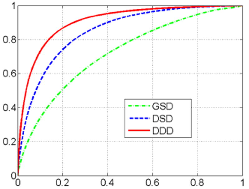
ROC curves of tissue classification using different methods.

We further evaluated the accuracy of our method in prostate segmentation. For comparison, besides the two dictionary learning-based methods as mentioned above, we also include three variants of ASM/AAM based method, ASM (guided by image gradients), PASM [5] and AAM [10]. Table 1 reports the mean and standard deviation (Std) of Dice ratio and average surface distance (ASD)[11] between automatic segmentation and manual segmentation. Again, our method achieves the best performance among all methods. Results on two typical examples are also shown in Fig. 5, for four different methods.

Table 1.

Mean value and standard deviation (Std) of Dice ratio and average surface distance (ASD) between algorithm outputs and ground truth for all comparison methods.

		ASM	PASM[5]	AAM[10]	GSD	DSD	DDD
Dice	Mean	0.74	0.77	0.81	0.78	0.82	0.88
	Std	0.09	0.23	0.12	0.08	0.06	0.03
ASD (mm)	Mean	4.41	4.10	—	3.82	2.83	1.86
	Std	1.45	7.81		1.21	0.88	0.74

Fig. 5.

Visual comparisons of segmentation results from 4 different methods. Red and yellow contours denote manual and automatic segmentations, respectively.

4. CONCLUSION

We have presented a novel method to segment prostate in MR images. To address the challenges from complicated appearances of prostate, we design a novel Distributed Discriminative Dictionary (DDD) learning to extract appearance characteristics in a non-parametric, discriminative, and local fashion, and further integrate it with deformable model to segment prostate from MR images. Experiments on MICCAI “PROMISE12” dataset show that our method can achieve much better segmentation results than the conventional ASM/AAM and also the standard sparse dictionary learning-based methods.

References

- 1.Wright J, Yang AY, Ganesh A, et al. Robust face recognition via sparse representation. IEEE PAMI. 2009;31(no 2):210–227. doi: 10.1109/TPAMI.2008.79. [DOI] [PubMed] [Google Scholar]
- 2.Zhang S, et al. Deformable segmentation via sparse representation and dictionary learning. MIA. 2012;16(no 7):1385–1396. doi: 10.1016/j.media.2012.07.007. [DOI] [PubMed] [Google Scholar]
- 3.Hricak H, et al. Imaging Prostate Cancer: A Multidisciplinary Perspective1. Radiology. 2007 Apr;243(no 1):28–53. doi: 10.1148/radiol.2431030580. [DOI] [PubMed] [Google Scholar]
- 4.Toth R, Madabhushi A. Multifeature landmark-free active appearance models: application to prostate MRI segmentation. IEEE TMI. 2012;31(no 8):1638–1650. doi: 10.1109/TMI.2012.2201498. [DOI] [PubMed] [Google Scholar]
- 5.Kirschner M, Jung F, Wesarg S. Automatic prostate segmentation in MR images with a probabilistic active shape model. MICCAI PROMISE’12 Challenge. 2012:28–35. [Google Scholar]
- 6.Peng H, Long F, Ding C. Feature selection based on mutual information criteria of max-dependency, max-relevance, and min-redundancy. IEEE PAMI. 2005;27(no 8):1226–1238. doi: 10.1109/TPAMI.2005.159. [DOI] [PubMed] [Google Scholar]
- 7.Aharon M, Elad M, Bruckstein A. K-SVD: an algorithm for eesigning overcomplete dictionaries for sparse representation. IEEE TSP. 2006;54(no 11):4311–4322. [Google Scholar]
- 8.Jain A, et al. Feature selection: evaluation, application, and small sample performance. IEEE PAMI. 1997;19(no 2):153–158. [Google Scholar]
- 9.Zhang S, et al. Towards robust and effective shape modeling: Sparse shape composition. MIA. 2012;16(no 1):265–277. doi: 10.1016/j.media.2011.08.004. [DOI] [PubMed] [Google Scholar]
- 10.Maan B, et al. Prostate MR image segmentation using 3D active appearance models. MICCAI PROMISE’12 Challenge. 2012:44–51. [Google Scholar]
- 11.Gao Y, et al. Prostate segmentation by sparse representation based classification. Medical Physics. 2012;39(no 10):6372–6387. doi: 10.1118/1.4754304. [DOI] [PMC free article] [PubMed] [Google Scholar]