Model Simulations of the Bay of Fundy Gyre: 1. Climatological Results

Abstract

The characteristics of a persistent gyre in the mouth of the Bay of Fundy are studied using model simulations. A set of climatological runs are conducted to evaluate the relative importance of the different forcing mechanisms affecting the gyre. The main mechanisms are tidal rectification, and density-driven circulation. Stronger circulation of the gyre occurs during the later part of the stratified season (July–August and September–October). The density-driven flow around the gyre is set-up by weak tidal mixing in the deep basin in the central Bay of Fundy and strong tidal mixing on the shallow flanks around Grand Manan Island and western Nova Scotia. Retention of particles in the Gyre is controlled by the residual tidal circulation, increased frontal retention during stratified periods, wind stress, and interactions with the adjacent circulation of the Gulf of Maine. Residence times longer than 30 days are predicted for particles released in the proximity of the gyre.

1. Introduction and Background

While the circulation of the Gulf of Maine has been intensively studied for several decades [Bigelow, 1927; Brooks, 1985; Brown and Irish, 1992; Lynch et al., 1997; Pettigrew et al., 2005], the corresponding understanding of the dynamics of the adjacent Bay of Fundy is more limited. The circulation of the Bay of Fundy is subject to strong tides, especially the M₂ tidal constituent, resulting in tidal ranges of up to 8 meters at the mouth of the Bay and 16 meters at the head [Garrett, 1972; Greenberg, 1983]. Typical depth-averaged tidal current magnitudes of 0.8 – 1.2 ms⁻¹ over the deeper part of the Bay of Fundy basin and 1 – 2 ms⁻¹ over the shallow flanks at the mouth have been described [Godin, 1968; Greenberg, 1983; Brooks, 1994; Hannah et al., 2001]. The barotropic residual circulation is dominated by tidal rectification with flow into the Bay of Fundy along the southeastern side and flow out of the Bay along the northwestern side [Bigelow, 1927; Godin, 1968; Greenberg, 1983]. The density structure is the result of the basic balance between tidally-driven mixing and stratification due to surface heating [Garrett et al., 1978]. The general baroclinic circulation of the Bay remains poorly described.

The presence of counter-clockwise flow in the lower Bay of Fundy has been inferred from several past observations. Watson [1936] suggested the possibility of a counter-clockwise flow to explain dynamic height calculations from hydrography. Fish and Johnson [1937] and Hachey and Bailey [1952] suggested a similar possibility to explain surface drift bottle returns. Lauzier [1967] suggested a similar mechanism to explain sea-bed drifter trajectories. Finally, Godin [1968] presented the results of several current meters and proposed a schematic of the flow that included a gyre in the central Bay of Fundy. Observations of the full structure and extent of this circulation are incomplete.

Based on the limited available information, the proposed basic structure of the flow suggest a counter-clockwise circulation with flow into the Bay along the Nova Scotia coast, northwest flow across the Bay, flow out of the Bay along the New Brunswick coast and eastern Grand Manan Island, closing the Gyre with southeast flow across the entrance of the Bay [Hachey and Bailey, 1952; Dickie, 1955; Godin, 1968]. Parts of the circulation associated with this hypothetical gyre (except the southeast flow at the mouth of the Bay) were described even in earlier contributions [Mavor, 1922; Bigelow, 1927, 1928]. The exchange of waters associated with the proposed position of the gyre with the surrounding waters has been shown to have a high interannual variability [Hachey, 1934]. Early coarse-resolution model simulations of the lower Bay region did not find an expression of this gyre [Greenberg, 1979, 1983]. Brooks [1994] described a small cyclonic eddy in the lower Bay under condition of strong mixing. Lynch et al. [1997] presented climatological solutions that begin to resolve it, and the gyre was present seasonally but sensitive to the presence of their near-field boundary. More modern simulations with finer grids seem to capture some representation of it [Xue et al., 2000; Hannah et al., 2001].

The biological implications of the presence (or lack there of) of the gyre has been described in several studies. Aspects of the circulation of the gyre were proposed to explain the retention of several organisms: phytoplankton [Gran and Braarud, 1935], zooplankton [Fish and Johnson, 1937], scallop larvae [Dickie, 1955], lobster larvae [Campbell, 1985], larval cod [Hunt and Neilson, 1993], and the toxic dinoflagellate Alexandrium fundyense [McGillicuddy et al., 2005]. Several studies about A. fundyense populations in the Gulf of Maine [White and Lewis, 1982; McGillicuddy et al., 2005] suggest the Bay of Fundy gyre as a relevant structure for the retention of cells and their efflux into the Maine Coastal Current. Blooms of this dinoflagellate occur annually in the Bay of Fundy and its effect on shellfish has been recorded since 1935 [Martin and White, 1988]. The fact that few cells are found in the central and northern Bay of Fundy, while all life stages of the organism are found near the mouth of the Bay, suggest a possible retention associated with the gyre [White and Lewis, 1982; Martin and White, 1988; McGillicuddy et al., 2005].

Although the presence of the Bay of Fundy gyre is firmly entrenched in many conceptual models of physical and biological processes in the region, there has not yet been a systematic study of the seasonal mean circulation in this feature. Therefore, this model-based work focuses on the circulation in the mouth and lower Bay of Fundy (Figure 1). We describe the general structure of the feature as well as its seasonal variability. The forcings controlling the dynamics of the gyre are separated and its relative importance is evaluated. The retention characteristics for different periods during the stratified season are estimated and compared.

Figure 1.

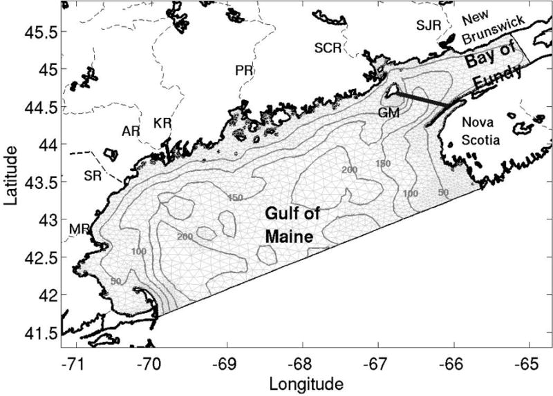
Map of the study region showing the model domain of the Gulf of Maine and Bay of Fundy. The thick black line indicates the position of a transect across the mouth of the Bay. The seven main rivers in the model domain are indicated with thin dashed lines: Merrimack (MR), Saco (SR), Kennebec (KR), Androscoggin (AR), Penobscot (PR), St. Croix (SCR), and St. John (SJR). GM stands for Grand Manan Island. The bottom topography contours of 50, 100, 150, and 200 meters are included.

2. Methods

2.1. Simulations

A set of climatological simulations are conducted to evaluate the relative importance of the forcing mechanisms in the Gyre. The period of interest focuses on the times when the presence of a Gyre has been suggested in previous studies [Dickie, 1955; Godin, 1968], from March to October. This long period is divided into four 60-day periods as in previous work [Naimie et al., 1994; Lynch et al., 1996]: March–April, May–June, July–August, and September–October. March–April is a transition period with high river discharge and the stratified season includes the other three periods. The simulations use the dominant M₂ tidal forcing, climatological atmospheric forcing (wind stress and heat flux), climatological river discharge, up-stream boundary conditions, and baroclinic pressure gradients from climatological temperature and salinity [Naimie et al., 1994]. In order to separate the effects of the different forcing mechanisms for each period, the experiments include 1) (Case T) a barotropic simulation to evaluate the effect of the tidal residuals (no wind, uniform mass field), 2) (Case T+M) a simulation with tides, mass field variations and heat flux (no wind), 3) (Case T+M+W) a simulation that includes winds, heat flux, tides, and baroclinic structure (no rivers), and 4) (Case T+M+W+R) a simulation with all the forcings included.

An approximation of the effects of the different forcings is calculated by differencing the various climatological solutions. The effect of the tidal residual circulation is therefore given by simulation Case T. The wind effect is approximated by subtracting simulation Case T+M from simulation Case T+M+W. The density (mass field) effect is estimated by subtracting simulation Case T from simulation Case T+M. Finally, the river effect is given by subtracting Case T+M+W from simulation Case T+M+W+R.

2.2. Model

The Quoddy model [Lynch and Werner, 1991] used in these simulations has been widely applied in the Gulf of Maine and adjacent areas [Lynch et al., 1996, 1997, 2001; Naimie, 1996; Proehl et al., 2004; He et al., 2005]. Quoddy is a three-dimentional, fully nonlinear, prognostic, tide-resolving, finite element model. Vertical mixing of subgrid-scale processes is parameterized using turbulence closure from Mellor and Yamada [1982].

The domain includes most of the Gulf of Maine from Cape Cod to southwestern Nova Scotia and north up to the vicinity of the head of the Bay of Fundy using realistic topography (Figure 1). The finest horizontal resolution is 2–3 km near the coast and it increases to around 8 km in the deep basin of the Gulf of Maine.

2.3. Inputs

Initial conditions are specified from the Gulf of Maine digital temperature and salinity climatology [Lynch et al., 1996]. These climatological fields have been used and tested in several previous studies of the Gulf of Maine circulation [Lynch et al., 1997; He et al., 2005]. Along the Bay of Fundy boundary, climatological M₂ tidal currents are prescribed along the boundary [Lynch and Naimie, 1993; Lynch et al., 1996]. The M₂ tide dominates the current and transport variability due to the shallow nature of the Bay along that boundary. The residual conditions along the Bay boundary are specified from climatology currents [Lynch et al., 1996], but correcting the velocities so that the mean residual transport across the entire boundary is zero. The “open-ocean” boundary conditions in the Gulf of Maine are imposed as sea surface elevation from climatological tidal and residual elevations [Lynch et al., 1996].

Atmospheric forcing is consistent with previous model studies of the Gulf of Maine and Georges Bank regions [Naimie et al., 1994; Lynch et al., 1996]. The wind stress used for each period is: March–April, 0.047 Pa 121° from true north (NW); May–June, 0.014 Pa 49° (SW); July–August, 0.014 Pa 51° (SW); and September–October, 0.019 Pa 146° (NW). The heat flux is the same used in Naimie et al. [1994] and Lynch et al. [1996, 1997], and is consistent with other climatological values for the Gulf of Maine region [Mountain et al., 1996].

Climatological river discharge data from archived U.S. Geological Survey and Water Survey of Canada stream gauge stations are compiled for the seven main rivers in the model domain (Figure 1): Merrimack, Saco, Kennebec, Androscoggin, Penobscot, St. Croix, and St. John. The associated river transport is imposed in the model domain area closest to the location of the measurement station. The volume flux of the St. John river (the closest river to the mouth of the Bay and the most relevant to the dynamics of the Gyre) in March–April is comparable to the values used by Brooks [1994] for the spring freshet (∼ 3 × 10³ m³s⁻¹) and smaller than the 30-year annual mean [Apollonio, 1979] during the rest of the periods.

Preliminary spin-up simulations are conducted for each period during 10 tidal cycles to achieve spin-up of the tides, rivers and climatological density fields. Model outputs at the end of the spin-up are saved and used as a hot start for the present simulations. The model is then run prognostically for another 20 tidal cycles and the output from the last tidal cycle is analyzed. By that point, mixing and flow stability have been achieved with changes between consecutive tidal cycles smaller than 1%. The temperature and salinity fields remain close to climatological magnitudes (variations due to mixing) except near river mouths, where the vertical salinity structure as a result of fresh water inputs controls the stratification especially during the March–April period.

3. Results

3.1. General Structure

The depth-averaged velocity for the May–June climatological period in the region surrounding the mouth of the Bay of Fundy (simulation Case T+M+W+R) shows the presence of the Gyre (Figure 2a). The Gyre exhibits two different paths in the northern region with a short central path following the 125m isobath and a longer path extending up to the 75m isobath. Another important feature is the strong flow convergence at the mouth of the Bay of Fundy (Figure 2a). The north flow circulating around western Nova Scotia splits around the 150m isobath creating two branches: one turning east into the Bay to form the eastern side of the Bay of Fundy Gyre, while the other turns west to feed the Maine Coastal Current. A similar separation occurs on the other side of the Gyre, where the strong south flow over the shoals southeast of Grand Manan Island splits in two branches: the first is a significant contribution to the Coastal Current, while the second represents the southern extent of the Bay of Fundy Gyre.

Figure 2.

Depth-averaged residual velocity for May–June climatological simulations: (a) Case T+M+W+R includes tidal residual, river, wind and baroclinic effect. (b) Case T (tidal residual). (c) Effect of climatological winds (Case T+M+W minus Case T+M). (d) Effect of the climatological density field (Case T+M minus Case T). Color scale represents depth-averaged speed (ms⁻¹).

The tidal residual circulation (simulation Case T) is one of the main contributors to the total Gyre dynamics (Figure 2b). The short central path of the Gyre that follows the 125m isobath, except in the proximity of Grand Manan Island, is driven by tidal rectification. The high velocities to the south of Grand Manan Island are the result of tidal rectification as well. The wind effect on the Gyre dynamics in the climatological simulations is small (Figure 2c). The low intensity winds during the summer months result in reduced averaged wind stress. The effect of river discharge on the depth-averaged velocity for the May–June period is relatively small as well and will be described in Section 3.2.

The baroclinic effect associated with the mass field is approximated by subtracting simulation Case T+M minus simulation Case T (Figure 2d). The mass field contributes to the recirculation in the northern part of the Gyre by controlling the flow associated with the longer path that approximately follows the 75m isobath in the northern part. The baroclinic effect also represents a significant contribution to the strength of the circulation in the southern and central part of the Gyre.

The subtraction of the climatological solutions to evaluate the effects of wind and baroclinicity is an approximation to the real effects of these forcings. The simulations are prognostic and non-linear, therefore, under conditions where strong non-linearities are certainly present, linear subtraction only gives a partial idea of their relative influences. Additional simulations are conducted (not shown) forced only with climatological density field or with climatological wind, and using prescribed averaged mixing from the Case T+M+W+R simulation. The results from these alternative simulations are substantively similar to the results from the linear subtraction, but the later are considered a more accurate representation of the wind and baroclinic effects because of the inclusion of the strong time-varying tidal mixing.

Observational data for a systematic quantitative validation of the presented climatological model velocities does not exist. Watson [1936], using dynamic height, estimated surface velocities of up to 0.3 ms⁻¹ east of Grand Manan and 0.2 – 0.25 ms⁻¹ west of Nova Scotia. Fish and Johnson [1937] and Hachey and Bailey [1952] estimated residual currents using drift bottle returns with velocities of 0.1 ms⁻¹ east of Grand Manan, 0.07 – 0.1 ms⁻¹ in areas corresponding with the northwestern part of the Gyre, and less than 0.02 ms⁻¹ elsewhere. Godin [1968], using three current meters, observed near-surface (5–13 meters) velocities of 0.2 – 0.25 ms⁻¹ west of Nova Scotia, 0.4 ms⁻¹ east of the St. John river mouth, and 0.15 – 0.25 ms⁻¹ in the center of the Bay in the northern part of the Gyre. Detided ADCP velocities observed during four recent cruises (May 2005, June 2007, May 2007, and June–July 2007) are consistent with the described structure of the Gyre and will be presented in a companion hindcast study.

A schematic of the residual circulation associated with the Bay of Fundy Gyre and the surrounding areas is presented in Figure 3. The main components of the Gyre include the strong tidal residual in the eastern and western edge of the Gyre and the relatively weaker tidal residual flow in the north (around the 125m isobath). The baroclinic effect extends much further into the Bay up the 75m isobath and its influence controls the circulation in the southern edge of the Gyre. The exchange with the surrounding areas is modified by the intense north flow west of Nova Scotia and its contribution to the Maine Coastal Current.

Figure 3.

Basic schematic of the circulation associated with the Bay of Fundy Gyre and its different forcing mechanisms. The strong tidal residual in both the east and west side of the mouth of the Bay is shown in dark blue, while in light blue, the weaker north component of the tidal residual around the 125m isobath. The baroclinic effect is included in red. The circulation in the Gulf of Maine associated with the north flow west of Nova Scotia and its connection to the Maine Coastal Current and the Bay of Fundy is presented in green. The exchange between the Gyre and the Coastal Current around the 100m isobath is shown in yellow.

3.2. River discharge

Previous model studies have described the effects of river discharge on the circulation of the Gulf of Maine and Bay of Fundy regions [Brooks, 1994; Xue et al., 2000]. One-third of the total mean freshwater contribution to the gulf is provided by the St. John river in New Brunswick just northeast of Grand Manan Island [Apollonio, 1979; Brooks, 1994], with its spring freshet being much larger than the annual mean. The relatively fresher water creates a bulge near the estuary mouth producing a near-surface clockwise circulation and resulting in a current flowing south with the coast to the right [Chao and Boicourt, 1986; Brooks, 1994]. The low-salinity flow joins the East Maine Coastal Current and continues flowing southwestward along the Maine coast [Brooks and Townsend, 1989; Brooks, 1994; Lynch et al., 1997; Pettigrew et al., 1998].

The effect of the St. John river discharge on the dynamics of the Bay of Fundy gyre has not been considered in previous studies. During the March–April period the described spring freshet has significant effects especially on surface circulation (Figure 4). The March–April surface salinity is largely affected by fresh water in the western side of the Bay from the St. John mouth to areas east of Grand Manan (not shown). Anticyclonic circulation associated with the fresh water bulge develops near the mouth of the river with current magnitudes of 0.2 – 0.25 ms⁻¹ (Figure 4a,d). The modeled velocities are consistent with estimates by Brooks [1994]. The spring freshet effect on depth-averaged velocity is much smaller (Figure 4e). Differences between the simulation including (Case T+M+W+R) and not including (Case T+M+W) rivers are generally less than 0.02 ms⁻¹. The anticyclonic circulation near the St. John mouth and the southwestward current along the coast are shown. During the March–April period, the effects on the Bay of Fundy gyre circulation are a slight increase of the flow along the northern edge of the gyre and an increase (0.01 ms⁻¹) of the flow east of Grand Manan Island.

Figure 4.

(a) Surface velocity for simulation Case T+M+W+R for the March–April period. (b) Depth-averaged velocity for simulation Case T+M+W+R for March–April. (c) Depth-averaged velocity for Case T+M+W+R for July–August. (d) Effect of river discharge on the surface velocity for the March–April period (Case T+M+W+R minus Case T+M+W). (e) Effect of river discharge on the depth-averaged velocity for March–April. (f) Effect of river discharge on the depth-averaged velocity for July–August. Color scales represent surface (a and d) or depth-averaged (b, c, e, and f) speeds (ms⁻¹). Color and vector scales change between panels.

The river effect on the depth-averaged circulation during the stratified season (May–October) is even smaller as a result of the weaker river discharge. The depth-averaged velocity difference for July–August (Figure 4f) is smaller than 0.01 ms⁻¹ even near the mouth of the St. John river. Therefore, considering the small effect of river discharge on depth averaged velocity, the schematic of the stratified season residual circulation associated with the Bay of Fundy Gyre (Figure 3) presented in Section 3.1 remains valid.

3.3. Seasonal variability

The seasonal variability is studied by comparing model simulations for the four different periods in which the Gyre has been described: March–April, May–June, July–August and September–October. In this section, the simulations that used the full forcing (river, atmospheric, tidal and baroclinic) are compared.

The depth-averaged velocities in the mouth of the Bay of Fundy for the entire stratified season (May–October) are quite similar, being weaker during the transition period of March–April. The differences between May–June velocities and the two later periods (July–August and September–October) are less than 0.01 ms⁻¹ for most of the mouth and central Bay of Fundy (Figures 2a and 4c). In the Gulf of Maine region, the July–August period has a stronger Maine Coastal Current associated with increased stratification (Figure 4c). The strength of the depth-averaged velocities during March–April (Figure 4b) is smaller than during May–June (Figure 2a) in the areas associated with the Gyre, especially in the shallow area south of Grand Manan Island where the March–April velocities are ∼ 0.05 ms⁻¹ smaller.

In order to extend our focus beyond the intensity of the currents, the extent of the counter-clockwise flow is considered using transport stream functions for the different periods (Figure 5). The estimated transport stream functions are consistent with the values for the Gulf of Maine region [Shore et al., 2000; Hannah et al., 2001]. Lowest values are estimated during March–April, peak values during summer (July–August) and a slight decrease during fall (September–October) in the Gulf of Maine, but not in the Bay of Fundy [Hannah et al., 2001]. An estimate of the extent of the continuous counter-clockwise flow is indicated by the completely closed streamline of 0.11 Sv. By this metric, the May–June period (Figure 5b) exhibits the largest extent, but the difference with later periods is minimal. The strength of the transport stream function associated with the gyre is greatest during the September–October period (Figure 5d, peak streamline of 0.2 Sv), but the values are similar during the last 3 periods (May through October). The weakest gradient (corresponding with weakest flow) and peak value (0.16 Sv) corresponds to the March–April period. The observed inter-decadal variability in the transport stream functions [Loder et al., 2001; Hannah et al., 2001] could be, in fact, larger than the described variability during the stratified season (May–September).

Figure 5.

Depth-integrated transport streamlines in units of Sverdrups (Sv) for four different periods: (a) March–April, (b) May–June, (c) July–August and (d) September–October. The streamline is zero at the coast, with increasing positive values on the left looking downstream as in Hannah et al. [2001]. The grey lines represent bottom topography contours of 50, 100, and 150 meters.

While the depth-averaged velocities during the summer months show only slight differences between the different periods, the surface velocity exhibits higher variability. During May–June the strongest along-isobath flow inside the Bay is estimated, while July–August presents a strong south to north cross-Bay flow component across the 150m isobath (not shown). This surface flow is associated with maximum near-surface stratification during the July–August period. The weakening of the stratification during September–October results in increased along-isobath flow in the Bay.

3.4. Vertical structure

The vertical structure of the flow (Figure 6) inside the Bay of Fundy Gyre is shown along a transect across the Bay (Figure 1). Large tidal vertical velocities are estimated for this area, but we focus on the residual vertical and tangential (cross-Bay) mean velocities evaluated as the detided Eulerian mean over the last tidal cycle. Brooks [1994] presented a similar vertical section located to the north of the current transect. The structures and magnitudes of the vertical and cross-Bay velocities presented herein are consistent with the results of Brooks [1994] except near the bottom, where their “slip” boundary condition limited the development of the appropriate bottom boundary layer. The maximum vertical speed is on the order of 10⁻⁴ ms⁻¹ representing a vertical displacement of 10 md⁻¹. The secondary circulation associated with the Gyre includes two recirculation cells: 1) a strong persistent cell in the western side of the transect, with near-bottom westward flowing upwelling from the 150m to the 50m isobath, weaker eastward flowing upwelling up to 20 meters, eastward flow at that depth and weak downwelling at the center of the basin; 2) a weaker highly variable cell in the eastern side, with near-bottom upwelling extending up to the east side of the transect during March–April and only to the 100m isobath during July–August and September October, and a westward downwelling 30–60 meters from the bottom.

Figure 6.

Detided mean vertical and tangential (cross-Bay) velocities along a transect across the Bay of Fundy Gyre (Figure 1) for four different periods: (a) March–April, (b) May–June, (c) July–August and (d) September–October. The view is inward toward the Bay of Fundy. The vector scales are 0.2 ms⁻¹ for tangential velocities and 2 × 10⁻⁴ ms⁻¹ for vertical velocities (i.e., the ratio between horizontal and vertical scales is 1000). x-axis is km from western edge of transect.

4. Analysis

4.1. Gyre Intensification

In Section 3.1 the basic mechanisms associated with the Gyre were described, but the changing strength of the gyre remained unexplained. A possible cause could be associated with the variability of the tidal rectification mechanism. Differences in the tidal residual are due to the spring-neap cycle and stratification effects on mixing. The spring-neap variation and the monthly cycle of dissipation (caused by the interaction between M₂ and S₂, and between M₂ and N₂ constituents, respectively) could result in flow and mixing intensifications of up to 2.5 times [Loder and Greenberg, 1986]. The resulting intensification of the Gyre could be significant, but it would not exhibit a clear seasonal component as described in Section 3.3. In the present simulations, the stratification effect on mixing, which can be significant [Naimie, 1996], is included in the baroclinic flow.

Therefore, the remaining factor, the baroclinic component, represents the major contribution to the intensification of the Gyre. Garrett et al. [1978] identified the possibility of baroclinic processes being of great relevance in this region. In this section, we propose differential mixing, between the shallow flanks around Grand Manan Island and western Nova Scotia and the deep basin in the central Bay of Fundy entrance, as the major factor controlling the intensification of the Gyre velocities during the stratified season.

The mixing across the mouth of the Bay of Fundy is calculated as the rate of turbulent dissipation, ε, for each period of interest (Equation 1). The notation has been chosen according to that introduced by Mellor and Yamada [1982]. Using their notation, the turbulent rate of dissipation can be expressed as:

$$\epsilon =\frac{q^3}{B_{1}l}$$ (1)

where q represents turbulent eddy kinetic energy, l is the turbulent dissipation length, and B₁ is a constant of the model (B₁ = 16.6). The mixing simulated by the 3-D model in a section across the mouth of the Bay is presented in Figure 7 (right panels). The resulting depth-average mixing is much stronger for every period over the shallow areas. The only period with strong surface mixing over the deep basin is March–April which resulted in reduced stratification due to the action of the stronger mean winds. During the rest of the periods, the mixing over the deep basin is mostly tidal with values larger than 10⁻⁴ for the first 30–50 meters over the bottom. This tidal mixing spans the entire water column in the shallow areas around Grand Manan Island and Western Nova Scotia. Wind mixing from variable wind stress could be much larger than the contribution from mean wind stress [Loder and Greenberg, 1986; He et al., 2005]. The effect of the variable winds on mixing is not considered in the present simulations, but it will be included in a companion hindcast study.

Figure 7.

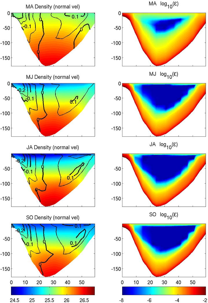
Density and mixing structure along a transect across the mouth of the Bay of Fundy (Figure 1). The left panels include density surfaces in color and normal velocity (mean Eulerian) contours for four periods: March–April, May–June, July–August and September–October. The right panels correspond to the simulated rate of turbulent dissipation (ε, Equation 1) for the same periods.

The result of the horizontal gradient in vertically-integrated mixing intensity is the presence of frontal-like structures in the density field (Figure 7, left panels) presented in simple schematic form in Figure 8. The schematic diagram is consistent with climatological fields and observed density structure from hydrographic transects during several periods (1916–1919, Mavor [1923]; 1924–1930, Hachey [1934]; 1932, Gran and Braarud [1935]; Watson [1936]; 1929–1932, Hachey and Bailey [1952]).

Figure 8.

Simple schematic of the density structure and associated circulation across the Bay of Fundy from Grand Manan Island to Nova Scotia. The vertical arrows indicate tidal mixing.

Density and normal velocity transects across the mouth of the Bay of Fundy (Figure 7, left panels) show the presence of the frontal structures in both sides of the deep basin at the center of the gyre. The isopycnals become perpendicular to the bottom at depths between 30m and 120m. In the shallower areas near both shores the water column is well-mixed. The normal velocities are calculated as the detided Eulerian mean over the last tidal cycle of the simulations. The resulting normal velocities show a shallow tidal-mixing front jet in both shores similar to the structures described in other regions (e.g., Georges Bank, Garrett and Loder [1981] and Lough and Manning [2001]; Irish Sea, Horsburgh et al. [2000]). The Grand Manan jet is more intense (∼ 0.3 ms⁻¹) than the flow near the Nova Scotia shore (∼ 0.1 ms⁻¹). The core of the jet is positioned near surface in the Grand Manan area, while in the Nova Scotia side the jet maximum varies in position from being near surface in April–May, to subsurface positions (around 50 meters) during May–June and July–August and having both a near-surface and a subsurface expression during September–October.

4.2. Potential Energy

In order to estimate the location of these frontal structures (Figure 8), several potential energy formulations are evaluated. Applications of such potential energy arguments to the Georges Bank, Gulf of Maine and Nova Scotia regions are abundant in the literature [Garrett et al., 1978; Loder and Greenberg, 1986; Perry et al., 1989; Lynch and Naimie, 1993]. First, the traditional Simpson-Hunter parameter (SH, Simpson and Hunter [1974]) is considered. A full description of this parameter can be found in Simpson [1981], but basically they assumed a balance between tidal mixing and thermal stratification. Garrett et al. [1978] evaluated this parameter for the Bay of Fundy and already discussed some limitations in the presence of fresh water runoff. The expression for the SH parameter is:

$$SH=\frac{2C_p{\epsilon }_t}{\alpha gQ}=\frac{h}{\rho C_D{u}^3}$$ (2)

where C_p is the specific heat of seawater, α is the thermal expansion coefficient, ε_t is the tidal mixing efficiency, Q is the heat flux, g is the gravitational acceleration, h is the water column depth, ρ is the density of seawater, C_D is a drag coefficient taken as 0.0027 and u is the rms size of the velocity over the period. The reference (dimensionless) value of SH used for these simulations is 10^1.9 [Garrett et al., 1978; Loder and Greenberg, 1986]. This reference value assumes tidal mixing efficiencies of ε_t = 2.6 × 10⁻³ and climatological values of heat flux during the stratified period of Q = 170W m⁻². Previous estimates by Garrett et al. [1978] were calculated from model solutions from Greenberg [1979], yet the resolution of those solutions were not sufficient to resolve the gyre and its associated potential energy balance. Lynch and Naimie [1993] presented a similar application using again just tidal solutions. The SH parameter diagnosed from the current model solutions is presented in Figure 9. Critical values represent regions where a transition from a tendency toward stratified conditions changes to a tendency toward well-mixed conditions. The critical values of the SH parameter will vary depending on the heat flux for each period. The critical value for March–April (Q = 57W m⁻²) is SH = 10^2.4. The critical value for the two summer periods, May–June (Q = 173W m⁻²) and July–August (Q = 152W m⁻²), is the reference value SH = 10^1.9. For the September–October period Q = −3.5W m⁻², suggesting there will be enough mixing everywhere in the domain to overcome stratification.

Figure 9.

Distribution of potential energy parameters [SH, Simpson and Hunter [1974]; LG, Loder and Greenberg [1986]; PE, Perry et al. [1989]] for the region around the mouth of the Bay of Fundy for four periods: (a) March–April, (b) May–June, (c) July–August, and (d) September–October. The critical SH contour is represented as a dashed gray contour. The LG critical value is marked by a black contour. The color scale represents the magnitude of the PE parameter, with zero (critical) value of PE indicated with white contours. Regions with values larger than the critical value have a tendency toward stratified conditions, while regions with parameters smaller than critical have a tendency toward well-mixed condition. In the areas where PE = PE_critical, tidal fronts are predicted. During September–October, because of the negative climatological heat flux, both the SH and LG parameters predict a tendency toward well-mixed conditions for the entire domain. In panel (d), September–October, the critical SH contour for July–August is shown for reference.

Contributions to surface energy input by wind stress are usually important, especially those by variable wind [Simpson and Bowers, 1981; Loder and Greenberg, 1986]. A modified potential energy formulation was introduced by Loder and Greenberg [1986] to account for wind mixing effects in the Gulf of Maine and Bay of Fundy:

$$LG=\frac{2C_p{\epsilon }_t^{\prime }}{\alpha gQ}=\frac{h}{D_t+\gamma \left({\epsilon }_w/{\epsilon }_t^{\prime }\right)D_w}$$ (3)

where ${\epsilon }_t^{\prime }=1.5\times {10}^{-3}$ is a reduced tidal mixing efficiency in the presence of wind mixing, $D_t=\rho C_D{u}^3$ is the same tidal current induced mixing as for SH, ε_w is the wind mixing efficiency, γ is a ratio of the transfer of energy from wind speed to wind-induced ocean speed, and D_w is the turbulent mixing due to wind. Their proposed wind mixing efficiency for this region was γ ε_w = 0.9 × 10⁻³. To consider the significant effect of the variable wind on mixing, D_w is formulated taking into account both the mean and standard deviation of the wind stress [Loder and Greenberg, 1986]. Critical values for the LG parameter during the May–June and July–August periods (Figure 9b,c) show a general tendency toward stratified conditions over the center of the Bay and a tendency toward well-mixed conditions over the shallow flanks. The LG parameter critical values (LG = 10^1.65) and distributions during the summer are consistent with the results by Loder and Greenberg [1986]. The addition of the strong mixing due to the highly variable wind stress during March–April results in a significant decrease of the extent of areas where tendencies toward stratified conditions are estimated (Figure 9a, critical SH versus critical LG).

A significant problem with the above formulations is the neglect of the freshwater contributions to buoyancy, because only heat flux contributions were considered. In the Bay of Fundy, the discharge of the St. John river, especially during spring, has a strong stratifying influence [Watson, 1936; Garrett et al., 1978; Brooks, 1994]. Several studies have established the direct effect of river discharge on potential energy by assuming a region of influence of the freshwater plume [Blanton and Atkinson, 1983; Atkinson and Blanton, 1986; Blanton et al., 1989]. This approach is useful to study the potential energy balance in the proximity of the plumes, but the effects on buoyancy over larger areas where the plume is not obvious may be neglected. To consider both the direct discharge effects on buoyancy and the modifications caused by advection of low salinity water masses from the Nova Scotian Shelf [Smith, 1983, 1989; Shore et al., 2000], we introduce the potential energy formulation used by Perry et al. [1989] for southwest Nova Scotia:

$$PE=\frac{\alpha \mathit{\text{gQh}}}{2C_p}+\frac{g{h}^3}{3\mathrm{\Delta }Z}\rho \beta \frac{\partial \mathrm{\Delta }S}{\partial t}-\left({\epsilon }_t^{\prime }{D}_t+\gamma {\epsilon }_w{D}_w\right)$$ (4)

where ΔS is the vertical change in salinity over the depth interval ΔZ, and β is the saline contraction. The critical value of PE = 0 corresponds to areas where processes that increase potential energy (usually, the first and second terms of Equation 4) balance processes that decrease potential energy (third term of Equation 4). The distribution of PE over the different periods (Figure 9) changes depending on both buoyancy (heat flux and freshwater effect on salinity) and mixing (tidal and wind) effects. During March–April (Figure 9a), tidal and variable wind mixing overcomes the buoyancy effect of the salinity difference except near the St. John river plume and close to areas affected by Scotian Shelf waters. The PE formulation may underestimate the direct effect of river discharge on buoyancy especially inside river plumes. During May–June (Figure 9b), the presence of high heat flux values and the strongest salinity stratification (as a result of the integrated effect of the spring St. John freshet) results in a strong tendency toward stratified conditions (PE >> 0) in the central part of the Bay and near the mouth of the St. John river. Over the shallow areas east of Grand Manan Island and west of Nova Scotia well-mixed conditions are expected (PE < 0). By July–August (Figure 9c), there is a decrease on the salinity-driven stratification and larger areas of the Bay tend to be well-mixed. Finally, during September–October (Figure 9d), the PE formulation suggests the presence of stratified regions that were not suggested by the formulations based only on heat flux (SH, LG). The reduced river discharge during this period results in a change to well-mixed conditions near the St. John mouth. There is a surprisingly good agreement on the location of transition areas (frontal regions) predicted with the three presented formulations (SH, LG, PE), especially from May until August.

Considering the results herein, the differential mixing mechanism for gyre intensification is only relevant during the stratified season (May–October). At these times, mixing is occurring over the shallow areas but not over the deep areas, contributing to the development of frontal structures. The secondary circulation associated with the development of tidal fronts (Figure 6) is not part of the presented potential energy models, but the presence of altered density structure associated with the fronts results in the development of cell-like structures on both sides of the frontal system [Lough and Manning, 2001; Aretxabaleta et al., 2005]. The presented potential energy formulations have several limitations (advection, direct fresh water buoyancy effects, and time evolution of these fields are assumed to be small), but the basic mechanisms are still valid as has been proven in other regions [Blanton and Atkinson, 1983; Loder and Greenberg, 1986; Perry et al., 1989; Xing and Davies, 2001].

The circulation associated with the Gyre is similar to the intensely studied flow in the Irish Sea [Hill et al., 1994; Horsburgh et al., 2000; Horsburgh and Hill, 2003]. The dynamics of the circulation associated with dense pool gyres have been described in several studies [Garrett, 1991; Hill, 1996, 1998]. The cyclonic gyre circulates around a dome of dense, usually cold, water controlled by the balance between stratification and friction, where the near-bottom density gradient drives surface flow as in other bottom-dominated fronts [Garrett and Loder, 1981; Garrett, 1991]. The dense pool circulation is present both with surface to bottom well-mixed fronts in swallow areas or just with the presence of large well-mixed bottom boundary layer. Therefore, the surface density gradient is not a needed feature of the Gyre.

4.3. Particle Retention

In order to understand the importance of the Gyre for the retention of particles, a set of numerical drifter experiments are conducted. The first experiment includes the release of fixed-depth particles in the mean May–June climatological velocity fields. The particles are released along a NW-SE line from the center of the Gyre to the Nova Scotia shelf for 30 days and follow the streamlines of the depth-averaged velocity field (Figure 10). The main characteristic observed is the circulation of particles around the center of the Gyre, with a tendency to accumulate over the deeper parts of the Gyre. Particles tend to be ejected from the Gyre at the 100m isobath south of Gran Manan Island. This first experiment considers only the mean Eulerian flow, but the general regions of accumulation and loss could be identified. The exit point location corresponds with the region of convergence at the mouth of the Bay mentioned in Section 3.1 and is located around the area surrounding the 100m isobath. Associated with the convergence in this region, downwelling is present in the simulations, with the May–June period having the strongest vertical velocities (not shown). The retention of particles in the Gyre is enhanced by this combination of convergence and downwelling. Particles released near that location at different bottom depths have a strong tendency to follow their release isobath into the Maine Coastal Current (not shown).

Figure 10.

Particles released in static mean May–June climatological depth-averaged velocity field. Particles are released every two days for 30 days along a NW-SE line (blue dots). The red dots represent the position of the particles every two days. Blue vectors represent mean depth-averaged velocities.

The retention of particles in the Gyre in the time-dependent climatological fields is studied by releasing fixed-depth particles at two depths (5m and 15m below mean sea level) from a uniform distribution with particles every 3–4 km in the entire domain and evaluating the resulting fields after 60 tidal cycles (~ 1 month). The results for the July–August period are presented in Figure 11. Most of the particles that are released in the upper Bay of Fundy get advected out of the Bay, except for the accumulation that occurs in the area inside the Gyre. There is a net increase in the concentration of particles in the central part of the Gyre, especially at 15m during July–August. Similar results are obtained for the May–June period (not shown). The regions of accumulation and loss in this Lagrangian simulation are the same as in the previous Eulerian simulation (Figure 10) suggesting the mean Gyre flow controls retention in the Bay.

Figure 11.

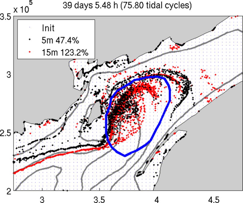
Particles released at two depths (5m and 15m below mean sea level) in a uniform distribution with particles every 3–4 km over the entire model domain during the July–August period. Particles are tracked for 60 tidal cycles and the final position is shown. The number of particles inside the blue contour are considered to be accumulated in the Gyre. Percentage change from the initial number of particles in the Gyre area is included.

In order to evaluate the retention of particles in the Gyre two more experiments are conducted: 1) with fixed-depth particles, and 2) with passive particles. A constant number of particles (∼ 20000) are released at each of three different depths (3m, 10m, and 20m below mean sea level) inside the Gyre. The averaged position of the Gyre is defined as the first closed transport streamline (0.11 Sv) of the May–June climatological simulation. Both fixed-depth and passive particles are tracked for 60 tidal cycles (∼ 1 month). The initial and final position of the fixed-depth particle experiment for the July–August period is presented in Figure 12. Most of the particles that leave the area surrounding the Gyre are lost in the initial 10–20 tidal cycles. The rest of the particles remain predominantly in the Gyre area. After 60 tidal cycles, 47.9% of the total particles released at 10m remain in the Gyre, while 60.3% of the particles released at 20m remain. The particles that are released at 3m are advected out of the Bay of Fundy area in 40 tidal cycles, so by the end of the simulation period (60 tidal cycles) there are almost no particles left (0.1%).

Figure 12.

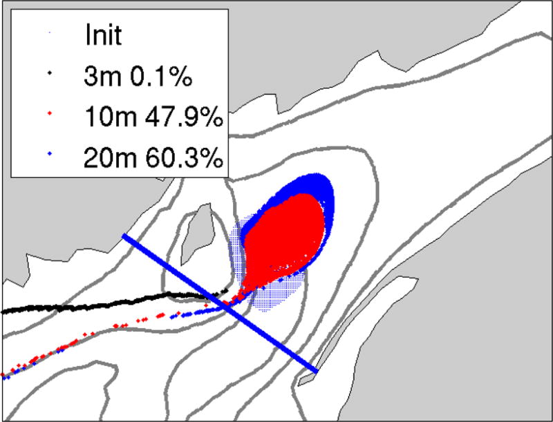
Fixed-depth particle released in July–August time-dependent 3-D climatological velocity field. Particles are released at the beginning of a 1 month simulation in a region defined by the 0.11 Sv transport streamline of the May–June climatological depth-averaged velocity at three depths: 3m, 10m, and 20m (small blue dots). The final position after 60 tidal cycles of the 3m particles are represented by black dots, the final position for 10m are represented by red dots, and the 20m ones by blue dots.

We evaluate the retention properties of the Gyre by fitting functions to the evolution of the decay in the total number of particles that remained in the Bay of Fundy (Figure 13). The proposed modified logistic curve that describes the observed distribution follows the equation:

$$P(t)=P_0+\kappa -\frac{P_0\kappa e^{\mathrm{\lambda }t}}{P_0+\kappa (e^{\mathrm{\lambda }t}-1)}$$ (5)

where P (t) is the particle concentration at any time, P₀ is the initial number of released particles, κ is number of particles remaining at t → ∞, and λ is the particle decay rate. P (t) is the solution of the differential equation:

$$\frac{d\stackrel{\sim }{P}}{dt}=\mathrm{\lambda }\left(\stackrel{\sim }{P}-{\beta }_{\infty }-1\right)\left(\stackrel{\sim }{P}-{\beta }_{\infty }\right)$$ (6)

where $\stackrel{\sim }{P}=P/P_0$ is a dimentionless particle concentration and β_∞ = κ/P₀ is the concentration at t → ∞. The appropriateness of the logistical fit is evaluated by calculating the root mean square difference (RMSE) between curve and model retention. The mean RMSE value for all cases is less than 5% of the total signal (range between 3.0% and 6.6%).

Figure 13.

Evolution of the decay in the total number of particles that remained in the Bay of Fundy for the July–August period and fit to a logistical curve. Three different depths (3, 10, and 20m) are represented by black, red, and blue lines, respectively.

The characteristic of the retention associated with the Gyre can be then simplified to two parameters: 1) λ, the particle decay rate and 2) β_∞, the concentration of particles that tend to remain in the Gyre after the period of initial decay. We calculate the half life time scale (time when the mean value between κ and P₀ is encountered), as a measure of retention times in the Gyre. The half life follows Equation 7:

$$t_{1/2}=\frac{1}{\mathrm{\lambda }}\text{log}\left(\frac{{\beta }_{\infty }+1}{{\beta }_{\infty }}\right)$$ (7)

We present the retention characteristics of the Gyre for different periods according to these two parameters (Tables 1 and 2). The main result is an increased retention during three periods (May–Jun, Jul–Aug, and Sep–Oct) with respect to the March–April period with significant amounts of particles (∼ 50%) remaining in the Gyre for long periods of time (more than 30 days) at 10m and 20m. Retention predominantly increased with depth, with small retention near the surface and both larger β_∞ and decay times in deeper layers. The surface layer (3m) is, in fact, very dispersive for all periods. The retention during the March–April period is smaller for both parameters at all depths and for both fixed-depth and passive particles. Note that β_∞ values between 2–8% are sensitive to the duration of the particle tracking experiments. If the model simulations were longer, the curve fitting would produce values of β_∞ closer to zero. Therefore, the values of β_∞ less than 10% can be considered as a tendency of the Gyre to lose all particles.

Table 1.

Retention parameters for all fixed-depth simulations using a logistical curve to fit the particle concentration decay in the Gyre (as in Figure 13). β_∞, concentration (percentage) of particles at t → ∞, and t_1/2, half life decay time (days).

	Mar–Apr		May–Jun		Jul–Aug		Sep–Oct
	β∞	t1/2	β∞	t1/2	β∞	t1/2	β∞	t1/2
3m	2%	6.3	16%	7.9	6%	6.6	10%	7.2
10m	3%	8.1	55%	5.3	43%	4.5	49%	6.4
20m	7%	10.3	52%	9.0	57%	4.2	53%	7.3

Table 2.

As in Table 1, but for passive particles. β_∞, concentration (percentage) of particles at t → ∞, and t_1/2, half life decay time (days).

	Mar–Apr		May–Jun		Jul–Aug		Sep–Oct
	β∞	t1/2	β∞	t1/2	β∞	t1/2	β∞	t1/2
3m	3%	6.5	14%	7.4	9%	6.1	11%	6.9
10m	18%	5.2	46%	6.9	34%	5.7	30%	10.9
20m	25%	4.8	43%	9.5	45%	6.2	38%	11.3

The differences in retention between fixed-depth and passive particles are that during the stratified periods (May–October) less total passive particles tend to remain in the Gyre (smaller β_∞), while their half lives are larger. During March–April, the opposite behavior is observed, with more passive than fixed-depth particles remaining, though with shorter half lives.

Several factors determine the fluctuations in the presented retention times: the strength of the flow around the Gyre (stronger between May and October), the spatial extent of the Gyre (slightly larger closed transport streamline during May–June), the level of stratification that results in a stronger velocity shear in the vertical (stronger during July–August and weaker during spring), the wind stress (stronger in March–April) and heat-flux strength (maximum in May–June), and the variability of the convergence at the entrance to the Bay between north flow from western Nova Scotia and south flow coming across the Grand Manan Island shoals. The combination of factors results in lowest retention during March–April. When the stratification starts to develop in May–June, the strength of the Gyre flow increases as well as the convergence near the mouth of the Bay, resulting in high retention. The stronger stratification in July–August, with associated stronger vertical shear and increased cross-Bay surface flow, slightly reduces the retention during that period. During September–October stronger mean winds affect the level of stratification and retention of fixed-depth particles increases slightly, while retention of passive particles is reduced. Therefore, stratification increases retention as long as it does not result in strong near-surface cross-Bay flow. The results presented are for near-surface releases, but significantly different results are obtained by releasing particles deeper in the water column (not shown).

5. Discussion

Previous studies [Dickie, 1955; Lauzier, 1967; Godin, 1968] have inferred from a few observations the possibility of counter-clockwise circulation in the region near the mouth of the Bay of Fundy. Herein we have used numerical simulations to provide a systematic description of the structure and variability of the Bay of Fundy Gyre, including the partitioning between different forcings, the articulation of an intensification mechanism, and the quantification of the retention characteristics of the Gyre.

The basic structure of the Gyre is related to the presence of strong tidal flow in the Bay of Fundy. The tidal rectification associated with the tidal motions over steep topography creates strong residual circulation in the western, eastern and to a lesser degree, the northern, sides of the deeper central basin of the lower Bay of Fundy (Figure 2b). Additionally, during periods when stratification is enhanced (i.e., spring river discharge providing increased buoyancy, spring-summer high heat flux), the balance between tidal mixing and stratification shifts, producing regions (shallow flanks) with sufficient mixing to overcome buoyancy in relatively close proximity to regions (deep basins) where stratification is maintained. This process results in tidal front-like structures (Figure 8), where the general counter-clockwise flow of the Gyre is intensified. This process was partially described by Dickie [1955] to explain the temperature variability in the region between periods of “closed” and “open” circulation. The balance between tidal mixing and stratification and its relation to frontal position in this area was first introduced by Garrett et al. [1978]. The associated circulation is consistent with flow around a cool water pool [Hill, 1998].

The main characteristics of the mean Eulerian secondary flow associated with the tidal front (Figure 6) are the presence of upwelling in the mixed region (over the shallower areas) and the occurrence of downwelling in the stratified region (deeper areas). Associated with the downwelling, there is near-surface convergence and near-bottom divergence. The combined effect of this secondary circulation is the appearance of cell-like circulation patterns. The mean (Eulerian) upwelling and downwelling exhibit high temporal and spatial variability due to the effect of the strong tidal dynamics (currents and mixing) in the region. Therefore, the synoptic residual fields could differ substantially from observed fields at any particular time. The retention of particles in the Gyre is partially controlled by the frontal structures. The secondary circulation associated with the fronts facilitates the retention of passive particles [Lough and Manning, 2001; Aretxabaleta et al., 2005] and therefore the presence of recirculation cells helps particle retention in the Gyre.

The effect of the wind stress is especially important in the March–April period, when the stronger mean wind stress causes both the removal of the surface stratification (Figure 7) and the transport of particles outside the Bay of Fundy. The limited retention in the layers closer to the surface is due to stronger wind-driven advection.

The interaction between the Bay of Fundy Gyre and the adjacent circulation of the Gulf of Maine is an additional factor controlling the fate of particles in the Bay. Convergence and downwelling in the area between the 100m and 150m isobaths associated with the interaction between the Gyre, the Maine Coastal Current and the north flow west of Nova Scotia causes fluctuations in the retentiveness of the gyre. During periods when the convergence and downwelling is more intense (May–June), the resulting retention of particles is consequently increased.

6. Conclusions

The basic mechanisms controlling the presence and variability of the Bay of Fundy Gyre have been described. Tidal rectification associated with the steep bathymetry around western Nova Scotia and Grand Manan Island, creates opposing flows on opposite sides and a weaker west flow in the north. The density structure contributes to the circulation around the Gyre by both closing the north and south edges of the Gyre and extending the region with clockwise circulation further north into the Bay. The St. John river discharge has a significant effect on surface velocity, especially during March–April, but a small effect on the depth-averaged flow. The climatological wind, especially during the summer months, has a limited effect on the intensity and overall structure of the Gyre. The effect of wind pulses and variability has been omitted from this study and will be addressed in a companion hindcast study.

Flow around the Gyre is stronger during July–August and September–October with velocities on the order of 0.05 – 0.15 ms⁻¹ (consistent with Godin [1968]) resulting from the combination of tidal rectification and baroclinic flow. The velocities during March–April are weaker due to the lack of a strong baroclinic effect. The spatial extent of the Gyre is relatively constant during the summer months, with a predicted slightly larger extent for the May–June period. The connection of the Gyre circulation with the adjacent Gulf of Maine flow seems to be an important factor in controlling the flow around the southern edge of the Gyre and the advective exchange between the two regions.

Differential tidal mixing, between the deep basin at the mouth of the Bay of Fundy and the shallow flanks around Grand Manan Island and western Nova Scotia, is the main factor controlling the Gyre intensification during the stratified season. The differential mixing creates frontal-like structures that maintain secondary circulation that have a significant contribution to the retention of particles by the Gyre. Intensive surveying, similar to studies conducted in the Irish Sea [Horsburgh et al., 2000], will be needed to corroborate the structure and variability of the Gyre.

The model simulations suggest a maximum retention during the May–June period in the depths between 10–20m from the surface with residence times longer than 30 days for around 50% of the particles released and a half life time for the particles that exited the Gyre of 5–9 days. The retention values for July–August and September–October are slightly smaller. Particles released closer to the surface have much weaker retention (2–16% of long retention and half life 6–8 days). A similar behavior is observed for the March–April period at all depths associated with weaker frontal circulation and much stronger average winds.

The biological implications of the described retention characteristics of the Gyre are significant. One current application will be to the understanding and prediction of the distribution and evolution of A. fundyense both in the Bay of Fundy and the Gulf of Maine. The retentive nature of the Gyre favors the self-sustainability of the Bay of Fundy population of this dinoflagellate and creates the possibility of the cyst bed located in the Bay acting as a long-term source for the Gulf of Maine population.

References

- Apollonio S. The Gulf of Maine, Courier-Gazzete Books. 1979:61. [Google Scholar]
- Aretxabaleta A, Manning JP, Werner FE, Smith KW, Blanton BO, Lynch DR. Data assimilative hindcast on the southern flank of Georges Bank during May 1999: Frontal circulation and implications. Cont Shelf Res. 2005;25:849–874. [Google Scholar]
- Atkinson LP, Blanton JO. Processes that affect stratification in shelf waters, in. In: Mooers CNK, editor. Baroclinic processes on Continental Shelves. American Geophysical Union; Washington, D. C.: 1986. pp. 117–130. [Google Scholar]
- Bigelow HB. Physical oceanography of the Gulf of Maine. Bull US Bur Fish. 1927;49:511–1027. [Google Scholar]
- Bigelow HB. Explorations of the waters of the Gulf of Maine. Geograph Rev. 1928;18:232–260. [Google Scholar]
- Blanton JO, Atkinson LP. Transport and fate of river discharge on the continental shelf off the southeastern United States. J Geophys Res. 1983;88:4730–4738. [Google Scholar]
- Blanton JO, Oey LY, Amft J, Lee TN. Advection of momentum and buoyancy in a coastal frontal zone. J Phys Oceanogr. 1989;19:98–115. [Google Scholar]
- Brooks DA. Vernal Circulation of the Gulf of Maine. J Geophys Res. 1985;90:4687–4705. [Google Scholar]
- Brooks DA. A model study of the buyancy-driven circulation in the Gulf of Maine. J Phys Oceanogr. 1994;24:2387–2412. [Google Scholar]
- Brooks DA, Townsend DW. Variability of the coastal current and nutrient pathways in the Gulf of Maine. J Mar Res. 1989;47:303–321. [Google Scholar]
- Brown WS, Irish JD. The annual evolution of geostrophic flow in the Gulf of Maine: 1986–1987. J Phys Oceanogr. 1992;22:445–473. [Google Scholar]
- Campbell A. Application of a yied and egg-per-recruit model to the lobster fishery in the Bay of Fundy. N Am J Fish Manag. 1985;5:91–104. [Google Scholar]
- Chao SY, Boicourt WC. Onset of estuarine plumes. J Phys Oceanogr. 1986;16:2137–2149. [Google Scholar]
- Dickie LM. Fluctuations in abundance of the giant scallop, Placopecten magellanicus (Gmelin), in the Digby Area of the Bay of Fundy. J Fish Res Bd Canada. 1955;12:797–857. [Google Scholar]
- Fish CJ, Johnson MW. The biology of the zooplankton population in the Bay of Fundy and Gulf of Maine with special reference to production and distribution. J Biol Bd Can. 1937;3:189–322. [Google Scholar]
- Garrett CJR. Tidal resonance in the Bay of Fundy and Gulf of Maine. Nature. 1972;238:441–443. [Google Scholar]
- Garrett CJR. Marginal mixing theories. Atmos-Ocean. 1991;29:313–339. [Google Scholar]
- Garrett CJR, Loder JW. Dynamical aspects of shallow sea fronts. Phil Trans R Soc Lond. 1981;302:563–581. [Google Scholar]
- Garrett CJR, Keely JR, Greenberg DA. Tidal mixing versus thermal stratification in the Bay of Fundy and Gulf of Maine. Atmos-Ocean. 1978;16:403–423. [Google Scholar]
- Godin G. Tech rep, Marine Sciences Branch, Energy Mines and Resources. Ottawa, Canada: 1968. The 1965 current survey of the Bay of Fundy: A new analysis of the data and an interpretation of results. Manuscript Rep. Ser. No. 8; p. 97. [Google Scholar]
- Gran HH, Braarud T. A quantitative study of the phytoplankton in the Bay of Fundy and the Gulf of Maine (including observations on hydrography, chemistry and turbidity) J Biol Bd Can. 1935;1:279–467. [Google Scholar]
- Greenberg DA. A numerical model investigation of tidal phenomena in the Bay of Fundy and Gulf of Maine. Marine Geodesy. 1979;2:161–187. [Google Scholar]
- Greenberg DA. Modeling the mean barotropic circulation in the Bay of Fundy and Gulf of Maine. J Phys Oceanogr. 1983;13:886–904. [Google Scholar]
- Hachey HB. The replacement of Bay of Fundy waters. J Biol Bd Can. 1934;1:121–131. [Google Scholar]
- Hachey HB, Bailey WB. Tech rep, Fish Res Bd Canada. St Andrews, N.B., Canada: 1952. The general circulation of the waters of Bay of Fundy. ms rep. biol. sta., no. 455; p. 100. [Google Scholar]
- Hannah CG, Shore J, Loder JW, Naimie CE. Seasonal circulation on the western and central Scotian Shelf. J Phys Oceanogr. 2001;31:591–615. [Google Scholar]
- He R, McGillicuddy DJ, Lynch DR, Smith KW, Stock CA, Manning JP. Data Assimilative Hindcast of the Gulf of Maine Coastal Circulation. J Geophys Res. 2005;110 [Google Scholar]
- Hill AE. Spin-down and the dynamics of dense pool gyres in shallow seas. J of Marine Research. 1996;54:471–486. [Google Scholar]
- Hill AE. Buoyancy effects in coastal and shelf seas. In: Brink KH, Robinson AR, editors. The Sea. Vol. 10. Academic Press; 1998. pp. 21–62. [Google Scholar]
- Hill AE, Durazo R, Smeed DA. Observations of a cyclonic gyre in the western Irish Sea. Cont Shelf Res. 1994;14:479–490. [Google Scholar]
- Horsburgh KJ, Hill AE. A three-dimensional model of density-driven circulation in the Irish Sea. J Phys Oceanogr. 2003;33:343–365. [Google Scholar]
- Horsburgh KJ, Hill AE, Brown J, Fernand L, Garvine RW, Angelico MMP. Seasonal evolution of the cool pool gyre in the western Irish Sea. Progr Oceanogr. 2000;46:1–58. [Google Scholar]
- Hunt JJ, Neilson JD. Is there a separate stock od Atlantic cod in the westen side of the Bay of Fundy. N Amer J Fish Man. 1993;13:421–436. [Google Scholar]
- Lauzier LM. Bottom residual drift on the Continental Shelf area of the Canadian Atlantic coast. J Fish Res Bd Canada. 1967;24:1845–1859. [Google Scholar]
- Loder JW, Greenberg DA. Predicted positions of tidal fronts in the Gulf of Maine. Cont Shelf Res. 1986;6:397–414. [Google Scholar]
- Loder JW, Shore JA, Hannah CG, Petrie BD. Decadal-scale hydrographic and circulation variability in the Scotia-Maine region. Deep-Sea Research II. 2001;48:3–35. [Google Scholar]
- Lough RG, Manning J. Tidal-front entrainment and retention of fish larvae on the southern flank of Georges Bank. Deep-Sea Research II. 2001;48:631–644. [Google Scholar]
- Lynch D, Naimie C. The M2 tide and its residual on the outer banks of the Gulf of Maine. J Phys Oceanogr. 1993;23:2222–2253. [Google Scholar]
- Lynch DR, Werner FE. Three-dimensional hydrodynamics on finite elements. Part II: Non-linear time-stepping model. Int J Numer Methods Fluids. 1991;12:507–533. [Google Scholar]
- Lynch DR, Ip JTC, Naimie CE, Werner FE. Comprehensive coastal circulation model with application to the Gulf of Maine. Cont Shelf Res. 1996;16:875–906. [Google Scholar]
- Lynch DR, Holboke MJ, Naimie CE. The Maine Coastal Current: Spring climatological circulation. Cont Shelf Res. 1997;17:605–634. [Google Scholar]
- Lynch DR, et al. Real-time data assimilative modeling on Georges Bank. Oceanography. 2001;14:65–77. [Google Scholar]
- Martin JL, White AW. Distribution and abundance of the toxic dinoflagellate Gonyaulax excavata in the Bay of Fundy. Can J Fish Aquat Sci. 1988;45:1968–1975. [Google Scholar]
- Mavor JW. The circulation of the water in the Bay of Fundy. Part I. Introduction and drift bottle experiments. Cont Can Biol. 1922;1:103–124. [Google Scholar]
- Mavor JW. The circulation of the water in the Bay of Fundy. Part II. The distribution of temperature, salinity and density in 1919 and the movements of the water which they indicate in the Bay of Fundy. Cont Can Biol. 1923;1:355–375. [Google Scholar]
- McGillicuddy DJ, Anderson DM, Lynch DR, Townsend DW. Mechanisms regulating large-scale seasonal fluctuations in Alexandrium fundyense populations in the Gulf of Maine: results from a physical-biological model. Deep-Sea Research. 2005;52:2698–2714. [Google Scholar]
- Mellor G, Yamada T. Development of a turbulence closure model for geophysical fluid problems. Rev of Geophys Space Phys. 1982;20:851–875. [Google Scholar]
- Mountain DG, Strout GA, Beardsley RC. Surface heat flux in the Gulf of Maine. Deep-Sea Research II. 1996;43:1533–1546. [Google Scholar]
- Naimie CE. Georges Bank residual circulation during weak and strong stratification periods: prognostic numerical model results. J Geophys Res. 1996;101:6469–6486. [Google Scholar]
- Naimie CE, Loder JW, Lynch DR. Seasonal variation of the three-dimensional residual circulation on Georges Bank. J Geophys Res. 1994;99:15,967–15,989. [Google Scholar]
- Perry RI, Hurley PCF, Smith PC, Koslow JA, Fournier RO. Modelling the initiation of spring phytoplankton blooms: a synthesis of physical and biological interannual variability off southwest Nova Scotia, 1983–1985. Can J Fish Aquat Sci. 1989;46(Suppl 1):183–199. [Google Scholar]
- Pettigrew NR, Townsend DW, Xue H, Wallinga JP, Brickley PJ, Hetland RD. Observations of the Eastern Maine Coastal Current and its offshore extensions. J Geophys Res. 1998;103:30,623–30,640. [Google Scholar]
- Pettigrew NR, Churchill JM, Janzen CD, Mangum LJ, Signell RP, Thomas AC, Townsend DW, Wallinga JP, Xue H. The kinematic and hydrographic structure of the Gulf of Maine Coastal Current. Deep-Sea Research II. 2005;52:2369–2391. [Google Scholar]
- Proehl J, Lynch DR, McGillicuddy D. Modeling turbulent dye transport on the northern flank of Georges Bank using Lagrangian particle methods. Cont Shelf Res. 2004;999:999–999. [Google Scholar]
- Shore JA, Hannah CG, Loder JW. Drift pathways on the western Scotian Shelf and its environs. Can J Fish Aquat Sci. 2000;57:2488–2505. [Google Scholar]
- Simpson JH. The shelf-sea fronts: Implications of their existence and behavior. Phil Trans R Soc Lond. 1981;302:531–543. [Google Scholar]
- Simpson JH, Bowers D. Models of stratification and frontal movement in shelf seas. Deep-Sea Research. 1981;28A:727–738. [Google Scholar]
- Simpson JH, Hunter JR. Fronts in the Irish Sea. Nature (London) 1974;250:404–406. [Google Scholar]
- Smith PC. The mean and seasonal circulation off southwest Nova Scotia. J Phys Oceanogr. 1983;13:1034–1054. [Google Scholar]
- Smith PC. Seasonal and interannual variability of current, temperature and salinity off southwest Nova Scotia. Can J Fish Aquat Sci. 1989;46(Suppl 1):4–20. [Google Scholar]
- Watson EE. Mixing and residual currents in the tidal waters as illustrated in the Bay of Fundy. J Biol Bd Can. 1936;2:141–208. [Google Scholar]
- White AW, Lewis CM. Resting cysts of the toxic, red tide dinoflagellate gonyaulax excavata in Bay of Fundy sediments. Can J Fish Aquat Sci. 1982;39:1185–1194. [Google Scholar]
- Xing J, Davies AM. A three-dimensional baroclinic model of the Irish Sea: Formation of the thermal fronts and associated circulation. J Phys Oceanogr. 2001;31:94–114. [Google Scholar]
- Xue H, Chai F, Pettigrew NR. A model study of the seasonal circulation of the Gulf of Maine. J Phys Oceanogr. 2000;30:1111–1135. [Google Scholar]