A marginal cure rate proportional hazards model for spatial survival data

Summary

Dental studies often produce spatially referenced multivariate time-to-event data, such as the time until tooth loss due to periodontal disease. These data are used to identify risk factors that are associated with tooth loss, and to predict outcomes for an individual patient.The rate of spatial referencing can vary with various tooth locations. In addition, these event time data are heavily censored, mostly because a certain proportion of teeth in the population are not expected to experience failure and can be considered ‘cured’. We assume a proportional hazards model with a surviving fraction to model these clustered correlated data and account for dependence between nearby teeth by using spatial frailties which are modelled as linear combinations of positive stable random effects. This model permits predictions (conditioned on spatial frailties) that account for the survival status of nearby teeth and simultaneously preserves the proportional hazards relationship marginally over the random effects for the susceptible teeth, allowing for interpretable estimates of the effects of risk factors on tooth loss. We explore the potential of this model via simulation studies and application to a real data set obtained from a private periodontal practice, and we illustrate its advantages over other competing models to identify important risk factors for tooth loss and to predict the remaining lifespan of a patient’s teeth.

1. Introduction

Periodontal disease, which contributes to eventual tooth loss, remains a major global oral health burden. Tooth loss can inflict pain and disability, and severely compromise quality of life. The Centers for Disease Control and Prevention estimates that a quarter of US adults aged 65 years or above are toothless (National Center for Chronic Disease Prevention and Health Promotion, 2011). With Americans visiting dentists 500 million times every year and the ever rising cost of medical and dental insurance premiums in the USA, development of any future dental treatment plan should seek to utilize accurate prognosis. Therefore, developing efficient statistical models to identify risk factors for tooth loss and to predict the remaining lifespan of a tooth are needed.

Consider the motivating data set of McGuire and Nunn (1996). They modelled tooth loss for 99 subjects over several years as a function of various covariates, such as baseline periodontal probing depth, defined as the distance (in millimetres) from the gingival margin to the base of the sulcus or pocket as measured by a periodontal probe. Analysing tooth loss data presents many challenges. These data exhibit spatial dependence (Banerjee et al., 2014), because tooth survival might be associated with the disease status (and survival) of a neighbouring tooth. In addition, because of diverse factors that lead to tooth loss, these data might exhibit non-stationarity, with varying patterns of spatial dependence in different regions of the mouth, as well as a complex dependence between the observations for each subject. Furthermore, tooth loss data are typically highly censored as many teeth are lost before observation begins or remain intact at the final observation. These censored survival data are also dependent within subject because of shared dietary, hygienic and other factors. From a biological perspective, many of these teeth remain sound throughout the full lifetime of a subject and can be considered non-susceptible to dental disease progression, or ‘cured’ (Sy and Taylor, 2000). Thus, the study population constitutes subjects with a mixture of both susceptible and non-susceptible teeth.

Tooth loss data have been modelled by using standard Kaplan–Meier survival analysis techniques (Chuang et al., 2001; Härkänen et al., 2002), regressions accommodating clustered interval-censored structure of the data (Wong et al., 2005), via non-spatial proportional hazard (PH) frailty models (Manda et al., 2005) and marginal models (Spiekerman and Lin, 1998; Chuang et al., 2002). Some recent advances in this direction also include the extensions of the classification and regression trees methodology to correlated survival outcomes (Fan et al., 2006, 2009).

A variety of methods have been proposed for spatially referenced survival data. From an interpretation perspective, these methods can be broadly classified as either conditional or marginal. Conditional models introduce random effects (frailties) in either the PH (Li and Ryan, 2002, Banerjee et al., 2003; Hennerfeind et al., 2006) or proportional odds (Banerjee and Dey, 2005) framework and then use Gaussian spatial models for the frailties to account for spatial dependence. These methods are referred to as conditional because the regression coefficients are interpreted conditionally on the spatial frailties. In some cases, e.g. identifying population level risk factors for tooth loss, the conditional interpretation can be awkward because the frailties are essentially nuisance parameters that are used to capture spatial dependence, and the effects of the regression parameters marginally over the frailties do not have a closed form. Li and Lin (2006) proposed a marginal model to overcome this limitation. In this model, the data are transformed to Gaussian and modelled directly (i.e. without frailties) by using a Gaussian spatial model, thus preserving the marginal interpretation of the regression coefficients. However, this model does not preserve the well-accepted PH interpretation of the regression coefficients and does not permit estimation of spatial frailties which can be used to identify at-risk regions. Further extensions to accommodate a cured proportion along with spatial dependence in survival data appear in Banerjee and Carlin (2004) and Cooner et al. (2006).

In this paper, we model tooth loss by using a mixture cure (Sy and Taylor, 2000) spatial survival model that accounts for both susceptible and non-susceptible teeth and the dependence between the event times of nearby teeth. Here, we assume that a fraction π of the entire teeth population is cured, and the remaining 1 − π remaining susceptible (non-cured). Hence, the survival function for the whole population S(t) can be written as S(t) = π + (1 − π)S₁(t), where S₁ (t) is the survival function for the non-cured teeth. Note that, under π > 0, S(t) is no longer a survival function (S(∞) = π); however, S₁(t) is. We assume a PH relationship between the covariates and the survival outcome S₁(t) for the non-cured teeth, and we use frailties to account for spatial dependence between nearby teeth. However, rather than a Gaussian model for the random effects, we model the frailties as linear combinations of positive stable (PS) random variables (Hougaard, 1986). For non-spatial data, Liu et al. (2011) showed that PS random effects preserve the PH relationship between predictors and survival marginally over the random effects. We extend this idea to the spatial setting borrowing concepts from spatial extreme value analysis (Reich and Shaby, 2012; Shaby and Reich, 2012). Note that a mixture of PH functions is no longer proportional, and S(t) does not have PH structure. Throughout the paper, our focus and model development for understanding the covariate–response relationship remains confined only to the non-cured teeth, and their survival function S₁(t). Our spatial model not only preserves the marginal PH relationship but also permits straightforward predictions of the remaining lifespan of a tooth for the non-cured teeth. In addition, the spatial dependence that is induced by this model has nice properties, including non-stationarity, and can be motivated as the limiting process under a competing risk hypothesis.

The data that are analysed in the paper and the programs that were used to analyse them can be obtained from http://wileyonlinelibrary.com/journal/rss-datasets

2. Description of the McGuire and Nunn (1996) data

The McGuire and Nunn (1996) data set consists of n=99 subjects with at least 5 years of maintenance selected from a private periodontal practice of Dr Michael K. McGuire in the Houston area. Subjects were followed for 16 years. For each tooth, the response is the time after the initial visit until tooth loss due to periodontal disease. We use p = 9 covariates. The subject level covariates are age at baseline, an indicator of poor (fair is the baseline) hygiene, an indicator of good hygiene and smoking status. The hygiene variable is an assessment of the quality of the subject’s home oral hygiene, based on looking at a patient’s plaque score, amount of calculus accumulation, bleeding index and gingival inflammation. A patient with a low plaque score, little bleeding on probing and fairly healthy gingiva would be assessed with ‘good’ hygiene. In contrast, a patient with a high plaque score, copious bleeding on probing and puffy, inflamed gingiva would be classified with ‘poor’ hygiene, with the baseline category ‘fair’ standing somewhere in between the two extremes. The binary smoking status indicated ever a smoker, or never. The baseline tooth level covariates are a crown-to-tooth ratio indicator, probing depth, mobility, an indicator of a missing adjacent tooth on the same jaw and an indicator of a missing directly opposing tooth on the opposite jaw. The crown-to-root ratio is defined as the ratio of the length of the part of a tooth that appears above the alveolar bone versus what lies below it (Penny and Kraal, 1979). Our data set records the crown-to-root ratio (binary) indicator, which is 1 if it was deemed unsatisfactory by the clinician because of periodontal disease and 0 otherwise. Mobility is defined as the amount of bone loss around the tooth and is categorized into four classes starting from complete tooth stability to a tooth being terminally mobile, i.e. bone loss of 1 mm in any direction. In our analysis, we treat it as a continuous variable.

We analyse data for m = 28 teeth for each subject (third molars are excluded). The 14 teeth on the upper jaw are numbered from 2 (left) to 15 (right), and the 14 teeth on the lower jaw are numbered from 18 (right) to 31 (left). Teeth are classified as molars (teeth 2, 3, 14, 15, 18, 19, 30 and 31), premolars (4, 5, 12, 13, 20, 21, 28 and 29), canines (6, 11, 22 and 27) and incisors (7–10 and 23–26). The spatial co-ordinates are defined as s = (s₁, s₂), where s₁ is the tooth’s right or left position (so teeth 2 and 31 have s₁ =1 and teeth 15=and 18 have s₁ =14) and s₂ as 0 for teeth on the upper jaw and 1 for teeth on the lower jaw.

We denote the event time for the tooth at location s for subject i as Y_i(s). Because the data set contains mostly subjects with well-maintained dental hygiene, the censoring rate is high. Fig. 1 presents the unadjusted Kaplan–Meier survival curves for the whole data, and stratified for the four broad tooth types: molar, premolar, canine and incisor. The survival curves level off and plateau towards the tails for all cases, thereby suggesting the possibility of the presence of a cured proportion of teeth in the data set. Averaging over subjects, 12.8% of teeth are missing before the first visit (missing), 82.8% of the teeth remain in place at the final visit (right censored) and 4.4% (122 teeth) of teeth were lost during the observation window (uncensored). The censoring indicator is δ_i(s) = 1 for teeth remaining at the final visit, and δ_i = 0 for teeth that fall out during the monitoring period. For censored observations, we denote the final observation time as Ỹ_i(s) and thus Y_i(s) ∈ (Ỹ_i(s), ∞), and we assume that a proportion π of these censored observations are cured.

Fig. 1.

Kaplan–Meier survival plots for the full McGuire and Nunn (1996) data set (———), and also stratified by the four tooth types:------, molar;······, premolar;·-·-·-, canine;– – –, incisor

3. Spatial survival model

We model Y_i(s) for locations s ∈{s₁,…, s_m} and subjects i = 1,…, n in terms of subject and tooth level covariates X_i(s) = (X_i1(s),…, X_ip(s)). We assume the PH framework for the susceptible or non-cured teeth in a mixture–cure model, and that event times are conditionally independent given spatial random effects θ_i(s) > 0. We specify the hazard function for the non-cured teeth at location s and time t > 0 as

$${\mathrm{\lambda }}_i(\mathbf{s},t)={\theta }_i(\mathbf{s})\exp \{{\mathbf{X}}_i(\mathbf{s}){\mathit{\beta }}^{\mathrm{C}}\}{\mathrm{\lambda }}_0(\mathbf{s},t),$$

where λ₀.(s, t) >0 is the baseline hazard function at location s (which is discussed further in Section 3.2). The regression coefficients, ${\mathit{\beta }}^{\mathrm{C}}={({\beta }_1^{\mathrm{C}},\dots ,{\beta }_p^{\mathrm{C}})}^{\mathrm{T}}$, are interpreted as the log-hazard-ratio conditionally (hence the superscript ‘C’) on θ. The corresponding overall survival function S(t) given the spatial frailty is

$$\mathit{P}\{{\mathit{Y}}_i(\mathbf{s})>t|{\theta }_i(\mathbf{s})\}=\pi +(1-\pi )\exp [-{\theta }_i(\mathbf{s})\exp \{{\mathbf{X}}_i(\mathbf{s}){\mathit{\beta }}^{\mathrm{C}}\}{\mathit{H}}_0(\mathbf{s},t)],$$

where ${\mathit{H}}_0(\mathbf{s},t)={\displaystyle {\int }_0^t{\mathrm{\lambda }}_0(\mathbf{s},u)}$ du is the cumulative baseline hazard and π is the proportion of the teeth not diseased, i.e. the cured proportion. For estimating the remaining lifetime of a tooth, this is the survival function of interest. Marginalizing over θ gives the population survival function

$$P\{Y_i(\mathbf{s})>t\}=\pi +(1-\pi ){\displaystyle {\int }_0^{\infty }\exp [-\theta \exp \{{\mathbf{X}}_i(\mathbf{s}){\mathit{\beta }}^{\mathrm{C}}\}{H}_0(\mathbf{s},t)]f(\theta )\mathrm{d}\theta }.$$ (1)

For studies comparing populations, this is the survival function of interest since it is the survival function of a typical subject with covariates X_i(s). However, equation (1) generally does not have a closed form or does not preserve the PH interpretation of the regression coefficients. In particular, the PH interpretation of the regression coefficients does not hold if the spatial random effects are Gaussian.

To preserve the PH interpretation while accounting for spatial dependence, the random effects are modelled by using PS random variables. We assume that the random effect is a linear combination of L PS random variables,

$${\theta }_i(\mathbf{s})={\displaystyle \sum _{l=1}^L{w}_l{(\mathbf{s})}^{1/\alpha }{A}_{il}}{A}_{il}\stackrel{\mathrm{IID}}{\sim }\mathrm{PS}(\alpha ),$$ (2)

where w_l(s) ⩾ 0 are basis functions, A_il ⩾ 0 are the corresponding coefficients and α ∈ (0, 1] controls the shape and scale of the PS distribution. Selection of L is discussed in Section 5. The kernel coefficients A_il follow the PS distribution with Laplace transformation

$${\displaystyle {\int }_0^{\infty }\exp (-At)f(A|\alpha )\mathrm{d}A}=\exp (-t^{\alpha })$$

and density f(A|α), which we denote A_il ∼ PS(α). f(A|α) does not have a closed form (Stephenson, 2009), but it can be written as

$$f(A|\alpha )={\displaystyle {\int }_0^1\frac{\alpha A^{-1/(1-\alpha )}}{1-\alpha }}c(B)\exp \{-c(B)A^{-\alpha /(1-\alpha )}\}\mathrm{d}B,$$ (3)

where

$$c(B)={\frac{\sin (\alpha \pi B)}{\sin (\pi B)}}^{1/(1-\alpha )}\frac{\sin \{(1-\alpha )\pi B\}}{\sin (\alpha \pi B)}.$$

If α = 1, f(A|α) is the point mass distribution degenerate at A = 1, the random effects are irrelevant and there is no attenuation; as α decreases towards 0, f(A|α) becomes right skewed with spatial random-effect variance tending towards ∞ and there is substantial attenuation. The basis functions determine the form of spatial dependence, as discussed further in Section 3.1. To fix the scale of the random effects, we restrict ${\displaystyle {\sum }_{l=1}^L{w}_l(\mathbf{s})}=1$ for all s.

Marginally over the spatial random effects, the survival function and corresponding hazard function become (Appendix A.1)

$$\begin{array}{c}P\{Y_i(\mathbf{s})>t\}=\pi +(1-\pi )\exp [-\exp \{{\mathbf{X}}_i(\mathbf{s}){\mathit{\beta }}^{\mathrm{M}}\}{H}_0{(\mathbf{s},t)}^{\alpha }],\\ {\mathrm{\lambda }}_i(\mathbf{s},t)=\exp \{{\mathbf{X}}_i(\mathbf{s}){\mathit{\beta }}^{\mathrm{M}}\}\alpha H_0{(\mathbf{s},t)}^{\alpha -1}{\mathrm{\lambda }}_0(\mathbf{s},t),\end{array}$$ (4)

which for the non-cured teeth correspond to a PH model with marginal (hence the superscript ‘M’) log-hazard-ratio coefficients ${\mathit{\beta }}^{\mathrm{M}}={({\beta }_1^{\mathrm{M}},\dots ,{\beta }_p^{\mathrm{M}})}^{\mathrm{T}}={(\alpha {\beta }_1^{\mathrm{C}},\dots ,\alpha {\beta }_p^{\mathrm{C}})}^{\mathrm{T}}$ and cumulative baseline hazard H₀(s, t)^α. Comparing β^C and β^M, we observe that α controls the attenuation due to spatial dependence. Note that α is both the spatial dependence parameter and the attenuation parameter, thus playing a dual role of both determining the degree of spatial dependence and conditional or marginal attenuation.

3.1. Spatial dependence

In addition to the appealing marginal interpretation of the hazard ratio parameters for the susceptible tooth, this model also provides a nice interpretation of the spatial dependence as quantified by the joint survival function for two locations s_j and s_k. To separate spatial variation in the marginal survival function from within-subject dependence, we present the joint survival probability assuming non-cure, as well as the same covariates and cumulative baseline hazard for all sites, i.e. X_i(s) = X_i and H₀(s, t) = H₀(t) for all s. Then, Appendix A.2 shows that

$$P\{Y_i({\mathbf{s}}_j)>t,Y_i({\mathbf{s}}_k)>t\}=\exp \left[-\exp ({\mathbf{X}}_i{\mathit{\beta }}^{\mathrm{M}})H_0{(t)}^{\alpha }{\displaystyle \sum _{l=1}^L{\{w_l{({\mathbf{s}}_j)}^{1/\alpha }+w_l{({\mathbf{s}}_k)}^{1/\alpha }\}}^{\alpha }}\right].$$ (5)

Borrowing a concept from extreme value analysis (Coles, 2001), we summarize joint survival by using the extremal coefficient (with a slight abuse of notation, since the spatial extremal coefficient is usually defined in terms of the joint distribution function rather than the joint survival function) ϑ(s_j, s_k) ∈ [1, 2], defined via the equation

$$P\{Y_i({\mathbf{s}}_j)>t,Y_i({\mathbf{s}}_k)>t\}=P{\{Y_i({\mathbf{s}}_j)>t\}}^{\vartheta ({\mathbf{s}}_j,{\mathbf{s}}_k)}.$$

The extremal coefficient ranges from ϑ(s_j, s_k) = 1 if Y_i(s_j) and Y_i(s_k) are completely dependent, to ϑ(s_j, s_k) = 2 if Y_i(s_j) and Y_i(s_k) are independent. From equation (5), for the PS frailty model

$$\vartheta ({\mathbf{s}}_j,{\mathbf{s}}_k)={\displaystyle \sum _{l=1}^L{\{w_l{({\mathbf{s}}_j)}^{1/\alpha }+w_l{({\mathbf{s}}_k)}^{1/\alpha }\}}^{\alpha }}.$$

Note that ϑ(s_j, s_k) holds simultaneously for all t. In our current formulation, the degree of spatial dependence remains constant over time, which is not generally so for other frailty distributions. Certainly, the degree of spatial dependence could vary with time. In comparison with the other alternatives such as the Gaussian model (which implicitly assumes asymptotic independence) and an independence model (no spatial dependence whatsoever), our balanced model seems to be a better default choice. Further comparisons between these assumptions appear in Sections 5 and 6.

There are several potential choices for the basis functions w_l(s). To satisfy the constraints that w_l(s) ⩾ 0 and ${\displaystyle {\sum }_{l=1}^L{w}_l(\mathbf{s})}=1$ for all s, we take $w_l(\mathbf{s})=\exp \{K_l(\mathbf{s})\}/{\displaystyle {\sum }_{j=1}^L\exp }\{K_j(\mathbf{s})\}$ for K_l(s) ∈ ℛ. For extreme value analysis, Reich and Shaby (2012) and Shaby and Reich (2012) used the simple model K_l(s)=−ρ(s−v_l)², where v₁,…,v_L are fixed knots and ρ>0 controls the range of spatial dependence. However, this model may not be sufficiently rich to capture the complex dependence of periodontal data which display dependence not only between nearby teeth, but also between teeth in different quadrants.

To provide a flexible model for the spatial dependence function, we use Gaussian process priors for the K_l(s) with mean E[K_l(s)]=μ, variance V{K_l(s)}= σ² and anisotropic spatial correlation corr {K_l(s_j), K_l(s_k)}=exp(−d_jk), where

$$d_{jk}={\{{(s_{j1}-s_{k1})}^2/{\rho }_1^2+{(s_{j2}-s_{k2})}^2/{\rho }_2^2\}}^{1/2}.$$ (6)

We denote this model as K_l(s) ∼^IID GP(μ, σ, ρ). Note that these L functions that constitute the basis function w_l(s) are not identical, but exchangeable, drawn from the same prior distribution which does not depend on l, leading to different posteriors as determined by the data. The model for expression (2) thus resembles the spatial factor model of Lopes et al. (2008) (without the time dimension).

We must consider identifiability carefully. Since adding a constant to each K_l will not affect the function w_l, we fix μ=0. In addition, changing the labels of the basis functions, e.g. exchanging K₁ and K₂, does not affect the likelihood. A common approach in factor analysis is to fix several elements to 0 so that the remaining elements are identified. To avoid selecting the elements to fix to 0, we elect not to constrain the K_l. Therefore, the K_l are not individually identified, which must be accounted for when monitoring Markov chain Monte Carlo convergence. Fortunately, the parameters of interest such as θ_i(s) and ϑ(s_j, s_k) are identified, and these parameters are used to assess convergence.

3.2. The baseline hazard function

The marginal and conditional survival distributions simplify in the special case of the parametric Weibull baseline hazard ${\mathrm{\lambda }}_0(\mathbf{s},t)={\kappa }^{\mathrm{C}}(\mathbf{s})\eta {(\mathbf{s})}^{-{\kappa }^{\mathrm{C}}(\mathbf{s})}{t}^{{\kappa }^{\mathrm{C}}(\mathbf{s})-1}$, with spatially varying shape κ^C(s) > 0 and scale η(s) > 0. In this parametric model, not only is the PH assumption preserved marginally; the Weibull distribution is preserved as well. The conditional and marginal distributions for non-cured teeth are

$$\begin{array}{c}{\mathit{Y}}_i(\mathbf{s})|{\theta }_i(\mathbf{s})\stackrel{\text{indep}}{~}\text{Weibull}\left({\kappa }^{\mathrm{C}}(\mathbf{s}),\exp \left[-\frac{\log \{{\theta }_i(\mathbf{s})\}+{\mathbf{X}}_i(s){\mathit{\beta }}^{\mathrm{C}}}{{\kappa }^{\mathrm{C}}(\mathbf{s})}\right]\eta (\mathbf{s})\right),\\ {\mathit{Y}}_i(\mathbf{s})~\text{Weibull}\left[{\kappa }^{\mathrm{M}}(\mathbf{s}),\exp \left\{-\frac{{\mathbf{X}}_i(s){\mathit{\beta }}^{\mathrm{M}}}{{\kappa }^{\mathbf{M}}(\mathbf{s})}\right\}\eta (\mathbf{s})\right],\end{array}$$ (7)

where κ^M(s) = α κ^C(s) is the marginal shape parameter. The survival times are independent conditionally on θ_i(s), and spatially dependent marginally with the Weibull marginal distributions at each s. In our analysis in Section 5, we assume that the Weibull shape parameter is constant throughout the mouth (κ^C(s) ≡ κ^C), and that the Weibull scale parameter varies by tooth type, with η(s) = η₁ for molars, η(s)=η₂ for premolars, η(s)=η₃ for canines and η(s)=η₄ for incisors.

The Weibull baseline hazard can also be motivated by using asymptotic arguments. Appendix A.3 shows that this spatial process is minimum stable assuming a Weibull baseline hazard with spatially constant shape κ^C(s) ≡ κ^C, i.e. define $\stackrel{\sim }{Z}(\mathbf{s})=a(N)+b(N)$ min {Z₁(s),…, Z_N(s)} as the scaled (by some a(N) and b(N) so that $\stackrel{\sim }{Z}(\mathbf{s})$ is non-degenerate) pointwise minimum of the independent and identically distributed spatial processes Z_l(s) > 0. Then, for the large class of survival functions in the Weibull domain of attraction for Z(s), the survival function of $\stackrel{\sim }{Z}(\mathbf{s})$ converges to expression (4) as N → ∞. This motivates the use of the proposed spatial survival model in cases where the events can be thought of as the result of several competing risks, and the event time is the first of the failure times corresponding to each risk.

4. Computing details

Assuming the parametric model (7), the likelihood is simply

$${\displaystyle \prod _{i=1}^N{\displaystyle \prod _{j=1}^m({\delta }_i({\mathbf{s}}_j)\pi +(1-\pi ){[1-{\mathit{F}}_{ij}^{\mathrm{C}}\{{\mathit{L}}_i({\mathbf{s}}_j)\}]}^{{\delta }_i({\mathbf{s}}_j)}{f}_{ij}^{\mathrm{C}}{\{Y_i({\mathbf{s}}_j)\}}^{1-{\delta }_i({\mathbf{s}}_j)})}},$$ (8)

where $F_{ij}^{\mathrm{C}}(y)$ is the Weibull cumulative distribution function with parameters given in model (7) for subject i at location s_j and $f_{ij}^{\mathrm{C}}(y)$ is the corresponding density function. As stated earlier, the PS density defined in equation (3) does not have a closed form. Hence, for computing, we approximate this as a Gaussian quadrature over 100 equally spaced points covering the unit interval. Further sensitivity analysis revealed that increasing the number of quadrature points increased only the computing time without any noticeable change in the posterior parameter estimates.

Because of the mixture component in the likelihood (8), none of the parameters can be factored out. Therefore, we use a Metropolis-within-Gibbs algorithm (Tierney, 1994) in R (R Core Team, 2012) for all parameters. We use log-normal candidates for parameters with positive support, logit–normal candidates for parameters in [0, 1] and Gaussian candidate distributions for parameters with support on the entire real line, with the acceptance rates tuned between 0.3 and 0.6. Details on the posterior densities of the parameters are presented in Appendix A.4. We sample two chains with widely dispersed starting values for 250000 iterations with a spacing of 5, leaving 50000 samples from each chain. Of these 50000, the first 40000 are discarded as burn-in, leaving B =10000 samples from each chain and a total of 20000 samples for computing the posteriors. Convergence is monitored by using trace plots, auto-correlation plots and the Gelman–Rubin potential scale reduction factor $\widehat{\mathit{R}}$ (Gelman and Rubin, 1992) combining the two chains, separately for all the model parameters. The $\widehat{\mathit{R}}$ -statistics for most parameters were between 1.0 and 1.2, with the exception of β for mobility and crown-to-root ratio having an $\widehat{\mathit{R}}$ of approximately 1.3. The consistent batch means estimates of Monte Carlo standard errors (Flegal et al., 2008) for all parameters ranged between 0.003 and 0.2.

Samples from the posterior predictive distribution for censored observations are immediately available from Markov chain Monte Carlo output. Predictions for censored Y_i(s) are made at each iteration by sampling from the mixture of the conditional Weibull function in expression (7) restricted to $({\stackrel{\sim }{Y}}_i(\mathbf{s}),\infty )$ and the degenerate distribution at ∞ for the cured proportion. Denoting Y_i(s)^(b) as the sample for iterations b = 1,…, B in which the predictions were finite, the posterior predictive mean for diseased teeth is approximated as ${\displaystyle {\sum }_{b=1}^B{Y}_i{(\mathbf{s})}^{(b)}/B}$, and the T-year survival probability for diseased teeth is approximated as ${\displaystyle {\sum }_{b=1}^{B}I\{Y_i{(\mathbf{s})}^{(b)}>u_i+T\}/B}$. The T -year survival probability for all teeth is approximated as

$$\pi +(1-\pi ){\displaystyle \sum _{b=1}^B\mathit{I}\{Y_i{(\mathbf{s})}^{(b)}>u_i+T\}/B.}$$

We conduct model comparison via the log-pseudomaximum likelihood (Geisser and Eddy, 1979) statistic LPML. LPML is a summary of leave-one-out cross-validation using the log-likelihood as the objective function, i.e. LPML = Σ_ij l_i(s_j), where l_i(s_j) is the conditional predictive ordinate of the observation at location s_j for subject i, given all other observations and marginalizing over all model parameters. Despite this interpretation in terms of cross-validation, LPML can be computed with a single application of the Markov chain Monte Carlo algorithm to the complete data set as shown in Gelfand and Dey (1994). Models with larger LPML are preferred.

5. Analysis of the McGuire and Nunn (1996) data

We fit cure and non-cure versions of the PS model with L = 5, 10, 15, 20, 28 factors, the model with log-Gaussian processes for the spatial frailties, i.e. log{θ_i(s) ~^IID GP(0, σ, ρ), and the independence (non-spatial) frailty model with log{θ_i(s)}~^IID PS(α)}. For identifiability, σ² (the variance parameter for the Gaussian process governing K_l(·)), ρ₁ and ρ₂ (the scale parameters in equation (6)) were all fixed to 1. For all models, we select non-informative priors ${\beta }_j^{\mathrm{C}}$, log(η_j), log(κ^C) ∼^IID N(0, variance =10²), logit(α)∼ N(0, 1) and π ∼ uniform(0, 1). Model comparison using LPML-statistics is presented in Table 1. We select the PS cure frailty model with L = 20<M factors as the best model (the largest LPML in Table 1).

Table 1.

LPML-values for various choices of PS models (varying with L), the Gaussian and the independence model with and without cure proportions

	LPML-values for the following models:
	L = 5	L = 10	L = 15	L = 20	L = 28	Gaussian	Independence
Cure	−536	−530	−485	−383	−437	−594	−648
Non-cure	–519	–511	–499	–506	–497	–524	–654

In our analysis, we assumed a parametric Weibull baseline hazard function. To evaluate the validity of this assumption, we compute the probability inverse transform statistics PIT_ij. Let F_ij(y) be the cumulative distribution functions for the marginal Weibull distribution in expression (7) for subject i at location s_j. The statistic is defined as PIT_ij = (1 − π)F_ij Y_i(s_j) for uncensored observations. For censored observations, PIT_ij is drawn uniformly from (1 − π)F_ij{Ỹ_i(s_j)} to 1, where Ỹ_i(s_j) is the final observation time. Assuming that the model fits well, PIT_ij should follow the uniform(0,1) distribution. Fig. 2 shows quantile–quantile (Q–Q-)plots of PIT_ij versus the uniform(0,1) distribution. The Q–Q-plot is computed 10 times by using different random uniform samples for censored observations. On the basis of these diagnostics, we do not suspect any glaring departures from the Weibull assumption, and we therefore proceed with this parametric analysis.

Fig. 2.

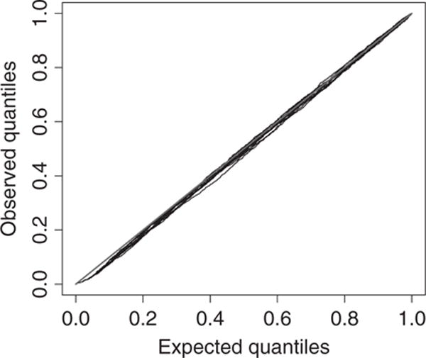
PIT_ij-diagnostic for the final PS frailties model: /, 45° line;/, observed versus expected quantiles for 10 random draws of probabilities for censored observations

Table 2 summarizes the parameters (both conditional and marginal) in the final model (the PS cure model with L = 20) and also compares the (conditional) posterior estimates from the Gaussian and the independence model. Note that these estimates can be interpreted for the susceptible (non-cured) teeth. The posterior mean (and 90% interval in parentheses) of the spatial dependence parameter α is 0.11 (0.08, 0.14), indicating strong spatial dependence, in comparison with a moderate spatial dependence (0.29 (0.23, 0.40)) for the best-fitting non-cure model (with L = 28). Note that α = 1 implies independence. Both the conditional and the marginal hazard increases for smokers and subjects with poor hygiene across all models. The spatial predictors crown-to-root ratio, probing depth and mobility all have strong positive effects on the hazard function. Interestingly, after accounting for the other predictors, there is no significant effect of missing opposite teeth at baseline; however, a missing adjacent tooth significantly increases the hazard. Note that, factoring in the cured proportion, the conditional hazards are larger for the PS model (for most parameters), compared with the Gaussian and independence models. The estimate of the Weibull shape parameter implies an increasing failure rate with time, and the survival distribution less skewed than the exponential, across all models. The scale is the smallest for molars, followed by premolars, and largest for the canines and incisors also across all models. The estimates of the cure proportion π is 0.15 (0.07,0.25) for the PS model and increases to 0.26 (0.12,0.40) for the Gaussian, and to 0.53 (0.32,0.69) for the independence model.

Table 2.

Posterior mean and 90% credible intervals of log-hazard-ratio parameters β, the Weibull shape κ and scale η, PS spatial dependence parameter α and cured proportion π

Parameter	Estimates for the following models:
	PS conditional	PS marginal	Gaussian conditional	Independence conditional
smoking status	7.02 (2.42, 11.52)	0.77 (0.27, 1.27)	1.06 (0.69, 1.43)	0.81 (0.23, 1.41)
age	–0.02 (–0.12,0.78)	–0.00 (–0.01,0.01)	–0.01 (–0.03, 0.00)	0.00 (–0.04, 0.03)
poor hygiene	8.60 (2.79, 14.26)	0.95 (0.31, 1.57)	1.16 (0.76, 1.56)	1.43 (0.82,2.06)
good hygiene	–2.00 (–7.28,3.10)	–0.22 (–0.80, 0.34)	–0.43 (–0.92, 0.04)	–0.61 (–1.26, 0.02)
crown-to-root ratio	10.36 (5.14, 15.72)	1.14(0.57, 1.73)	1.47(1.09, 1.87)	1.87 (1.34, 2.4)
probing depth	1.43 (0.63,2.18)	0.16(0.07, 0.24)	0.23 (0.13,0.33)	0.45 (0.28, 0.62)
mobility	6.40 (4.38, 8.83)	0.70 (0.48, 0.97)	0.77 (0.56, 0.97)	0.94(0.67, 1.21)
missing adjacent tooth	5.93 (3.09, 8.72)	0.65 (0.34, 0.96)	0.55 (0.15,0.96)	1.06 (0.46, 1.68)
missing opposite tooth	–1.72 (–3.86, 1.87)	–0.13 (–0.42, 0.21)	–0.15 (–0.64, 0.32)	0.40 (–0.28, 1.04)
Shape	15.34 (11.18, 19.45)	1.69(1.23,2.14)	1.87 (1.68,2.07)	2.60 (2.16, 3.13)
		PS	Gaussian	Independence
Scale, molar	—	135 (90, 202)	119(57,213)	1135 (339, 2536)
Scale, premolar	—	209 (138,314)	180 (90,316)	1375 (422, 3018)
Scale, canine	—	313 (198,439)	267 (127, 472)	1644 (492, 3665)
Scale, incisor	—	269 (186, 363)	246 (119, 435)	1599 (481,3516)
Positive stable	—	0.11 (0.08,0.14)	—	0.3 (0.3, 0.3)
Cured proportion	—	0.15 (0.07, 0.25)	0.26 (0.12, 0.40)	0.53 (0.32, 0.69)

The posterior mean of the extremal coefficient ϑ(s_j, s_k) in Fig. 3 reveals a complex non-stationary dependence for the cure and non-cure models. From Fig. 3(a) (the plot from the best-fitting non-cure model), the cluster of teeth with the strongest dependence (smallest extremal coefficient) are the anterior teeth 6–11 and 22–27. These are the incisors and canines on the upper and lower jaws respectively. Therefore, all the teeth in the front of the mouth form a cluster with strong interdependence. There is also dependence between neighbouring molars and premolars, with less dependence across quadrants for these teeth in the back of the mouth. However, Fig. 3(b) (the plot from the best-fitting cure model) presents a much smoother plot, although the degree of the overall spatial dependence is stronger than for the non-cure model. The dependence between these anterior teeth is now lower across all quadrants, with regions of strong dependence appearing spuriously. The strong spatial interdependence in Fig. 3(a) can result from groups of proximal cured (non-susceptible) anterior teeth across the subjects. Once these are not considered in the cure model, the degree of spatial interdependence between the anterior teeth overall reduces substantially (Fig. 3(b)).

Fig. 3.

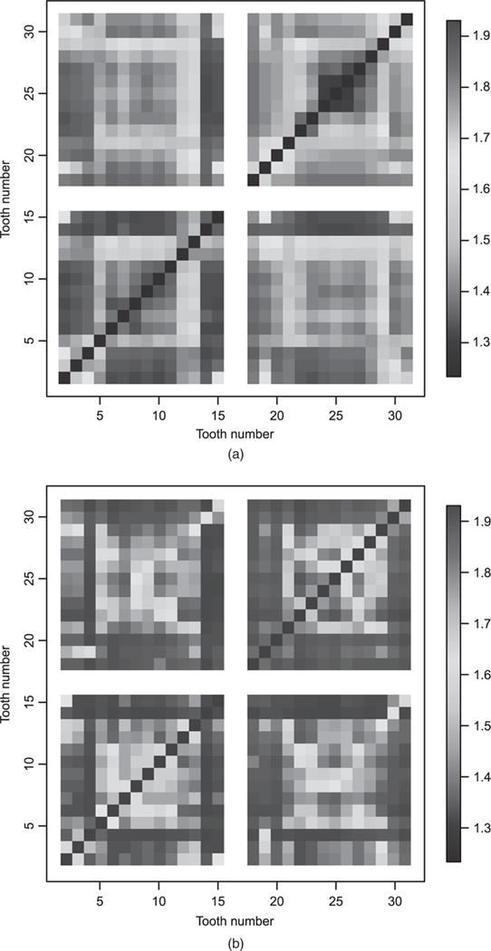
Posterior mean of the extremal coefficient ϑ(s_j, s_k) for all teeth pairs (the posterior standard deviations are all less than 0.1): (a) best-fitting PS non-cure model; (b) best fitting PS cure model

Fig. 4 summarizes the posterior predictive model for a relatively healthy subject with three teeth failures during the study, and one tooth already missing at baseline. The mean residual life (MRL) (which is defined as the expected number of additional years past the last visit until the tooth falls out) estimates for the PS model are a little higher than for the Gaussian model. Both spatial dependence and the covariates clearly affect predictions. The teeth near those that fell out during the monitoring period experience the smallest MRL, and teeth on the opposite side of the jaw also have low MRL. Teeth with large probing depth and non-zero mobility also have smaller predicted MRLs. Perhaps more relevant in practice than predictive MRLs are the posterior 5- and 10-year survival probabilities. Teeth 12 and 14, the premolar and molar in the upper jaw, have the lowest probability of surviving 5 and 10 additional years beyond the final visit. These teeth have neighbours that have fallen out, non-zero mobility and a probing depth of at least 7 mm. Their probabilities of surviving an additional 5 years are around 0.6, and their probabilities of surviving an additional 10 years are around 0.4.

Fig. 4.

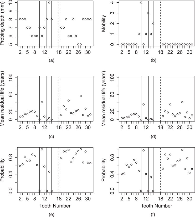
Covariates (a) probing depth and (b) mobility, (c) posterior mean residual life from the PS model, (d) posterior mean residual life from the Gaussian model, and (e) 5-year and (f) 10-year survival probabilities from the PS model for a subject with poor oral health (means are thresholded at 100 years):|, teeth missing at baseline;|, teeth that fell out during the monitoring period

6. Simulation study

In this section, we compare the finite sample performance of the regression parameter estimates for the spatial survival models with the PS, Gaussian and independence random effects. We generate data from the cure rate model for 50 subjects on a 5×2 rectangular grid with grid spacing 1, and cure fraction 0.15 (approximately representing the data). We use p = 4 covariates, with the first two X_ij(s) ≡ Xij ∼ N(0, 1) (representing subject level), and the next two X_ij(s) ∼^IID N(0, 1) (representing tooth level). The corresponding regression coefficients are β^C = (0.0, 5, 0.0, 0.5).

The baseline hazard is Weibull with shape and scale parameter constant across sites and subjects and fixed at η =2 and κ=3. Data are right censored above a threshold which is chosen as the (1 − τ)-quantile of the sample survival times, such that 100τ% of the observations are censored. Spatial random effects are simulated following either the PS or the Gaussian model. For the PS models, we choose L = 20 and use bandwidth ρ = 1. For log-Gaussian random effects, we set the variance to σ² = 0.1² and the spatial range to ρ = 1. Designs vary according to the random-effect distribution (PS or Gaussian), the strength of spatial dependence (α) and the censoring rate τ. This leads to four designs representing various data generation schemes (designs 1, 2, 3 and 4 respectively):

1. PS—weak dependence, PS random effects with α = 0.7 and τ = 0.3;

2. PS—strong dependence, PS random effects with α = 0.3 and τ = 0.3;

3. Gaussian, Gaussian random effects with τ = 0.3;

4. PS—weak with higher censoring, PS random effects with α = 0.7 and τ = 0.45.

We generate 100 data sets for each simulation design and fit the PS, Gaussian and independence models with the same priors as for the McGuire and Nunn (1996) data analysis. We compare models via the mean-squared error (MSE), bias and 90% coverage probability CP for the conditional regression coefficients β^C. Considering our parameter space β^C = (β₁, β₂, β₃, β₄) with β_j being an element of β^C and ${\widehat{\beta }}_{ij}$ the posterior estimate of β_j from the ith data set, we calculate the respective quantities as $\mathrm{MSE}({\widehat{\beta }}_j)=(1/100){{\displaystyle {\sum }_{i=1}^{100}({\widehat{\beta }}_{ij}-{\beta }_j)}}^2$, $\text{Bias}({\widehat{\beta }}_j)=(1/100){\displaystyle {\sum }_{i=1}^{100}({\widehat{\beta }}_{ij}-{\beta }_j)}$ and $\mathrm{CP}({\widehat{\beta }}_j)=(1/100){\displaystyle {\sum }_{i=1}^{100}I({\beta }_j\in [{\widehat{\beta }}_{ij,\mathrm{LCL}},{\widehat{\beta }}_{ij,\mathrm{UCL}}])}$, where I is an indicator function for β_j lying in the interval $[{\widehat{\beta }}_{ij,\mathrm{LCL}},{\widehat{\beta }}_{ij,\mathrm{UCL}}]$ with ${\widehat{\beta }}_{ij,\mathrm{LCL}}$ and ${\widehat{\beta }}_{ij,\mathrm{UCL}}$ the estimated lower and upper end points of the 90% credible intervals respectively of β_j for the ith data set. Table 3 presents these estimates for each design and covariate.

Table 3.

MSE, bias and 90% coverage probabilities for estimating conditional regression coefficients from the simulation study

Design	Model	Results for the following parameters:
		β1 = 0	β2 = 0.5	β3 = 0	β4 = 0.5
(a) MSE (× 100)
1, PS—weak	PS	2.00	2.50	0.78	1.32
	Gaussian	1.09	3.55	0.47	2.97
	Independence	1.88	2.83	0.76	1.77
2, PS—strong	PS	11.92	12.19	0.87	1.69
	Gaussian	1.18	15.76	0.35	12.52
	Independence	2.21	11.40	0.56	11.29
3, Gaussian	PS	1.89	38.10	1.29	43.93
	Gaussian	0.59	0.64	0.41	0.47
	Independence	0.98	1.80	0.72	1.81
4, PS—higher censoring	PS	2.63	3.73	1.10	2.50
	Gaussian	0.96	3.52	0.66	2.31
	Independence	1.70	3.08	1.05	1.59
(b) Bias (× 100)
1, PS—weak	PS	1.48	5.77	0.08	4.49
	Gaussian	1.33	−15.89	0.40	−15.86
	Independence	1.87	−9.89	0.91	−9.32
2, PS—strong	PS	−1.26	13.15	0.19	7.59
	Gaussian	−0.71	−32.9	0.56	−34.69
	Independence	−0.06	−30.17	1.11	−32.36
3, Gaussian	PS	1.09	28.77	−0.15	29.63
	Gaussian	0.53	−1.18	−0.11	−1.49
	Independence	0.01	8.07	−0.44	8.39
4, PS—higher censoring	PS	0.46	8.59	0.28	9.63
	Gaussian	0.02	−13.95	0.91	12.28
	Independence	0.28	−8.12	0.62	−6.35
(c) Coverage probability of 90% intervals (× 100)
1, PS—weak	PS	88	90	90	87
	Gaussian	69	33	89	19
	Independence	62	51	79	61
2, PS—strong	PS	90	86	92	85
	Gaussian	68	4	92	0
	Independence	58	11	91	1
3, Gaussian	PS	87	63	88	60
	Gaussian	85	85	91	86
	Independence	74	62	81	64
4, PS—higher censoring	PS	91	90	91	81
	Gaussian	84	47	81	49
	Independence	67	60	74	70

From the MSE values, it is clear that, even when the true model is PS with low censoring (designs 1 and 2), the parameters representing the null effect (β₁ = β₃ = 0) have higher MSE for the PS compared with the Gaussian and independence models. However, for non-null β (β₂ = β₄ = 0.5), PS enjoys lower MSE mostly. When the true model is Gaussian, the differences in MSEs between the PS and Gaussian models are much higher for the non-null β compared with the null β. Under design 4 (PS truth with moderately heavy censoring), the performance of the Gaussian model is somewhat better for the null parameters and slightly better for the non-null parameters with respect to the MSE. Interestingly, the independence model enjoys lower MSE compared with the PS model. Under designs 1 and 2, there is substantial bias under the Gaussian and independence models compared with the PS model for non-null β. Similarly, under a Gaussian true model, the bias is considerable for the PS model with respect to non-null β. Under design 4, the bias is higher for the Gaussian model for non-null β. Once again, under designs 1 and 2, the Gaussian and independence models exhibit substantial undercoverage across all parameters (except the tooth level null β₃), with the performance worsening for non-null β under design 2. Under Gaussian truth, both the PS and the independence models exhibit undercoverage for the non-null β₂ and β₄. Overall, the non-null effects are estimated more precisely by the true model. Surprisingly, this is not so for the estimation of null effects mainly with respect to MSE and bias.

As pointed out by the Associate Editor, there are some very large MSEs or biases and very poor coverages for the estimation of non-null effects in misspecified models under designs 2 and 3. In particular, all three models perform poorly in terms of MSE, with the magnitude considerably higher (43.93) for the PS model under a Gaussian true model compared with the Gaussian and independence model under PS strong truth. However, the biases are comparable in magnitude but with opposite signs, implying overestimation by the PS model and underestimation by the Gaussian and independence models. From these, we observe that the variances of the PS estimates, overall, might be larger under misspecification. This can be partly explained by the heavier tails in the PS density compared with the Gaussian or the independence (Nolan, 2015) models. The underestimation in the Gaussian and independence models is also reflected in the extremely poor CPs, whereas the CPs for the PS model under a Gaussian true model are not that poor. This rekindles our enthusiasm for the PS option. We cautiously summarize that estimation of conditional effects is highly sensitive to the underlying random-effects distribution. In general, conditional effects are less robust compared with marginal effects (Boehm et al., 2013), which is intuitive since more information is available for estimating marginal effects than conditional effects.

7. Conclusion

In this paper, we propose a mixture cure PH model for spatially referenced survival data under a Bayesian paradigm. Our model induces spatial dependence via random effects and preserves the PH interpretation of the covariates (for the susceptible units) marginally over the random effects. The prior for spatial dependence is very flexible by using a spatial factor approach. The method is used to analyse periodontal disease survival data of several subjects from a private periodontal practice. Our models can estimate the remaining lifespan of the susceptible tooth, as well as the survival probabilities for each tooth. Both simulation studies and application to real data reveal that the estimation of the conditional effects is highly sensitive to the underlying random-effects distribution. Hence, model fit and model comparison steps are crucial.

Owing to the high censoring rate for the McGuire and Nunn (1996) data, we elect to use the parametric Weibull model to ensure identifiability. However, semiparametric baseline hazard models are also possible. For example, Ibrahim et al. (2001) used a piecewise constant hazard ${\mathrm{\lambda }}_0(t)={\displaystyle {\sum }_{j=1}^J{\eta }_{j}I(T_{j-1}<t<T_j)}$, where T₀, …, T_J are fixed change points and η_j is the baseline hazard during the interval (T_j−1, T_j). This permits great flexibility for the baseline hazard while maintaining the conditional and marginal PH interpretation of the regression coefficients.

Our mixture cure proportion is assumed constant for all subjects and spatial locations. However, it can also be covariate dependent, or even spatially dependent. To keep our model simple in the face of heavy censoring, we have not considered these currently. Other cure rate formulations (Cooner et al., 2006) can also be considered. Furthermore, this method uses baseline periodontal measurements. An important next step is to use longitudinal markers of periodontal health such as attachment loss and probing depth to refine predictions further. This is complicated because these markers themselves evolve over time, and thus we require new methods to combine these longitudinal measurements with survival data (e.g. Tsiatis and Davidian (2004)) while accounting for spatial dependence.

Appendix A

A.1. Marginal survival function

For notational convenience we drop the indices i and s. Denoting $\theta ={\displaystyle {\sum }_{l=1}^L{w}_l^{1/\alpha }}{A}_l$ and A = (A₁,…,A_L), and recalling that E[exp(−tA_l)] = exp(−t^α) and ${\displaystyle {\sum }_{l=1}^L{w}_l}=1$, the survival function S(t) = P(Y>t) is

$$\begin{array}{l}S(t)={\displaystyle \int \left[\pi +(1-\pi )\exp \left\{-\left({\displaystyle \sum _{l=1}^L{w}_l^{1/\alpha }}{A}_l\right)\exp (\mathbf{X}{\mathit{\beta }}^{\mathrm{C}})H_0(t)\right\}\right]f(\mathbf{A})\mathrm{d}\mathbf{A}}\\ =\pi +(1-\pi ){\displaystyle \prod _{l=1}^{L}E(\exp [-\{w_l^{1/\alpha }\exp (\mathbf{X}{\mathit{\beta }}^{\mathrm{C}})H_0(t)\}{A}_l])}\\ =\pi +(1-\pi ){\displaystyle \prod _{l=1}^L\exp [-{\{w_l^{1/\alpha }\exp (\mathbf{X}{\mathit{\beta }}^{\mathrm{C}})H_0(t)\}}^{\alpha }]}\\ =\pi +(1-\pi )\exp \left\{-{\displaystyle \sum _{l=1}^L{w}_l}\exp (\alpha \mathbf{X}{\mathit{\beta }}^{\mathrm{C}})H_0{(t)}^{\alpha }\right\}\\ =\pi +(1-\pi )\exp \left\{-{\displaystyle \sum _{l=1}^L{w}_l}\exp (\mathbf{X}{\mathit{\beta }}^{\mathrm{M}})H_0{(t)}^{\alpha }\right\}\\ =\pi +(1-\pi )\exp \{-\exp (\mathbf{X}{\mathit{\beta }}^{\mathrm{M}})H_0{(t)}^{\alpha }\}.\end{array}$$

Differentiating and computing –S′(t)/{S(t) − π} gives the hazard function in expression (4).

A.2. Joint survival function

The joint survival function for non-cured teeth (5) is

$$\begin{array}{c}P\{Y({\mathbf{s}}_j)>t,Y({\mathbf{s}}_k)>t\}={\displaystyle \int \exp [-\{\theta ({\mathbf{s}}_j)+\theta ({\mathbf{s}}_k)\}\exp (\mathbf{X}{\mathit{\beta }}^{\mathrm{C}})H_0(t)]p(\mathbf{A})\mathrm{d}\mathbf{A}}\\ ={\displaystyle \int \exp \left(-\left[{\displaystyle \sum _{l=1}^L\{w_l{({\mathbf{s}}_j)}^{1/\alpha }+w_l{({\mathbf{s}}_j)}^{1/\alpha }\}{A}_l}\right]\exp (\mathbf{X}{\mathit{\beta }}^{\mathrm{C}})H_0(t)\right)}p(\mathbf{A})\mathrm{d}\mathbf{A}\\ ={\displaystyle \prod _{l=1}^L\exp (-{[\{w_l{({\mathbf{s}}_j)}^{1/\alpha }+w_l{({\mathbf{s}}_k)}^{1/\alpha }\}\exp (\mathbf{X}{\mathit{\beta }}^{\mathrm{C}})H_0(t)]}^{\alpha })}\\ =\exp \left[-\exp (\mathbf{X}{\mathit{\beta }}^{\mathrm{M}})H_0{(t)}^{\alpha }{\displaystyle \sum _{l=1}^L{\{w_l{({\mathbf{s}}_j)}^{1/\alpha }+w_l{({\mathbf{s}}_k)}^{1/\alpha }\}}^{\alpha }}\right].\end{array}$$

A.3. Min-stability

Let Y₁(s), …, Y_N(s) be N independent replications of the PS spatial process for non-cured teeth that defines the process $\stackrel{\sim }{Y}(\mathbf{s})=A(N)+B(N)min\{Y_1(\mathbf{s}),\dots ,Y_N(\mathbf{s})\}$. To show that the process is min-stable, we must show that there are A(N) and B(N) such that $\stackrel{\sim }{Y}(\mathbf{s})$ is identical in law to Y(s). The joint survival function of Y(s) is

$$P\{Y({\mathbf{s}}_j)>t_j,j=1,\dots ,m\}={\displaystyle \int \exp \left\{-{\displaystyle \sum _{j=1}^m\theta ({\mathbf{s}}_j)\exp ({\mathbf{X}}_j{\mathit{\beta }}^{\mathrm{C}})H_0({\mathbf{s}}_j,t_j)}\right\}p(\mathbf{A})}\mathrm{d}\mathbf{A}.$$ (9)

Setting A(N) = 0 and B(N) = N^κ, and observing that for the Weibull cumulative hazard N H₀ (s_j,t_jN^−κ) = N{t_jN^−κ/η(s_j)}^κ={t_j/η(s_j)}^κ=H₀(s_j,t), the joint survival function of $\stackrel{\sim }{Y}(\mathbf{s})$ can be written as:

$$\begin{array}{c}P\{\stackrel{\sim }{Y}({\mathbf{s}}_j)>t_j,j=1,\dots ,m\}=P\{Y_i({\mathbf{s}}_j)>t_j{N}^{-\kappa },j=1,\dots ,m,i=1,\dots ,N\}\\ =P{\{Y({\mathbf{s}}_j)>t_j{N}^{-\kappa },j=1,\dots ,m\}}^N\\ ={\displaystyle \int \exp \left\{-N{\displaystyle \sum _{j=1}^m\theta ({\mathbf{s}}_j)\exp ({\mathbf{X}}_j{\mathit{\beta }}^{\mathrm{C}})}{H}_0({\mathbf{s}}_j,t_j{N}^{-\kappa })\right\}}p(\mathbf{A})\mathrm{d}\mathbf{A}\\ ={\displaystyle \int \exp \left\{-{\displaystyle \sum _{j=1}^m\theta ({\mathbf{s}}_j)\exp ({\mathbf{X}}_j{\mathit{\beta }}^{\mathrm{C}})}{H}_0({\mathbf{s}}_j,t_j)\right\}}p(\mathbf{A})\mathrm{d}\mathbf{A},\end{array}$$

which equals equation (9).

A.4. Outline of the conditional posterior distributions

The full likelihood (expanding expression (8)) is given by

$$\begin{array}{l}ℒ(\pi ,{\kappa }^{\mathrm{C}},{\eta }^{\mathrm{C}},{\mathit{\beta }}^{\mathrm{C}},\alpha ,\mathrm{\Theta }|X,Y,L,D)\\ ={{\displaystyle \prod _{i=1}^N{\displaystyle \prod _{j=1}^m\{{\delta }_i({\mathbf{s}}_j)\pi +(1-\pi )\left(\exp \left[-{\left\{\frac{L_i({\mathbf{s}}_j)}{\eta ({\mathbf{s}}_j)}\right\}}^{{\kappa }^{\mathrm{C}}}{\theta }_i({\mathbf{s}}_j)\exp \left\{{\mathbf{X}}_i({\mathbf{s}}_j){\mathit{\beta }}^{\mathrm{C}}\right\}\right]\right)}}}^{{\delta }_i({\mathbf{s}}_j)}\\ \times {\left({\kappa }^{\mathrm{C}}\eta {({\mathbf{s}}_j)}^{-{\kappa }^{\mathrm{C}}}{\theta }_i({\mathbf{s}}_j)\exp \{{\mathbf{X}}_i({\mathbf{s}}_j){\mathit{\beta }}^{\mathrm{C}}\}{Y}_i{({\mathbf{s}}_j)}^{{\kappa }^{\mathrm{C}}-1}\exp \left[-{\left\{\frac{L_i({\mathbf{s}}_j)}{\eta ({\mathbf{s}}_j)}\right\}}^{{\kappa }^{\mathrm{C}}}{\theta }_i({\mathbf{s}}_j)\exp \left\{{\mathbf{X}}_i({\mathbf{s}}_j){\mathit{\beta }}^{\mathrm{C}}\right\}\right]\right)}^{1-{\delta }_i({\mathbf{s}}_j)}\}\end{array}$$

where Θ is the matrix of spatial frailties θ_i(s_j), Y is the matrix of observed time of tooth loss Y_i(s_j), X represents the design matrix of covariates, L is the matrix of censoring time L_i(s_j) (the lower bound for tooth loss) and D is the matrix of censoring indicators δ_i(s_j) for location s_j of individual i. Owing to the mixture likelihood, none of the parameters can be factored out. Our sampling strategy substitutes the Gibbs steps with convenient Metropolis steps via Metropolis-within-Gibbs (Tierney, 1994) sampling. The conditional posteriors for the parameters are presented below.

1. We use a uniform(0, 1) prior for π, so

   $$p(\pi |\text{rest})\propto ℒ(\pi ,{\kappa }^{\mathrm{C}},{\eta }^{\mathrm{C}},{\mathit{\beta }}^{\mathrm{C}},\alpha ,\mathrm{\Theta }|X,Y,L,D)I(0<\pi <1).$$
2. We use N(0, variance = 10²) priors for ${\mathit{\beta }}_k^{\mathrm{C}}$, log{η(s_j)} and log(κ^C), yielding

   $$\begin{array}{c}p({\beta }_k^{\mathrm{C}}|\text{rest})\propto ℒ(\pi ,{\kappa }^{\mathrm{C}},{\eta }^{\mathrm{C}},{\mathit{\beta }}^{\mathrm{C}},\alpha ,\mathrm{\Theta }|X,Y,L,D)\exp \{-{({\beta }_k^{\mathrm{C}})}^2/(2\times {10}^2)\},\\ p(\eta ({\mathbf{s}}_j)|\text{rest})\propto ℒ(\pi ,{\kappa }^{\mathrm{C}},{\eta }^{\mathrm{C}},{\mathit{\beta }}^{\mathrm{C}},\alpha ,\mathrm{\Theta }|X,Y,L,D)\eta {({\mathbf{s}}_j)}^{-1}\exp [-\log {\{\eta ({\mathbf{s}}_j)\}}^2/(2\times {10}^2)],\\ p({\kappa }^{\mathrm{C}}|\text{rest})\propto ℒ(\pi ,{\kappa }^{\mathrm{C}},{\eta }^{\mathrm{C}},{\mathit{\beta }}^{\mathrm{C}},\alpha ,\mathrm{\Theta }|X,Y,L,D){({\kappa }^{\mathrm{C}})}^{-1}\exp \{-\log {({\kappa }^{\mathrm{C}})}^2/(2\times {10}^2)\}.\end{array}$$
3. We use an N(0, 1) prior for logit(α), yielding

   $$\begin{array}{l}p(\alpha |\text{rest})\propto ℒ(\pi ,{\kappa }^{\mathrm{C}},{\eta }^{\mathrm{C}},{\mathit{\beta }}^{\mathrm{C}},\alpha ,\mathrm{\Theta }|X,Y,L,D)\\ \times {\displaystyle \prod _{i=1}^N{\displaystyle \prod _{l=1}^L\{{\displaystyle {\int }_0^1(\frac{\alpha A_{il}^{-1/(1-\alpha )}}{1-\alpha }{\left\{\frac{\sin (\alpha \pi B)}{\sin (\pi B)}\right\}}^{1/(1-\alpha )}}\frac{\sin \{(1-\alpha )\}\pi B}{\sin (\alpha \pi B)}}}\\ \times \exp \left[-{\left\{\frac{\sin (\alpha \pi B)}{\sin (\pi B)}\right\}}^{1/(1-\alpha )}\frac{\sin \{(1-\alpha )\}\pi B}{\sin (\alpha \pi B)}{A}_{il}^{-\alpha /(1-\alpha )}\right])\mathrm{d}B\}\\ \times \frac{1}{\alpha (1-\alpha )}\exp \left\{-\frac{1}{2}\log {\left(\frac{\alpha }{1-\alpha }\right)}^2\right\}.\end{array}$$
4. The spatial random-effects term θ_i(s_j) is constructed as

   $${\theta }_i({\mathbf{s}}_j)={{\displaystyle \sum _{l=1}^L\left[\frac{\exp \{K_l({\mathbf{s}}_j)\}}{{\displaystyle \sum _{j=1}^m\exp \{K_l({\mathbf{s}}_j)\}}}\right]}}^{1/\alpha }{A}_{il}.$$

Hence, we outline the conditionals of its components A_il and K_l as

$$\begin{array}{l}p(A_{il}|\text{rest})\propto ℒ(\pi ,{\kappa }^{\mathrm{C}},{\eta }^{\mathrm{C}},{\mathit{\beta }}^{\mathrm{C}},\alpha ,\mathrm{\Theta }|X,Y,L,D)\\ \times {\displaystyle {\int }_0^1(\frac{\alpha A^{-1/(1-\alpha )}}{1-\alpha }{\left\{\frac{\sin (\alpha \pi B)}{\sin (\pi B)}\right\}}^{1/(1-\alpha )}}\frac{\sin \{(1-\alpha )\}\pi B}{\sin (\alpha \pi B)}\\ \times \exp \left[-{\left\{\frac{\sin (\alpha \pi B)}{\sin (\pi B)}\right\}}^{1/(1-\alpha )}\frac{\sin \{(1-\alpha )\}\pi B}{\sin (\alpha \pi B)}{A}^{-\alpha /(1-\alpha )}\right])\mathrm{d}B\end{array}$$

and

$$p({\mathbf{K}}_l|\text{rest})\propto ℒ(\pi ,{\kappa }^{\mathrm{C}},{\eta }^{\mathrm{C}},{\mathit{\beta }}^{\mathrm{C}},\alpha ,\mathrm{\Theta }|X,Y,L,D)\left(-\frac{1}{2}{\mathbf{K}}_l^{\mathrm{T}}{E}^{-1}{\mathbf{K}}_l\right)$$

where E(s_j, s_k) = exp[{(s_j1 − s_k1)² + (s_j2 − s_k2)²}].

References

- Banerjee S, Carlin BP. Parametric spatial cure rate models for interval-censored time-to-relapse data. Biometrics. 2004;60:268–275. doi: 10.1111/j.0006-341X.2004.00032.x. [DOI] [PubMed] [Google Scholar]
- Banerjee S, Dey DK. Semiparametric proportional odds models for spatially correlated survival data. Liftim Data Anal. 2005;11:175–191. doi: 10.1007/s10985-004-0382-z. [DOI] [PubMed] [Google Scholar]
- Banerjee S, Gelfand AE, Carlin BP. Hierarchical Modeling and Analysis for Spatial Data. 2nd. Boca Raton: CRC Press; 2014. [Google Scholar]
- Banerjee S, Wall M, Carlin B. Frailty modeling for spatially correlated survival data, with application to infant mortality in Minnesota. Biostatistics. 2003;4:123–142. doi: 10.1093/biostatistics/4.1.123. [DOI] [PubMed] [Google Scholar]
- Boehm L, Reich BJ, Bandyopadhyay D. Bridging conditional and marginal inference for spatially referenced binary data. Biometrics. 2013;69:545–554. doi: 10.1111/biom.12027. [DOI] [PMC free article] [PubMed] [Google Scholar]
- Chuang S, Tian L, Wei L, Dodson T. Kaplan-Meier analysis of dental implant survival: a strategy for estimating survival with clustered observations. J Dentl Res. 2001;80:2016–2020. doi: 10.1177/00220345010800111301. [DOI] [PubMed] [Google Scholar]
- Chuang S, Tian L, Wei L, Dodson T. Predicting dental implant survival by use of the marginal approach of the semi-parametric survival methods for clustered observations. J Dentl Res. 2002;81:851–855. doi: 10.1177/154405910208101211. [DOI] [PubMed] [Google Scholar]
- Coles S. An Introduction to Statistical Modeling of Extreme Values. London: Springer; 2001. [Google Scholar]
- Cooner F, Banerjee S, McBean AM. Modelling geographically referenced survival data with a cure fraction. Statist Meth Med Res. 2006;15:307–324. doi: 10.1191/0962280206sm453oa. [DOI] [PMC free article] [PubMed] [Google Scholar]
- Fan J, Nunn M, Su X. Multivariate exponential survival trees and their application to tooth prognosis. Computnl Statist Data Anal. 2009;53:1110–1121. doi: 10.1016/j.csda.2008.10.019. [DOI] [PMC free article] [PubMed] [Google Scholar]
- Fan J, Xu X, Levine R, Nunn M, LeBlanc M. Trees for correlated survival data by goodness of split with applications to tooth prognosis. J Am Statist Ass. 2006;101:959–967. [Google Scholar]
- Flegal JM, Haran M, Jones GL. Markov chain Monte Carlo: can we trust the third significant figure? Statist Sci. 2008;23:250–260. [Google Scholar]
- Geisser S, Eddy W. A predictive approach to model selection. J Am Statist Ass. 1979;72:153–160. [Google Scholar]
- Gelfand AE, Dey DK. Bayesian model choice: asymptotics and exact calculations. J R Statist Soc B. 1994;56:501–514. [Google Scholar]
- Gelman A, Rubin DB. Inference from iterative simulation using multiple sequences. Statist Sci. 1992;7:457–472. [Google Scholar]
- Härkänen T, Larmas M, Virtanen J, Arjas E. Applying modern survival analysis methods to longitudinal dental caries studies. J Dentl Res. 2002;81:144–148. [PubMed] [Google Scholar]
- Hennerfeind A, Brezger A, Fahrmeir L. Geoadditive survival models. J Am Statist Ass. 2006;101:1065–1075. [Google Scholar]
- Hougaard P. A class of multivanate failure time distributions. Biometrika. 1986;73:671–678. [Google Scholar]
- Ibrahim J, Chen M, Sinha D. Bayesian Survival Analysis. New York: Springer; 2001. [Google Scholar]
- Li Y, Lin X. Semiparametric normal transformation models for spatially correlated survival data. J Am Statist Ass. 2006;101:591–603. [Google Scholar]
- Li Y, Ryan L. Modeling spatial survival data using semiparametric frailty models. Biometrics. 2002;58:287–297. doi: 10.1111/j.0006-341x.2002.00287.x. [DOI] [PubMed] [Google Scholar]
- Liu D, Kalbfleisch J, Schaubel D. A positive stable frailty model for clustered failure time data with covariate dependent frailty. Biometrics. 2011;67:8–17. doi: 10.1111/j.1541-0420.2010.01444.x. [DOI] [PMC free article] [PubMed] [Google Scholar]
- Lopes HF, Salazar E, Gamerman D. Spatial dynamic factor analysis. Baysn Anal. 2008;3:759–792. [Google Scholar]
- Manda SO, Gilthorpe MS, Tu YK, Blance A, Mayhew MT. A Bayesian analysis of amalgam restorations in the Royal Air Force using the counting process approach with nested frailty effects. Statist Meth Med Res. 2005;14:567–578. doi: 10.1191/0962280205sm419oa. [DOI] [PubMed] [Google Scholar]
- McGuire MK, Nunn ME. Prognosis versus actual outcome II: The effectiveness of commonly taught clinical parameters in developing an accurate prognosis. J Periodont. 1996;67:658–665. doi: 10.1902/jop.1996.67.7.658. [DOI] [PubMed] [Google Scholar]
- National Center for Chronic Disease Prevention and Health Promotion. Oral Health: Preventing Cavities, Gum Disease, Tooth Loss, and Oral Cancers at a Glance 2011. Atlanta: Centers for Disease Contol and Prevention; 2011. [Google Scholar]
- Nolan JP. Stable Distributions—Models for Heavy Tailed Data. Boston: Birkhäuser; 2015. To be published. [Google Scholar]
- Penny RE, Kraal JH. Crown-to-root ratio: its significance in restorative dentistry. J Prosthet Dent. 1979;42:34–38. doi: 10.1016/0022-3913(79)90327-5. [DOI] [PubMed] [Google Scholar]
- R Core Team. R: a Language and Environment for Statistical Computing. Vienna: R Foundation for Statistical Computing; 2012. [Google Scholar]
- Reich BJ, Shaby BA. A hierarchical max-stable spatial model from extreme precipitation. Ann Appl Statist. 2012;6:1430–1451. doi: 10.1214/12-AOAS591. [DOI] [PMC free article] [PubMed] [Google Scholar]
- Shaby BA, Reich BJ. Bayesian spatial extreme value analysis to assess the changing risk of concurrent extremely high temperatures across large portions of European cropland. Environmetrics. 2012;23:638–648. [Google Scholar]
- Spiekerman CF, Lin D. Marginal regression models for multivariate failure time data. J Am Statist Ass. 1998;93:1164–1175. [Google Scholar]
- Stephenson AG. High-dimensional parametric modelling of multivariate extreme events. Aust New Zeal J Statist. 2009;51:77–88. [Google Scholar]
- Sy JP, Taylor JM. Estimation in a cox proportional hazards cure model. Biometrics. 2000;56:227–236. doi: 10.1111/j.0006-341x.2000.00227.x. [DOI] [PubMed] [Google Scholar]
- Tierney L. Markov chains for exploring posterior distributions. Ann Statist. 1994;22:1701–1728. [Google Scholar]
- Tsiatis AA, Davidian M. Joint modeling of longitudinal and time-to-event data: an overview. Statist Sci. 2004;14:809–834. [Google Scholar]
- Wong M, Lam K, Lo E. Bayesian analysis of clustered interval-censored data. J Dentl Res. 2005;84:817–821. doi: 10.1177/154405910508400907. [DOI] [PubMed] [Google Scholar]