Assessing NARCCAP climate model effects using spatial confidence regions

Abstract

We assess similarities and differences between model effects for the North American Regional Climate Change Assessment Program (NARCCAP) climate models using varying classes of linear regression models. Specifically, we consider how the average temperature effect differs for the various global and regional climate model combinations, including assessment of possible interaction between the effects of global and regional climate models. We use both pointwise and simultaneous inference procedures to identify regions where global and regional climate model effects differ. We also show conclusively that results from pointwise inference are misleading, and that accounting for multiple comparisons is important for making proper inference.

1 Introduction

The behavior of future climate is of great interest because of its potential impacts on health, finance, government, and many other arenas. Three main sources of uncertainty in future climate are frequently identified: the natural variability of the climate system, the trajectories and levels of emissions (e.g., greenhouse gases, aerosols) that impact climate, and how the global climate system will respond to any given set of future emissions (Meehl, 2007; Mearns et al., 2009, 2012).

One of the ways that these uncertainties have been explored is via large-scale atmosphere-ocean general circulation models (GCMs). These models seek to understand the relationship between various environmental factors and use the modeled dynamics to generate various responses/outcomes at certain times in the future. The responses obtained from GCMs are observed over fairly coarse grids (≈ 150–200 km spatial resolution; Sain et al., 2011). While GCMs may accurately model the climate behavior of a region, because of their coarse nature, they may not be suitable for understanding climate behavior at a more local scale. Consequently, local inference and decision making is made difficult because locations in each grid cell can actually have very different local climate systems. In response to this difficulty, regional climate models (RCMs) have been used to make predictions on a much finer scale (≈ 50 km spatial resolution; Mearns et al., 2009). The coarse-scale GCMs are used to provide the environmental conditions at the boundary of the study area for the RCMs, and then the RCMs are used to dynamically downscale and model climate behavior within the study area at a finer scale.

Every GCM and RCM has a different approach to modeling emission dynamics and the relationship between emissions and the resulting climate. Because of the differences in the models (and the stochastic nature of data generation), a natural question of interest is, “After accounting for typical climate variability, is there convincing evidence that the average climates produced by the models are truly different? And if they are, then where are these differences located geographically?” These questions can be asked with regard to pairs of GCMs, pairs of RCMs with the same driving GCM, or interactions between various combinations of RCM and GCM. Statistical inference performed by French and Sain (2013) on temperature data from the North American Regional Climate Change Assessment Program (NARCCAP; Mearns et al., 2009) suggests that many of the climate models produce similar results, though the interaction between GCMs and RCMs may be significant. This inference was limited by the facts that it was made for individual subregions of North America (not taking into account all available data at each time) and that it operated on 10-year averages instead of using a finer timescale.

Our goals are two-fold: (1) to estimate the main effects of the GCMs, the RCMs, and also their possible interaction effects, and (2) to determine where the pairwise differences in main effects and the interaction effects differ significantly from zero. Similar goals were pursued by Kaufman and Sain (2010) and Sain et al. (2011) using an approach called Functional Analysis of Variance (FANOVA). The basic idea of FANOVA is to assume that the effects of each factor vary continuously over the spatial domain, so that each effect is actually a spatial surface or function. After estimating the effects functions, an appropriate statistical testing procedure is used to identify locations where a linear combination of the effects functions has a certain property (e.g., differs from zero). This testing procedure is typically done pointwise on a grid. Kaufman and Sain (2010) used a Bayesian FANOVA to estimate GCM and RCM main effects, interaction effects, and temperature gradient over time for climate models producing temperature data for parts of Europe. Sain et al. (2011) applied a Bayesian FANOVA to estimate and compare effects related to two methods for downscaling climate behavior over North America. We apply ideas similar to FANOVA to our present context. We treat the effects as being continuous surfaces over the spatial domain, though we do not explicitly model them as such using basis expansions or similar tools common in functional data analysis. This affords us greater flexibility in the estimation process, while also providing computational benefits. We will compare the effects in a standard frequentist framework for statistical inference, though we correct the testing procedure to make valid simultaneous inference over the spatial domain, as described below.

Our goal of determining where effects or effect differences are significant is part of the broader problem of spatial signal detection, which is referred to as field significance in the atmospheric sciences (Wilks, 2011). A basic method for doing this would be to simply determine where an effect differs significantly from zero on a point-by-point basis. This is an approach common in climate science due to its simplicity and speed (e.g., see Deser et al. (2012)), but the inference is weakened by the fact that the familywise error rate (FWER) is not controlled by this approach. Consequently, one is likely to conclude an effect is significant far more frequently than is appropriate. A better approach is to explicitly account for the problem of multiple comparisons and the spatial correlation between tests. The traditional Bonferroni correction for controlling the FWER is far too conservative when many tests are done. A popular approach to simultaneous inference in spatial signal detection has been to develop procedures controlling the false discovery rate (FDR) popularized by Benjamini and Hochberg (1995). While the original method only applied to independent tests, various FDR-controlling procedures developed in the context of random fields and autocorrelation have been proposed (Shen et al., 2002; Benjamini and Heller, 2007; Sun et al., 2015). These procedures are generally more powerful for simultaneous inference than FWER-controlling techniques. The significant regions produced by a level α FDR-controlling procedure are constructed so that 100α% of the significant region is expected to actually be null. Consequently, one cannot confidently assert exactly which locations are significant. Recently, several FWER-controlling methods for spatial signal detection have been proposed by French and Sain (2013), French (2014), Bolin and Lindgren (2015), and French and Hoeting (2016). These approaches vary in complexity and computational efficiency, but all require the random field under consideration to be Gaussian. In contrast, Sommerfeld et al. (2015) recently proposed a new approach for addressing this problem based on constructing Coverage Probability Excursion (CoPE) sets when the data are repeated noisy observations on a fine grid of fixed locations. The confidence sets are constructed using the multiplier bootstrap method, which requires only mild assumptions about the data structure while also making the method very fast to apply. The method does not require the observed random fields to be Gaussian, nor does it require stationarity or differentiability of the random field. We describe the CoPE method in more detail below, and compare it to pointwise testing of hypotheses.

Utilizing the recently developed CoPE methodology of Sommerfeld et al. (2015), one can objectively assess whether the difference in average temperature effects for different climate models varies across large spatial domains over long periods time. In contrast to assessing these differences pointwise at each location, the CoPE method properly adjusts for the simultaneous inference problem caused by performing many tests across the spatial domain. Additionally, the two inferential methods have different interpretations. For both methods, we intend to determine the spatial region where an effect is non-zero. This region is constructed by using a statistical test at each location to find the set of locations where we can conclude there is non-zero effect. Let us call the set of locations where we conclude there is non-zero effect the rejection region. When using pointwise inference at level α, this should result in a fraction α of the region where there is truly no effect to be included in the rejection region. Since the area of the zero effect region is unknown, it is unclear what proportion of the rejection region is incorrect. On the other hand, the CoPE method at confidence level 1 – α produces two nested spatial regions (called upper and lower for positive and negative values) such that there is a probability of 1 – α that the true zero-effect region is nested in between the upper and lower regions. The rejection region is then the complement of the set nested between the upper and lower region. The rejection region produced by the CoPE method should be comprised entirely of truly non-zero effect locations with probability 1 – α.

In what follows, we compare the average effects of various combinations of climate models, with the goal of identifying locations where the average effect is statistically different for the RCMs, the GCMs, and any interaction effect of RCM/GCM combinations. Sect. 2 describes the data set that we analyze; Sect. 3 describes the statistical models and the methodology we employ to compare the average effect of the various climate models and discusses the applicable model assumptions. We provide results from both the pointwise and CoPE analysis in Sect. 4 and summarize our conclusions in Sect. 5. Appendix A provides several plots displaying the size differences of the rejection regions produced by the pointwise and CoPE methods.

2 The NARCCAP Data

The spatial domain of the NARCCAP includes the lower 48 states of the United States, northern Mexico, much of Canada, and the portions of the Atlantic and Pacific oceans that border these landmasses. A plot of the spatial domain is provided in Fig. 1.

Figure 1.

The shading (dark and light) indicates the NARCCAP study area. The light shading indicates the continental United States locations analyzed in Sect. 4. The black lines indicate relevant national borders.

The program has two primary phases, but our analysis focuses on data produced in the second phase, in which four GCMs were used to provide boundary conditions under the A2 SRES emission scenario (IPCC, 2000) for 30 years of “current” climate (1971–2000) and 30 years of future climate (2041–2070). Six different RCMs were used to downscale climate data at a much finer scale onto the NARCCAP domain using the boundary conditions provided by the GCMs. Summary information for the various GCMs and RCMs is provided in Table 1.

Table 1.

Summary information for the GCMs and RCMs used in the second phase of the NARCCAP climate model experiment.

Type	Name	Acronym	References
GCM	Canadian Climate Centre CGCM3	CGCM3	Flato et al. (2000); Scinocca and McFarlane (2004)
GCM	GFDL AOGCM, CM2.1	GFDL	GFDL GAMDT (The GFDL Global Atmospheric Model Development Team) (2004)
GCM	Hadley Centre HadCM3	HadCM3	Gordon et al. (2000); Pope et al. (2000)
GCM	NCAR-CCSM3	CCSM	Collins et al. (2006)
RCM	Canadian Regional Climate Model	CRCM	Caya and Laprise (1999)
RCM	Scripps Experimental Climate Prediction Center Regional Spectral Model	ECP2	Juang et al. (1997)
RCM	Hadley Centre’s regional climate model version 3	HRM3	Jones et al. (2004)
RCM	Pennsylvania State University-National Center for Atmospheric Research Mesoscale Model, generation 5	MM5I	Grell et al. (1993)
RCM	Regional Climate Model, version 3	RCM3	Giorgi et al. (1993a, b)
RCM	Weather Research and Forecasting model	WRFG	Skamarock et al. (2005)

As stated by Mearns et al. (2012), these RCMs, “… were chosen to provide a variety of model physics and/or to use models that have already performed multiyear climate change experiments, preferably in a transient mode.” A full factorial design could not be run due to funding constraints, so a balanced fractional factorial design was utilized to sample half of the 24 possible treatment combinations. The experimental design allows for pooling of information across relevant factor combinations, potentially improving statistical inference. In the NARCCAP experimental design, each GCM provides boundary conditions for 3 different RCMs, and each RCM is nested in two GCMs. The various GCM-RCM combinations run in the experiment are indicated by “X” in Table 2.

Table 2.

The various GCM-RCM combinations considered in the NARCCAP are indicated by “X”. This table is ordered so as to highlight the two 2 × 2 mini-experiments (lower left and upper right.)

			GCM
		CGCM3	CCSM	GFDL	HadCM3
	ECP2			X	X
	HRM3			X	X
RCM	MM5I		X		X
	RCM3	X		X
	WRFG	X	X
	CRCM	X	X

Our analysis focuses on the average maximum daily surface air temperature ( tasmax) during the summer (June–August), measured in degrees Kelvin (K). The NARCCAP RCMs use different grids, so we used the Earth System Modeling Framework software (Hill et al., 2004) to interpolate the data onto a common 0.5° × 0.5° latitude-longitude grid (indicated by shading in Fig. 1), using a variant of patch recovery interpolation (Khoei and Gharehbaghi, 2007; Gu et al., 2004). Smoothing is a concern when interpolating data to higher resolution. However, in this case, we are interpolating the data from the native 50-km grids to a 0.5° common grid, which has approximately the same resolution, especially over the Continental United States. The patch interpolation method we used generally produces better approximations to values and derivatives when compared to the standard bilinear interpolation method (National Center for Atmospheric Research, 2017) (one of the reasons we chose this method), so the smoothness of the field is approximately the same before and after regridding.

Climate model outputs typically exhibit bias compared to observations. Because an analysis of this type would primarily pick up the bias rather than the climate change signal when applied to raw model output, we have bias-corrected the data. We used Kernel Density Distribution Mapping (KDDM, McGinnis et al., 2015) to correct the data; this technique adjusts the values of individual data points at a given location so that their statistical distribution within a moving window matches that of an observational dataset, in this case the gridded daily dataset of Maurer et al. (2007). KDDM is a form of quantile mapping. Teutschbein and Seibert (2012) show that quantile mapping is the approach to bias correction that has the best overall performance, and McGinnis et al. (2015) show that KDDM is the best-performing implementation of quantile mapping. The spatial coverage of the bias-corrected data is thus limited to that of the observational data, which is indicated by light shading in Fig. 1. In what follows we focus on analyzing the bias-corrected future-period model outputs for the years 2041–2070. The future data are chosen because we are interested in finding the similarities and differences between the climate projections in the future, as opposed to how those projections have modeled the past. Additionally, in the bias-corrected data, the future scenarios for different models can be compared directly, without the need to subtract the “current” period climate data (for the years 1971–2000).

3 Methods

As mentioned in the Introduction, our goals are (1) to estimate the main effects of the GCMs, the RCMs, and also their possible interaction effects, and (2) to determine whether the pairwise differences in main effects and the interaction effects differ significantly from zero. We will estimate these effects using ANOVA regression models fit across the spatial domain, then use the CoPE method (Sommerfeld et al., 2015) to make valid simultaneous inference for the effects over the spatial domain. We describe these topics in more details below.

3.1 Classes of Models and Effects of Interest

We analyze simulated summer average tasmax measurements on a 0.5° grid for a sequence of 30 years, downscaled from one of 4 GCMs by one of 6 RCMs. We let t =1,2,…, 30 denote the year (1 is year 2041, 2 is year 2042, and so on), i =1,2,3,4 denote the GCM driving the simulation (1 = CGCM3, 2 = CCSM, 3 = GFDL, 4 = HadCM3), and j = 1,2,…,6 denote the RCM performing the dynamical downscaling (1 = CRCM, 2 = ECP2, 3 = HRM3, 4 = MM5I, 5 = RCM3, 6 = WRFG). We desire to partition the variation in the response into variation explained by the GCM driving the simulation, variation explained by the RCM, a residual component, and possibly to quantify variation related to an interaction between the RCM and GCM. We also allow the mean response to vary linearly across year, also possibly allowing for changes in this trend effect because of the GCM, RCM, and possibly interaction. The functional nature of these effects implies that they vary spatially with location. To account for this, and because it is easily facilitated by the gridded nature of the data, we estimate the effects in each grid cell independently of other grid cells (as previously done by Sommerfeld et al. (2015)). Doing so has the important consequence of allowing us, as in Sommerfeld et al. (2015)), to avoid making a stationarity assumption about the spatial noise process. Spatial pooling, which would require assuming stationarity, is not actually necessary given that the estimated effects vary fairly smoothly across the spatial domain. Note that because the NARCCAP employs only a fractional factorial design for the experimental factors, the interaction effect can only be estimated for the two 2 × 2 mini-experiments involving the CCSM-CGCM3/CRCM-WRFG and GFDL-HadCM3/ECP2-HRM3 GCM-RCM combinations. We refer to these data as mini-experiment 1 and 2, respectively.

We now describe four different classes of regression models we considered. Let Y_ijt (s) denote the response at a location s for year t, driven by GCM i and downscaled by RCM j.

3.1.1 APL – Additive parallel lines model

In this model, we assume that the GCM and RCM effects are additive, and practically speaking, only affect the intercept of the linear trend. This model can be formally described as

$$Y_{\mathit{ijt}}\left(\mathbf{s}\right)=\mu \left(\mathbf{s}\right)+\alpha \left(\mathbf{s}\right)t+{\beta }_i\left(\mathbf{s}\right)+{\gamma }_j\left(\mathbf{s}\right)+{\epsilon }_{\mathit{ijt}}\left(\mathbf{s}\right),$$ (1)

where μ(s) is the average temperature at time t = 0 at location s, α(s) is the baseline average rate of temperature change per year at location s, β_i(s) is the change in the average temperature related to GCM i at location s, γ_j(s) is the change in the average temperature related to RCM j at location s, and ε_ijt(s) is the residual variation of each response from the mean. The resulting mean functions for each GCM-RCM combination at a particular location will be linear and parallel to one another as a function of time.

3.1.2 IPL – Interaction parallel lines model

This model is similar to the APL model, but allows for the potential of an interaction effect between the RCM and GCM that affects the average temperature at location s equally across time. The only additional term in the model is the interaction term. This model can be formally described as

$$Y_{\mathit{ijt}}\left(\mathbf{s}\right)=\mu \left(\mathbf{s}\right)+\alpha \left(\mathbf{s}\right)t+{\beta }_i\left(\mathbf{s}\right)+{\gamma }_j\left(\mathbf{s}\right)+{\delta }_{ij}\left(\mathbf{s}\right)+{\epsilon }_{\mathit{ijt}}\left(\mathbf{s}\right),$$ (2)

where δ_ij (s) denotes the change in the average temperature at location s related to the interaction between GCM i and RCM j. This model is only fit for the 2 × 2 mini-experiments mentioned above, when this interaction term can be estimated.

3.1.3 ASL – Additive separate lines model

In this model, we assume that the GCM and RCM effects are additive, but can affect both the intercept and slope of the linear mean function. We add two new parameters, multiplied by the time t, to the APL model in Eq. (1). This model can be formally described as

$$Y_{\mathit{ijt}}\left(\mathbf{s}\right)=\mu \left(\mathbf{s}\right)+\alpha \left(\mathbf{s}\right)t+{\beta }_i\left(\mathbf{s}\right)+{\gamma }_j\left(\mathbf{s}\right)+{\zeta }_i\left(\mathbf{s}\right)t+{\eta }_j\left(\mathbf{s}\right)t+{\epsilon }_{\mathit{ijt}}\left(\mathbf{s}\right),$$ (3)

where ζ_i(s) denotes the change in the average rate of temperature change per year at location s related to GCM i, and η_j (s) denotes the change in the average rate of temperature change per year at location s related to RCM j.

3.1.4 ISL- Interaction separate lines model

The last model we consider extends both the IPL and ASL models in Eqs. (2) and (3), respectively, to allow for the possibility of interaction effects in both the intercept and slope of the mean function. This model can be formally described as

$$Y_{\mathit{ijt}}\left(\mathbf{s}\right)=\mu \left(\mathbf{s}\right)+\alpha \left(\mathbf{s}\right)t+{\beta }_i\left(\mathbf{s}\right)+{\gamma }_j\left(\mathbf{s}\right)+{\delta }_{ij}\left(\mathbf{s}\right)+{\zeta }_i\left(\mathbf{s}\right)t+{\eta }_j\left(\mathbf{s}\right)t+{\theta }_{ij}\left(\mathbf{s}\right)t+{\epsilon }_{\mathit{ijt}}\left(\mathbf{s}\right),$$ (4)

where θ_ij (s) denotes the change in the average rate of temperature change per year at location s related to the interaction between GCM i and RCM j.

A summary of the various models fit, as well as the interpretation of the associated parameters, is provided in Table 3.

Table 3.

A summary of the regression model classes considered, as well as the interpretation of the various model effects.

Model abbreviation	Form
APL	Yijt(s) = μ(s) + α(s)t + βi(s) + γj(s) + εijt
IPL	Yijt(s) = μ(s) + α(s)t + βi(s) + γj(s) + δij(s) + εijt(s)
ASL	Yijt(s) = μ(s) + α(s)t + βi(s) + γj(s) + ζi(s)t + ηj (s)t + εijt(s)
ISL	Yijt(s) = μ(s) + α(s)t + βi(s)+ γj(s) + δij(s) + ζi(s)t + ηj (s)t + θij(s)t + εijt(s)
Effect	Interpretation
μ(s)	The average temperature at time t = 0 at location s
α(s)	The (baseline) average rate of temperature change per year at location s
βi(s)	The change in the average temperature related to GCM i at location s
γj(s)	The change in the average temperature related to RCM j at location s
δij (s)	The change in the average temperature at location s related to the interaction between GCM i and RCM j
ζi(s)	The change in the average rate of temperature change per year at location s related to GCM i
ηj(s)	The change in the average rate of temperature change per year at location s related to RCM j
θij(s)	The change in the average rate of temperature change per year at location s related to the interaction between GCM i and RCM j

In the next section, we discuss the specific kinds of effects for which we desire to make inference and how to perform the analysis so that the inference is valid across all spatial locations simultaneously.

3.2 Effects of Interest and Global Inference

As is common in ANOVA-based analyses, we are interested in assessing the effect of different factors on the average response in relation to one other. In our specific context, we seek to assess how different GCMs and RCMs affect the average temperature at every location s. To generalize the discussion, let κ(s) denote the effect of interest that we would like to estimate, where the exact parametric form of κ(s) depends on the effect of interest. For example, if we were interested in assessing whether there was a difference between the effect of GCM 1 and 2 on average temperature (assuming other factors and time were the same) for the APL model in Eq. (1), then κ(s) = β₁ (s) − β₂ (s). Similarly, if we were interested in assessing whether the effect of RCM 2 and 3 on average temperature differed for the APL model (assuming other factors and time were the same), then κ(s) = γ₂ (s) − γ₃ (s). On the other hand, we may be interested in assessing whether there is evidence of interaction in the effect of GCM 1 and RCM 1 on average temperature, assuming other factors are the same, for the IPL model in Eq. (2). In that case, the estimated effect of interest would be κ(s) = δ₁₁(s). As a final example, suppose we were interested in assessing whether there was a difference in the average rate of temperature change (i.e., slope) for RCM 5 and 6 for the ASL model in Eq. (3), assuming that other factors and time were the same. In that context κ(s) = η₅(s) − η₆ (s). Other effects of interest are possible for the additive and interaction slope effects described in the ASL and ISL models in Eqs. (3) and (4), respectively.

Our main goal is identifying locations in the spatial domain where an effect of interest, κ(s), differs from zero. In the examples of the previous paragraph, this would indicate that there is in fact a difference in the effect of two factors on mean temperature, e.g., that there is a difference in the average temperature of data produced by RCM 1 and 2, assuming other variables are the same.

An inferential solution to finding where the effects differ is to find the set of locations where we can confidently conclude that κ(s) ≠ 0. A basic method for doing this would be to simply determine where κ(s) differs significantly from zero on a point-by-point basis. In other words, a hypothesis test at each location would be performed to determined whether κ(s) ≠ 0. This is an approach common in climate science due to its simplicity and speed (e.g., see Deser et al. (2012)), but the inference is weakened by the fact that the familywise error rate is not controlled by this approach. Consequently, one is likely to conclude κ(s) ≠ 0 far more frequently than is appropriate. A better approach is to explicitly account for the problem of multiple comparisons and the spatial correlation between tests. Various methods have recently been proposed for this by French and Sain (2013), French (2014), Bolin and Lindgren (2015), and French and Hoeting (2016). These approaches vary in complexity and computational efficiency, but all require the random field under consideration to be Gaussian. Sommerfeld et al. (2015). recently proposed a new approach for addressing this problem based on constructing CoPE sets when the data are repeated noisy observations on a fine grid of fixed locations. The confidence sets are constructed using the multiplier bootstrap method, requiring only mild assumptions about the data structure while making the method very fast to apply. Specifically, the method does not require the observed random fields to be Gaussian, nor does it require stationarity or differentiability of the random field. However, it does require that the parameter estimates in the ANOVA models are approximately Gaussian (satisfying a Central Limit Theorem) and are continuous over space. Additionally, if V(s) denotes the covariance matrix of the errors ε(s) at location s, then the transformed errors V^−1/2 (s)ε(s) should be independent across time. We applied this method to confidently determine the sets where κ(s) ≠ 0, constructing these confidence sets at the 0.90 level. In Sect. (4), we compare results for where the effects of interest differ from zero using both the pointwise and CoPE methods.

3.3 Methods for Assessing Assumptions and Model Selection

An important aspect of any model fitting process is ascertaining whether the assumptions made regarding the data generating process are satisfied. As previously noted, the CoPE method requires that

• A1 The estimated regression coefficients are continuous across space.

• A2 The estimated regression coefficients are approximately Gaussian.

• A3 The transformed errors at each location are independent across time.

Having assumed relatively little about the data-generating process, and because we have not explicitly modeled the effects as continuous (by using a basis expansion or something similar to model the effects over space), Assumption A1 is not something that can be analytically confirmed. However, diagnostic tools can still be used to verify that this assumption is reasonable. For example, heat maps of of the estimated regression coefficients over space for data observed on a spatial grid should look smooth enough that the estimated coefficient fields can be treated as continuous at the given grid resolution. Alternatively, one might consider a variogram cloud of the estimated coefficients as a function of distance between grid cell centroids. While this is likely to be quite noisy, the semivariances should approach zero as the distance between grid cells approaches zero. We opt for the former approach in what follows.

Assumption A2 is valid if the errors at each location, ε(s), are Gaussian. Alternatively, because the estimated regression coefficients are linear combinations of the errors (via the observed responses), the Central Limit Theorem implies that the estimated coefficients will be have an approximately Gaussian sampling distribution if the number of sampled times is large enough (Weisberg, 2014, Section 2.3). Since we do not need the errors to come from a Gaussian distribution, we do not utilize a formal test to assess whether the data are Gaussian. Instead, as long as the transformed residuals appear to be approximately symmetric and bell-shaped, the Central Limit Theorem will imply that the sampling distribution of the estimated regression coefficients will approach a Gaussian distribution. Consequently, we assess the validity of this assumption graphically using density plots. Specifically, we look at density plots of the transformed residuals, ${\mathbf{V}}^{-1/2}\left(\mathbf{s}\right)\widehat{\epsilon }\left(\mathbf{s}\right)$, and compare them to the density of a Gaussian distribution. As long as the densities of the transformed residuals are approximately similar to the Gaussian density, this assumption is satisfied. Due to the large number of locations, it is not feasible to perform this check for all locations. Consequently, we will perform this check for a random sample of locations for each fitted model.

Assumption A3 can be assessed using Ljung-Box tests (Ljung and Box, 1978). The Ljung-Box test assesseses whether the first ℓ autocorrelations in a times series differ significantly from what is expected by a white-noise process. Following the recommendation of Hyndman and Athanasopoulos (2013, Section 2.6), we tested the autocorrelations for the first ℓ = 10 lags. Since at each location there are 12 times series (one for each of the 12 model combinations), we applied a Ljung-Box test separately to each of the 12 times series. Not including grid locations with no data, this results in 40,044 tests for all model combinations and 13,348 each for mini-experiments 1 and 2. Instead of utilizing a multiple comparisons correction e.g., Bonferroni or Holm; Holm, 1979) which is likely to be overly conservative, we took advantage of the fact that p-values from hypothesis tests with a true null hypothesis follow a standard uniform distribution (Murdoch et al., 2008). Consequently, the empirical cumulative distribution function (CDF) of the p-values should approximately follow the CDF of a standard uniform distribution. We note that this approach would be most appropriate for tests that are independent of one another. Although there is clearly spatial autocorrelation among the p-values we observe, we did not account for it. Alternatively, one could estimate the proportion of tests for which the null hypothesis is true, i.e., the transformed residuals are independent. Storey and Tibshirani (2003) proposed a method for doing this based on smoothing, and we utilize this method in estimating the proportion of true null hypotheses for each GCM-RCM combination.

A related but separate issue in our analysis is choosing the model (i.e., the set of factors) to be used in the regression. As stated in Sect. 3.1, we fit four classes of linear regression model to the measurements at each site. Consequently, comparison of the models becomes important for the interpretation of results. To compare models across locations, we calculated the Akaike Information Criterion (AIC; Akaike, 1974) for each of the four models at each location. Since the conclusion from the AIC comparisons can differ by location, we summarize the results using a heat map indicating which model is preferred based on the smaller AIC value.

3.4 Additional Model Fitting Details

We do not assume that the errors at each location, ε(s), are independent and identically distributed. In fact, preliminary exploration of the residuals at each location revealed errors that were possibly correlated (which is why we formally tested for correlated errors in Section 4) and that the error variance may be slightly different for different GCM-RCM combinations (though constant across time for a specific GCM-RCM combination). Consequently, we had to use a more complex covariance estimation process for the errors. The ideal approach would be to estimate the covariance matrix of the errors at the same time as the regression coefficients, but due to the complexity of the covariance matrix, this proved computationally intractable. Instead, we adopted a two-stage process for estimating the covariance matrix for the errors at each location. First, we fit the models in Eqs. 1–4 to the data at each location using ordinary least squares regression. We extracted the residuals from each fit, and then fit an AR(p) covariance model to the residuals from each GCM-RCM combination (described in more detail in Appendix B). We then concatenated estimated covariance matrices for the GCM-RCM combinations into a block-diagonal covariance matrix, modeling the errors from each GCM-RCM combination as independent of the errors from any other combination. We then used this complete estimated covariance matrix, $\widehat{\mathbf{V}}\left(\mathbf{s}\right)$, to perform generalized least squares estimation of the regression coefficients for each regression model (treating the estimated covariance matrix as if it were the known, true covariance matrix V(s)), transform the residuals for assumption assessment, implement the CoPE method, and so on. We note that other covariance structures (e.g., a general common covariance across years for each GCM-RCM combination, a general common covariance across years for each RCM) were considered in our analysis, but either subsequent diagnostics showed that they did not adequately capture the dependence structure of the errors or they proved computationally infeasible.

4 Results from the NARCCAP data

4.1 Evaluation of assumptions and comparison of models

We begin by assessing the assumptions necessary to apply the CoPE method of constructing confidence regions. We fit all four regression models (APL, IPL, ASL, ISL) described in Sect. 3.1 to the temperature data available (3,336 locations). As previously mentioned, we could only fit the IPL and ISL models to data from mini-experiments 1 and 2. In order to use the AIC for model comparison between the APL, ASL, IPL, and ISL models, we also fit the APL and ASL models to data exclusively from mini-experiments 1 and 2 (in addition to the complete data sets).

We begin by assessing assumption A1, whether the estimated regression coefficients are continuous across space. We plotted estimated regression coefficients across space using a heat map in order to discern whether the necessary spatial structure was evident in the plots. A representative plot is shown in Fig. 2 for the ASL model applied to the data from mini-experiment 1. The estimated coefficients appear to vary smoothly and no obvious discontinuities are visible. We observed similar patterns for the estimated coefficients of the other models.

Figure 2.

Heat maps of the estimated regression coefficients for the ASL models fitted to the mini-experiment 1 data. The parameter being estimated is indicated above each plot (cf., Eq. 3. This figure demonstrates the continuity of the estimated coefficients across space, as required by Assumption A1.

Next, we assess assumption A2, whether it is reasonable to treat the estimated regression coefficients from the models as being values sampled from a Gaussian distribution. This assumption is immediately satisfied if the errors of the data from which the parameters are estimated are sampled from a Gaussian distribution. To assess this assumption, we obtained the transformed residuals from randomly selected locations from each fitted model. We estimated and plotted density curves from each set of residuals, as shown in Fig. 3. The title above each plot indicates the model from which the residuals were obtained, with the “1” or “2” after a model indicating that the model was fitted to the data from mini-experiment 1 or 2, respectively. The densities are all fairly symmetric and bell-shaped, so combined with the Central Limit Theorem, the assumption that the estimated coefficients follow a Gaussian distribution seems a reasonable one. Note that we do not need to use a formal test for Gaussianity of the errors because the CoPE method does not require Gaussianity of the errors. Instead, the data only need to be sufficiently regular that the Central Limit Theorem applies and the estimated coefficients are approximately Gaussian.

Figure 3.

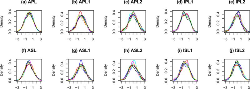
Plots of estimated densities for the transformed residuals from randomly selected locations from each fitted model. The title above each plot indicates the model from which the residuals were taken, with the “1” or “2” indicating the data were fitted to mini-experiments 1 or 2, respectively. This figure demonstrates the near Gaussian character of the transformed residuals, implying the estimated regression coefficients are approximately Gaussian, as required by Assumption A2.

We now consider assumption A3, that the transformed residuals from the fitted model appear to be independent across time. Specifically, after estimating the covariance matrix V(s) at each location using the procedure described in Sec. 3.4 and fitting the desired regression model, the residuals at each location were determined then multiplied by ${\widehat{\mathbf{V}}}^{-1/2}\left(\mathbf{s}\right)$ to obtain the transformed residuals. We applied Ljung-Box tests to the set of transformed residuals from each fitted model at each location for every GCM-RCM combination. We then estimated the empirical CDF of the p-values for each set of transformed residuals. Fig. 4 shows the results for each combination of GCM and RCM, with different colors indicating the different model fits. The black line in each plot indicates the CDF of a standard uniform distribution. An empirical CDF rising above the black line is evidence of a possible problem with the independence assumption for that particular GCM-RCM combination. Nearly all of the empirical CDFs fall below the black line, with the only clear exception being the empirical CDFs of of the CGCM3 GCM. To further assess the potential for problems with the independence assumption, we estimated the proportion of null hypotheses (i.e., the proportion of tests where the transformed residuals were compatible with a sample of independent observations) using the p-values from the Ljeung-Box text using the approach suggested by Storey and Tibshirani (2003). Table 4 provides the estimated proportion of null hypotheses for the GCM-RCM combinations of each regression model. The estimated proportion falls below 1.00 for only three estimates, and these estimates are 0.93, 0.95, and 0.95. This provides additional support that there is little concern that substantive serial dependence remains in the transformed residuals.

Figure 4.

Empirical CDFs of the p-values from the Ljung-Box test of independence of the transformed residuals (across all locations) for each GCM-RCM combination, separated by the model fit. The black line is the CDF of a standard uniform distribution. This figure demonstrates the temporal independence of transformed errors required by Assumption A3.

Table 4.

The proportion of estimated null hypotheses in the Ljeung-Box test of independence for the transformed residuals.

	APL	APL1	APL2	IPL1	IPL2	ASL	ASL1	ASL2	ISL1	ISL2
CCSM-CRCM	1.00	1.00		1.00		1.00	1.00		0.93
CCSM-MM5I	1.00					1.00
CCSM-WRFG	1.00	1.00		1.00		1.00	1.00		1.00
CGCM3-CRCM	1.00	1.00		1.00		1.00	1.00		1.00
CGCM3-RCM3	1.00					1.00
CGCM3-WRFG	1.00	1.00		1.00		1.00	1.00		1.00
GFDL-ECP2	1.00		1.00		1.00	1.00		1.00		1.00
GFDL-HRM3	1.00		1.00		1.00	1.00		1.00		1.00
GFDL-RCM3	1.00					1.00
HadCM3-ECP2	1.00		1.00		1.00	1.00		0.98		0.95
HadCM3-HRM3	1.00		1.00		1.00	1.00		1.00		1.00
HadCM3-MM5I	1.00					1.00

If the transformed residuals violate the independence assumption for a specific GCM-RCM combination, spatial confidence regions for no effect (κ = 0) involving that combination may suffer from undercoverage, meaning the confidence regions are smaller than they should be. Consequently, rejection regions indicating an effect or difference in effect will include more area than they should. Heat maps of significant differences involving GCM-RCM combinations that violate assumption A3 may indicate areas of significant difference when no difference is present.

Lastly, we compare the fitted models using the AIC statistics calculated at each location. Fig. 5 displays the preferred regression model across the spatial domain based on each model’s AIC statistic. Fig. 5 (a) indicates that the APL model is preferred in much of the central and eastern United States as well as the Pacific coastline, while the ASL is preferred near the Sierra and Rocky Mountains and along some of the Atlantic coastline. Fig. 5 (b) indicates that for the mini-experiment 1 data, the simple APL model is generally preferred over other models across most of the United States, with preference for the IPL model in the eastern United States. Lastly, Fig. 5 (c) indicates that for the mini-experiment 2 data, the IPL and ISL models are preferred over most of the United States, with the APL and ASL models being preferred in the southwestern United States. In summary, no clear preference can be given to either the APL or ASL models fitted to the complete data. For the data from mini-experiment 1, the APL model generally seems preferable to either the IPL or ISL models, and for mini-experiment 2, the IPL and ISL models are generally preferred over the APL or ASL models.

Figure 5.

Model preference at each location based on AIC statistics. The coloring indicates which model is preferred for (a) all data, (b) mini-experiment 1 data, and (c) mini-experiment 2 data.

We cannot specifically state why certain models are preferred in some regions over others. However, the temperature behavior varies regionally, so a more complex model may be beneficial in certain regions for modeling the behavior of the data. For the purpose of making simultaneous inference about the effects, we must consider only one class of regression model at a time. Consequently, we will make inference and look at the resulting interpretation for each individual class of regression model.

4.2 Comparison of Effects

We now provide the results from inference related to the effects of the various models. We provide results for pointwise inference at each location (no multiple comparison correction) and from applying the CoPE method. All inference is made at a 0.10 significance level since we had no grounds for a stronger level of Type I error control. The units of all estimated effects is in degrees Celsius.

We begin with inference related to the APL model. First, we determine the locations where the RCM effects significantly differ from each other. More specifically, we are estimating κ(s) = γ_k(s) − γ_l (s) for all possible values of k and l (with k and l denoting the differing RCMs) for the APL model specified in Eq. 1 and determining where this parameter differs from zero. The plots in Figs. 6 and 7 show the results using pointwise inference and the CoPE method, respectively. Only locations where this parameter is significantly different from zero are shown (this is true of subsequent heat maps also). The title above each plot indicates the pairwise difference being estimated.

Figure 6.

A heat map of the estimated average pairwise differences in RCM effect for the APL model. Only significant locations at the 0.10 level using pointwise inference are shown.

Figure 7.

A heat map of the estimated average pairwise differences in RCM effect for the APL model. Only significant locations at the 0.10 level using the CoPE method are shown.

The significant regions are noticeably smaller for the CoPE method, with the interpretation that the region where the effect is non-zero is bounded between the red and blue regions with probability 0.9. The HRM3 and CRCM RCMs are associated with higher warming across the spatial domain in comparison with the other RCMs. In contrast, the ECP2 and MM5I RCMs are associated with a significantly lower warming effect over much of the United States in comparison with the other RCMs. We can formalize this ordering of the models in terms of their overall contribution to the warming signal by integrating the estimated parameter value over the confidence regions and using it as a metric for ranking. (Equivalently, sum over the spatial domain and the columns in each figure to calculate the ranking metric.) These rankings are summarized in Table 5.

Table 5.

Relative overall ordering of model contribution to different components of the warming signal, ordered from highest (top of table) to lowest (bottom of table). The metric used for ordering the models is the integrated estimated parameter value of the pointwise confidence regions. The units for the total warming metric is °C × km² × 10⁶ and the units for the warming rate metric is °C × km² × 10⁶/year.

	Total Warming				Warming Rate
RCM		GCM		RCM		GCM
Model	Metric	Model	Metric	Model	Metric	Model	Metric
HRM3	8.91	GFDL	1.95	MM5I	0.168	GFDL	0.0613
CRCM	6.14	CCSM	1.35	CRCM	0.0595	HadCM3	0.0365
RCM3	1.96	HadCM3	−0.791	HRM3	0.0284	CCSM	−0.0297
WRFG	−3.82	CGCM3	−2.51	RCM3	0.00606	CGCM3	−0.0681
MM5I	−6.47			WRFG	−0.0347
ECP2	−6.73			ECP2	−0.227

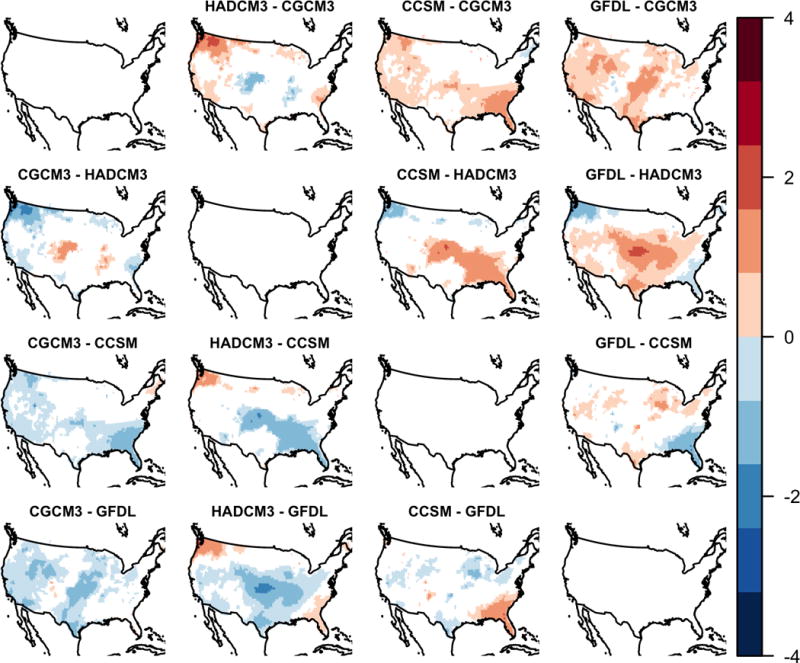
We next determine the locations where the GCM effects significantly differ from each other. Formally, we are estimating κ(s) = β_k(s) − β_l(s) for all possible values of k and l (corresponding to the GCMs) for the APL model specified in Eq. 1. The estimated pairwise differences in GCM effects for the APL models are shown for pointwise inference in Fig. 8 and for the CoPE method in Fig. 9. Using the rank-ordering described above, we can see that CCSM and GFDL GCMs contribute the most to the warming signal, while CGCM3 has the smallest relative contribution.

Figure 8.

A heat map of the estimated average pairwise difference in GCM effect for the APL model. Only significant locations at the 0.10 level using pointwise inference are shown.

Figure 9.

A heat map of the estimated average pairwise difference in GCM effect for the APL model. Only significant locations at the 0.10 level using the CoPE method are shown.

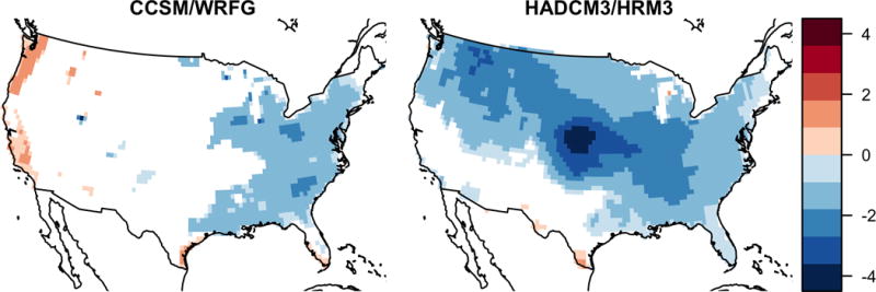
We next assess whether there is a significant interaction effect between the RCMs and the GCMs for the IPL model. More specifically, we are assessing whether δ_ij (s) for the IPL in Eq. 2 is significantly different from zero for the CCSM-WRFG GCM-RCM combination for mini-experiment 1 and the HadCM3-HRM3 combination for mini-experiment 2. A plot of the interaction effect is shown in Fig. 10 for pointwise inference and in Fig. 11 for the CoPE method. There is some evidence of interaction between RCM and GCM using the data available in mini-experiments 1 and 2. Specifically, the CCSM-WRFG model combination shows an additional reduction in warming effect in some regions, and an enhanced warming effect in others, when compared to the main effects of the WRFG and CCSM climate models, respectively. Conversely, the HadCM3-HRM3 model combination tends to estimate overall reduced warming than what is suggested by considering the main effects of HRM3 and HadCM3 models alone.

Figure 10.

A heat map of the estimated average interaction effect for the IPL model. Only significant locations at the 0.10 level using pointwise inference are shown.

Figure 11.

A heat map of the estimated average interaction effect for the IPL model. Only significant locations at the 0.10 level using the CoPE method are shown.

We next proceed to the analysis of the ASL models. For this class of models, we focus on whether there are differences in the rate of temperature change simulated by the climate models. We consider the pairwise differences in the effect on the rate of temperature change for the RCMs and then the GCMs. Specifically, we assess whether η_k (s) − η_l(s) differs from zero for the RCM effects and ζ_k(s) − ζ_l(s) differs from zero for the GCM effects, where k and l vary over all possible combinations of the RCMs and GCMs, respectively. The results for the RCMs are shown in Figs. 12 and 13, and the results for the GCMs are shown in Figs. 14 and 15. Most notably, the regions of significance from the pointwise inference are dramatically larger than those found using the CoPE method. Considering the results for the CoPE analysis, most RCMs do not show significantly different rates of warming. The ECP2 model has a slower rate of warming than the other RCMs in several areas near the mountainous parts of the western U.S., while the MM5I RCM shows evidence of faster warming compared to the other RCMs in various patches of the U.S. However, most of these regions are fairly small, which the expectation that the ECP2 and MM5I models differ significantly in much of the Midwestern states. There is little significant difference in rates of warming between the GCMs except in some coastal areas, particularly along the Gulf of Mexico, where CGCM3 warms more slowly than the other GCMs. Once again, the significant regions from pointwise inference are dramatically larger than those from the CoPE method.

Figure 12.

A heat map of the estimated average pairwise difference in rate of temperature change for RCM effects for the ASL model. Only significant locations at the 0.10 level using pointwise inference are shown.

Figure 13.

A heat map of the estimated average pairwise difference in rate of temperature change for RCM effects for the ASL model. Only significant locations at the 0.10 level using the CoPE method are shown.

Figure 14.

A heat map of the estimated average pairwise difference in rate of temperature change for GCM effects for the ASL model. Only significant locations at the 0.10 level using pointwise inference are shown.

Figure 15.

A heat map of the estimated average pairwise difference in rate of temperature change for GCM effects for the ASL model. Only significant locations at the 0.10 level using the CoPE method are shown.

Lastly, we consider whether there is an interaction effect in the rate of temperature change for the ISL models. In particular, we are assessing whether θ_ij (s) significantly differs from zero for the ISL model in Eq. 4 for the CCSM-WRFG GCM-RCM combination for mini-experiment 1 and the HadCM3-HRM3 combination for mini-experiment 2. There is no evidence of an interaction effect in the rate of temperature change for mini-experiment 1 using either pointwise inference or the CoPE method. For mini-experiment 2, performing pointwise inference suggests a small interaction effect in the rate of temperature change in a few small regions for the HadCM3-HRM3 combination, primarily in Florida and Georgia (not shown). Similarly, for the CoPE method there is only a single location (out of 3,336 locations) that is significant. These results are surprising in light of the AIC statistics shown in Fig. 5. Specifically, for the mini-experiment 1 AIC results shown in Fig. 5 (b), the APL and IPL models (which do not have an interaction effect in the rate of temperature change) were almost universally preferred over the ISL model (which allowed for an interaction effect in the rate of temperature change). On the other hand, for the mini-experiment 2 AIC results shown in Fig. 5 (c), the ISL model was preferred over the IPL model in the locations where the significant interaction effect in rate of temperature change was detected.

5 Discussion

We have utilized four classes of ANOVA-related regression models to compare the effects of the RCMs and GCMs used by the NARCCAP on average summer temperature. The APL model assumes an additive effect for the RCMs and GCMs, but assumes the rate of temperature change is constant for all combinations of models. The IPL model assumes that the average temperature at a location can depend on an interaction between RCMs and GCMs, but the rate of temperature change is constant. The ASL model assumes that the effects of the RCMs and GCMs on the average temperature and on the rate of temperature change are additive. Lastly, the ISL model assumes that the effects of the RCMs and GCMs on the average temperature and on the rate of temperature change can interact.

No one model was preferred over the others, though the APL model tended to be preferred for the data from mini-experiment 1, while the IPL and ISL models tended to be preferred for the data from mini-experiment 2. Figs. 6–15 show the locations where effects differ significantly from zero. This analysis also allows us to rank the RCMs and GCMs in terms of their relative contribution to the warming signal. These rankings are summarized in Table 5. There is convincing evidence that the interaction between the HadCM3 GCM and the HRM3 RCM produces a lower temperature increase than would be suggested by the GCM and RCM individually over a significant portion of the simulation domain. In general, there was little evidence that the RCMs or GCMs differed in their effect on the rate of temperature change. The main exception appears in limited regions when comparing ECP2, which has the lowest contribution to warming, with HRM3 and MM5I, which have the highest contributions to overall warming and to rate of warming, respectively. There was almost no evidence of an interaction effect between the RCMs and GCMs on rate of temperature change.

Due to budgetary constraints, NARCCAP used a fractional factorial experimental design that exercised only half of its 24 possible RCM-GCM combinations. The evidence of a significant interaction effect in certain RCM-GCM combinations highlights the value of carefully constructed experimental designs that explore complete factorial combinations whenever feasible, the substantial limitations of cost inherent to climate model experiments of this magnitude notwithstanding.

We performed inference on the significance of the model effects using both pointwise inference and the CoPE method (Sommerfeld et al., 2015). Pointwise inference does not make any adjustments for multiple comparisons and is designed to control the per-comparison error rate, while the CoPE method is designed to control the familywise error rate. As expected, pointwise inference resulted in significant effects being detected at more locations than the CoPE method: at level α = 0.10, pointwise inference produces an expected false positive area equal to 10% of the area of study with no effect, which is quite large; on the other hand, the CoPE method produces regions that are significantly different from zero with overall probability of 1 − α = 0.9. Sometimes, the difference in the number of significant locations was dramatic, as is evidenced in Figs. 6–15. Additional figures illustrating the size difference of the regions produced by the pointwise and CoPE methods are provided in Figures A1–A5 of the appendix. The CoPE method is a useful method for analyzing climate model effects while ensuring the familywise error rate is appropriately controlled.

6 Code availability

The CoPE method utilized in this manuscript is implemented in the cope R package (Sommerfeld and French, 2016). Computer code for all analysis and plots for this research have been provided as Supplementary Material.

7 Data availability

The bias-corrected NARCCAP data analyzed in this manuscript has been provided as Supplementary Material.

Appendix A

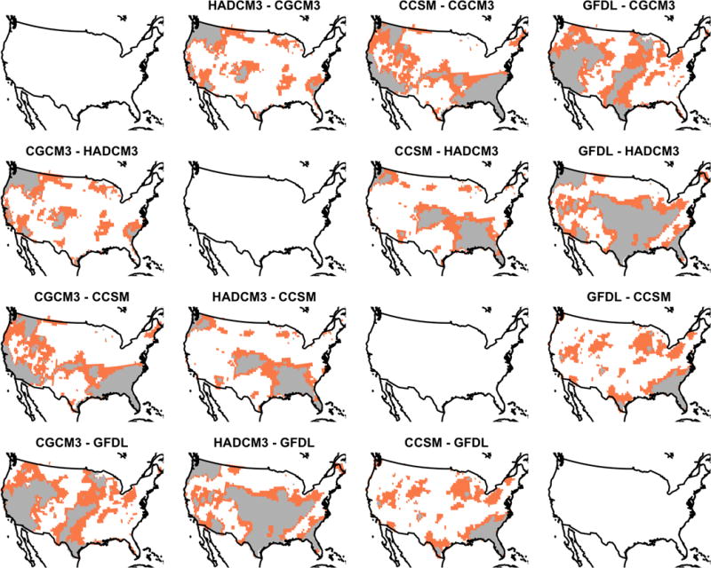
Figure A1.

A comparison of the non-zero effect regions of the average pairwise difference for RCM effects of the APL model using both pointwise and CoPE methods. The grey coloring indicates significant locations at the 0.10 level for both methods, while the orange coloring indicates that the effect is significant for pointwise inference alone.

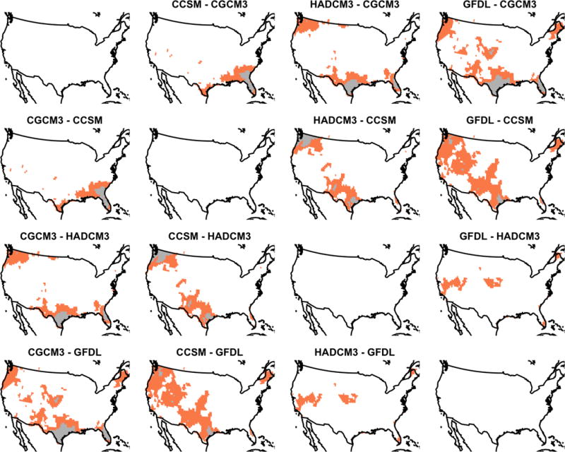
Figure A2.

A comparison of the non-zero effect regions of the average pairwise difference for GCM effects of the APL model using both pointwise and CoPE methods. The grey coloring indicates significant locations at the 0.10 level for both methods, while the orange coloring indicates that the effect is significant for pointwise inference alone.

Figure A3.

A comparison of the non-zero effect regions of the average pairwise difference in rate of temperature change for RCM effects of the ASL model using both pointwise and CoPE methods. The grey coloring indicates significant locations at the 0.10 level for both methods, while the orange coloring indicates that the effect is significant for pointwise inference alone.

Figure A4.

A comparison of the non-zero effect regions of the average pairwise difference in rate of temperature change for GCM effects of the ASL model using both pointwise and CoPE methods. The grey coloring indicates significant locations at the 0.10 level for both methods, while the orange coloring indicates that the effect is significant for pointwise inference alone.

Figure A5.

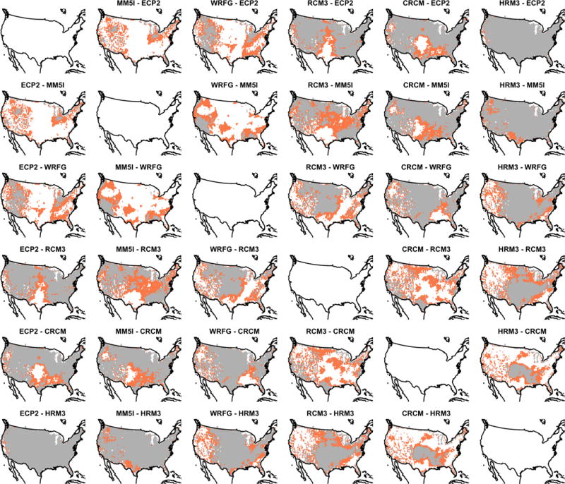
A comparison of the non-zero effect regions of the average interaction effect of the IPL model using both pointwise and CoPE methods. The grey coloring indicates significant locations at the 0.10 level for both methods, while the orange coloring indicates that the effect is significant for pointwise inference alone.

Appendix B: Detailed discussion of covariance estimation

We now describe the estimation process for V(s) in more detail. Exploratory data analysis showed evidence that serial autocorrelation was present for the time series of at least some of the GCM-RCM combinations. Additionally, data exploration suggested that the scale of the errors may change slightly depending on the GCM-RCM combination, though the scale of the errors did not appear to change as a function of time. The size of the data set (up to 358 observations at over 3,000 locations) precluded us from estimating the covariance structure for all locations simultaneously, especially since the dependence structure was not necessarily the same for all GCM-RCM combinations, so the estimation of V(s) was done independently for each location s.

The errors from each GCM-RCM combination were modeled as being independent of errors from a different GCM-RCM combination, with each set of errors modeled using a distinct AR(p_ij) process, where p_ij is the order of the autoregressive process for GCM i and RCM j. Let $ℐ=\left\{\left(i,j\right)\right\}$ be the set of GCM-RCM combinations available in the data for a specific regression model. Then

$$\mathbf{V}\left(\mathbf{s}\right)=\text{diag}\left\{V_{ij}\left(\mathbf{s}\right);\left(i,j\right)\in ℐ\right\},$$ (B1)

i.e., V(s) is the block diagonal of smaller covariance matrices V_ij (s), where V_ij (s) denotes the covariance matrix of the errors for GCM-RCM combination (i,j) at location s. The V_ij(s) are constructed as

$$V_{ij}\left(\mathbf{s}\right):=\mathrm{cov}{\left(Y_{ij{t}_1}\left(\mathbf{s}\right),Y_{ij{t}_2}\left(\mathbf{s}\right)\right)}_{t_1,t_2\in \left\{1,2,\dots ,30\right\}}={\sigma }_{ij}^2{\varphi }_{ij,\left|t_1-t_2\right|,}$$

where |t₁ − t₂| is the time lag between times t₁ and t₂, ${\sigma }_{ij}^2$ is the covariance scaling parameter for GCM-RCM combination (i,j), and ϕ_ij,t. is the correlation between responses having the same GCM-RCM level and separated in time by a lag of t. Note that because the covariance scaling parameter, ${\sigma }_{ij}^2$, was estimated separately for each GCM-RCM combination, this allowed us to account for possible differences in the scale of the errors for each GCM-RCM combination. The parameters of each AR(p_ij) error process were estimated using restricted maximum likelihood estimation under the assumption of Gaussian errors. The autoregressive order for GCM-RCM combination (i,j), p_ij, was chosen independently for each regression model and GCM-RCM combination after considering the correlation structure of the residuals. Table 6 summarizes the order of the autoregressive model fit to the residuals of each regression model for each GCM-RCM combination.

Table 6.

The order of the autoregressive model fit to the residuals of each regression model for each GCM-RCM combination.

	APL	APL1	APL2	IPL1	IPL2	ASL	ASL1	ASL2	ISL1	ISL2
CCSM-CRCM	2	2		2		2	2		2
CCSM-MM5I	0					0
CCSM-WRFG	1	1		1		1	1		1
CGCM3-CRCM	0	0		0		0	0		0
CGCM3-RCM3	1					1
CGCM3-WRFG	0	0		0		0	0		0
GFDL-ECP2	2		2		2	4		4		2
GFDL-HRM3	0		0		0	1		1		1
GFDL-RCM3	0					0
HadCM3-ECP2	0		0		0	1		1		1
HadCM3-HRM3	1		1		1	1		1		1
HadCM3-MM5I	1					1

After the set of estimated covariances matrices $\left\{{\widehat{V}}_{ij}\left(\mathbf{s}\right);\left(i,j\right)\in ℐ\right\}$ were obtained, they were concatenated after the pattern of Eq. (B1) to obtain the complete estimated covariance matrix, $\widehat{\mathbf{V}}\left(\mathbf{s}\right)$. Note that because the mean structure changes for each regression model, V(s) had to be estimated separately in the context of each regression model. Specifically, the $\widehat{\mathbf{V}}\left(\mathbf{s}\right)$ used in analyzing data for the APL regression model was estimated specifically for that model, while separate estimates were obtained for the IPL, ASL, and ISL models, respectively.

We now summarize the covariance estimation process described above in a more algorithmic way. The steps listed below are performed separately for the APL, IPL, ASL, and ISL models. For each location s:

1. Fit the specified regression model (APL, IPL, ASL, or ISL) to the responses at the location using ordinary least squares estimation.

2. Compute the residuals using the fitted model.

3. Separate the residuals into twelve groups based on their associated GCM-RCM combination.

4. Fit an AR(p) model to the residuals from each group using the order p specified in Table 6.

5. Construct the estimated covariance matrix for the residuals of each group using the fitted AR(p) model.

6. Construct the estimated covariance matrix for the complete set of residuals by stacking the estimated covariance matrices for each group into a single block-diagonal matrix.

References

- Akaike H. A new look at the statistical model identification. IEEE Transactions on Automatic Control. 1974;19:716–723. doi: 10.1109/TAC.1974.1100705. [DOI] [Google Scholar]
- Arnold JB. ggthemes: Extra Themes, Scales and Geoms for ’ggplot2’. 2016 https://CRAN.R-project.org/package=ggthemes, r package version 3.0.3.
- Benjamini Y, Heller R. False Discovery Rates for Spatial Signals. Journal of the American Statistical Association. 2007;102:1272–1281. doi: 10.1198/016214507000000941. http://dx.doi.org/10.1198/016214507000000941. [DOI] [Google Scholar]
- Benjamini Y, Hochberg Y. Controlling the False Discovery Rate: A Practical and Powerful Approach to Multiple Testing. Journal of the Royal Statistical Society. Series B (Methodological) 1995;57:289–300. http://www.jstor.org/stable/2346101. [Google Scholar]
- Bolin D, Lindgren F. Excursion and contour uncertainty regions for latent Gaussian models. Journal of the Royal Statistical Society: Series B (Statistical Methodology) 2015;77:85–106. doi: 10.1111/rssb.12055. http://dx.doi.org/10.1111/rssb.12055. [DOI] [Google Scholar]
- Brownrigg R, Minka TP, Deckmyn A. maps: Draw Geographical Maps. 2016 https://CRAN.R-project.org/package=maps, r package version 3.1.0.
- Caya D, Laprise R. A semi-implicit semi-Lagrangian regional climate model: The Canadian RCM. Monthly Weather Review. 1999;127:341–362. [Google Scholar]
- Collins M, Booth BB, Harris GR, Murphy JM, Sexton DM, Webb MJ. Towards quantifying uncertainty in transient climate change. Climate Dynamics. 2006;27:127–147. doi: 10.1007/s00382-006-0121-0. [DOI] [Google Scholar]
- Dahl DB. xtable: Export Tables to LaTeX or HTML. 2016 https://CRAN.R-project.org/package=xtable, r package version 1.8.2.
- Deser C, Phillips A, Bourdette V, Teng H. Uncertainty in climate change projections: the role of internal variability. Climate Dynamics. 2012;38:527–546. doi: 10.1007/s00382-010-0977-x. http://dx.doi.org/10.1007/s00382-010-0977-x. [DOI] [Google Scholar]
- Dowle M, Srinivasan A, Short T, Lianoglou S. data.table: Extension of Data.frame. 2015 https://CRAN.R-project.org/package=data.table, r package version 1.9.6.
- Flato G, et al. The Canadian centre for climate modeling and analysis global coupled model and its climate. Climate Dynamics. 2000;16:451–467. doi: 10.1007/s003820050339. [DOI] [Google Scholar]
- French J. SpatialTools: Tools for Spatial Data Analysis. 2015 http://CRAN.R-project.org/package=spatialtools, r package version 1.0.2.
- French J. autoimage: Display Multiple Images with Scaled Colors. 2016 r package version 0.2.1. [Google Scholar]
- French JP. Confidence regions for the level curves of spatial data. Environmetrics. 2014;25:498–512. doi: 10.1002/env.2295. http://dx.doi.org/10.1002/env.2295. [DOI] [Google Scholar]
- French JP, Hoeting JA. Credible regions for exceedance sets of geostatistical data. Environmetrics. 2016;27:4–14. doi: 10.1002/env.2371. http://dx.doi.org/10.1002/env.2371. [DOI] [Google Scholar]
- French JP, Sain SR. Spatio-temporal exceedance locations and confidence regions. The Annals of Applied Statistics. 2013;7:1421–1449. [Google Scholar]
- Genz A, Bretz F, Miwa T, Mi X, Leisch F, Scheipl F, Hothorn T. mvtnorm: Multivariate Normal and t Distributions. 2016 http://CRAN.R-project.org/package=mvtnorm, r package version 1.0.5.
- GFDL GAMDT (The GFDL Global Atmospheric Model Development Team) The new GFDL global atmospheric and land model AM2-LM2: Evaluation with prescribed SST simulations. Journal of Climate. 2004;17:4641–4673. [Google Scholar]
- Giorgi F, Marinucci MR, Bates GT. Development of a second-generation regional climate model (RegCM2). Part I: Boundary-layer and radiative transfer processes. Monthly Weather Review. 1993a;121:2794–2813. [Google Scholar]
- Giorgi F, Marinucci MR, Bates GT, De Canio G. Development of a second-generation regional climate model (RegCM2). Part II: Convective processes and assimilation of lateral boundary conditions. Monthly Weather Review. 1993b;121:2814–2832. [Google Scholar]
- Gordon C, et al. The simulation of SST, sea ice extents and ocean heat transports in a version of the Hadley Centre coupled model without flux adjustments. Climate Dynamics. 2000;16:147–168. [Google Scholar]
- Grell G, Dudhia J, Stauffer D. A description of the fifth generation Penn State/NCAR Mesoscale Model (MM5) 1993. p. 107. (Tech. rep., National Center for Atmospheric Research, nCAR Technical Note NCAR/TN-398). [Google Scholar]
- Gu H, Zong Z, Hung K. A modified superconvergent patch recovery method and its application to large deformation problems. Finite Elements in Analysis and Design. 2004;40:665–687. doi: http://dx.doi.org/10.1016/S0168-874X(03)00109-4, http://www.sciencedirect.com/science/article/pii/S0168874X03001094. [Google Scholar]
- Hankin RKS. Recreational mathematics with R: introducing the ’magic’ package. R News. 2005;5 [Google Scholar]
- Hill C, DeLuca C, Balaji, Suarez M, Silva AD. The architecture of the Earth System Modeling Framework. Computing in Science Engineering. 2004;6:18–28. doi: 10.1109/MCISE.2004.1255817. [DOI] [Google Scholar]
- Holm S. A simple sequentially rejective multiple test procedure. Scandinavian journal of statistics. 1979:65–70. [Google Scholar]
- Hyndman RJ, Athanasopoulos G. Forecasting: principles and practice. OTexts: Melbourne, Australia; 2013. https://www.otexts.org/fpp/2/6, accessed on 2016-07-22. [Google Scholar]
- IPCC. Emissions Scenarios. Cambridge University Press; Cambridge: 2000. [Google Scholar]
- Jones R, Noguer M, Hassell D, Hudson D, Wilson S, Jenkins G, Mitchell J. Generating high resolution climate change scenarios using PRECIS. Met Office Hadley Centre; Exeter: 2004. [Google Scholar]
- Juang HMH, Hong SY, Kanamitsu M. The NCEP regional spectral model: an update. Bulletin of the American Meteorological Society. 1997;78:2125–2143. [Google Scholar]
- Kaufman CG, Sain SR. Bayesian functional ANOVA modeling using Gaussian process prior distributions. Bayesian Anal. 2010;5:123–149. doi: 10.1214/10-BA505. http://dx.doi.org/10.1214/10-BA505. [DOI] [Google Scholar]
- Khoei A, Gharehbaghi S. The superconvergence patch recovery technique and data transfer operators in 3D plasticity problems. Finite Elements in Analysis and Design. 2007;43:630–648. doi: http://dx.doi.org/10.1016/j.finel.2007.01.002, http://www.sciencedirect.com/science/article/pii/S0168874X07000029. [Google Scholar]
- Klaus B, Strimmer K. fdrtool: Estimation of (Local) False Discovery Rates and Higher Criticism. 2015 https://CRAN.R-project.org/package=fdrtool, r package version 1.2.15.
- Ljung G, Box G. On a measure of lack of fit in time series models. Biometrika. 1978;65:297–303. doi: 10.1093/biomet/65.2.297. [DOI] [Google Scholar]
- Maurer EP, Brekke L, Pruitt T, Duffy PB. Fine resolution climate projections enhance regional climate change impact studies. EOS, Transactions American Geophysical Union. 2007;88:504–504. [Google Scholar]
- McGinnis S, Nychka D, Mearns LO. Machine Learning and Data Mining Approaches to Climate Science. Springer International Publishing; 2015. A new distribution mapping technique for climate model bias correction; pp. 91–99. [Google Scholar]
- Mearns LO, Gutowski W, Jones R, Leung R, McGinnis S, Nunes A, Qian Y. A regional climate change assessment program for North America. EOS, Transactions American Geophysical Union. 2009;90:311–311. [Google Scholar]
- Mearns LO, Arritt R, Biner S, Bukovsky MS, McGinnis S, Sain S, Caya D, Correia J, Jr, Flory D, Gutowski W, et al. The North American regional climate change assessment program: overview of phase I results. Bulletin of the American Meteorological Society. 2012;93:1337–1362. [Google Scholar]
- Meehl G, et al. Climate Change 2007: The Physical Science Basis—Contribution of Working Group 1 to the Fourth Assessment Report of the Intergovernmental Panel on Climate Change. Cambridge University Press; New York: 2007. Global climate projections; pp. 747–843. chap. 10. [Google Scholar]
- Murdoch DJ, Tsai YL, Adcock J. P-Values are Random Variables. The American Statistician. 2008;62:242–245. http://0-www.jstor.org.skyline.ucdenver.edu/stable/27644033. [Google Scholar]
- National Center for Atmospheric Research. Regridding using NCL with Earth System Modeling Framework (ESMF) software. 2017 http://www.ncl.ucar.edu/Applications/ESMF.shtml, accessed on March 22, 2017.
- Neuwirth E. RColorBrewer: ColorBrewer Palettes. 2014 https://CRAN.R-project.org/package=RColorBrewer, r package version 1.1.2.
- Nychka D, Furrer R, Paige J, Sain S. fields: Tools for Spatial Data. 2016 https://CRAN.R-project.org/package=fields, r package version 8.3.6.
- Pinheiro J, Bates D, DebRoy S, Sarkar D, R Core Team nlme: Linear and Nonlinear Mixed Effects Models. 2016 http://CRAN.R-project.org/package=nlme, r package version 3.1.127.
- Plate T, Heiberger R. abind: Combine Multidimensional Arrays. 2015 https://CRAN.R-project.org/package=abind, r package version 1.4.3.
- Pope V, Gallani M, Rowntree P, Stratton R. The impact of new physical parametrizations in the Hadley Centre climate model: HadAM3. Climate Dynamics. 2000;16:123–146. [Google Scholar]
- R Core Team. R: A Language and Environment for Statistical Computing. R Foundation for Statistical Computing; Vienna, Austria: 2016. https://www.R-project.org/ [Google Scholar]
- Sain SR, Nychka D, Mearns L. Functional ANOVA and regional climate experiments: a statistical analysis of dynamic downscaling. Environmetrics. 2011;22:700–711. doi: 10.1002/env.1068. http://dx.doi.org/10.1002/env.1068. [DOI] [Google Scholar]
- Scinocca J, McFarlane N. The variability of modeled tropical precipitation. Journal of Atmospheric Science. 2004;61:1993–2015. [Google Scholar]
- Shen X, Huang HC, Cressie N. Nonparametric hypothesis testing for a spatial signal. Journal of the American Statistical Association. 2002;97:1122–1140. [Google Scholar]
- Skamarock WC, Klemp JB, Dudhia J, Gill DO, Barker DM, Wang W, Powers JG. A description of the advanced research WRF version 2. 2005. (Tech. rep., National Center for Atmospheric Research, nCAR Technical Note NCAR/TN-468+STR). [Google Scholar]
- Sommerfeld M, French JP. cope: Coverage Probability Excursion (CoPE) Sets. 2016 r package version 0.2. [Google Scholar]
- Sommerfeld M, Sain S, Schwartzman A. Confidence regions for excursion sets in asymptotically Gaussian random fields, with an application to climate. 2015 doi: 10.1080/01621459.2017.1341838. arXiv preprint arXiv 1501.07000. [DOI] [PMC free article] [PubMed] [Google Scholar]
- Storey JD, Tibshirani R. Statistical significance for genome-wide experiments. Proceedings of the National Academy of Sciences. 2003;100:9440–9445. doi: 10.1073/pnas.1530509100. [DOI] [PMC free article] [PubMed] [Google Scholar]
- Sun W, Reich BJ, Tony Cai T, Guindani M, Schwartzman A. False discovery control in large-scale spatial multiple testing. Journal of the Royal Statistical Society: Series B (Statistical Methodology) 2015;77:59–83. doi: 10.1111/rssb.12064. http://dx.doi.org/10.1111/rssb.12064. [DOI] [PMC free article] [PubMed] [Google Scholar]
- Teutschbein C, Seibert J. Bias correction of regional climate model simulations for hydrological climate-change impact studies: Review and evaluation of different methods. Journal of Hydrology. 2012:456–457. 12–29. doi: http://dx.doi.org/10.1016/j.jhydrol.2012.05.052, http://www.sciencedirect.com/science/article/pii/S0022169412004556.
- Venables WN, Ripley BD. fourth. Springer; New York: 2002. Modern Applied Statistics with S. http://www.stats.ox.ac.uk/pub/MASS4. [Google Scholar]
- Weisberg S. Applied Linear Regression. 4th. Wiley; Hoboken: 2014. [Google Scholar]
- Wickham H. ggplot2: Elegant Graphics for Data Analysis. Springer-Verlag; New York: 2009. http://ggplot2.org. [Google Scholar]
- Wilks DS. Statistical Methods in the Atmospheric Sciences. Vol. 100. Academic Press; 2011. [Google Scholar]