Split probabilities and species tree inference under the multispecies coalescent model

Abstract

Using topological summaries of gene trees as a basis for species tree inference is a promising approach to obtain acceptable speed on genomic-scale datasets, and to avoid some undesirable modeling assumptions. Here we study the probabilities of splits on gene trees under the multispecies coalescent model, and how their features might inform species tree inference. After investigating the behavior of split consensus methods, we investigate split invariants — that is, polynomial relationships between split probabilities. These invariants are then used to show that, even though a split is an unrooted notion, split probabilities retain enough information to identify the rooted species tree topology for trees of 5 or more taxa, with one possible 6-taxon exception.

1 Introduction

As advances in technology have allowed for the collection of genomic scale data across a collection of organisms, it has been frequently observed that phylogenetic trees inferred from single genes for a fixed taxon set often differ from one another. Improving inference of species relationships requires addressing such gene tree discordance in a principled way. While there are several biological processes that might cause this discord, including hybridization or other forms of horizontal gene transfer, incomplete lineage sorting is an especially common source of gene tree incongruence when times between speciation events are short and/or population sizes are large. Incomplete lineage sorting is modeled by the the multispecies coalescent model, an extension of the standard coalescent model describing gene tree formation within a single population.

Many methods of species tree inference based on the multspecies coalescent have been proposed. The Baysian approaches of the software *BEAST [HD10] and Mr. Bayes/BEST [LP07,RTvdM⁺12] perform simultaneous gene tree and species tree inference under a combined coalescent and sequence evolution model, from data composed of the site pattern frequencies for individual genes. The SVDquartets method [CK15,LK17] also utilizes a combined model, but bases inference on site pattern frequencies across the full genome, with no assignment of sites to genes. Nonetheless it still gives a statistically consistent estimate of the species tree under the plausible assumption of independence of gene length and gene tree.

Alternatively, gene trees inferred by traditional phylogenetic methods can be used as input for a subsequent inference of a species tree, in methods such as Rooted triple Consensus [EESvH08], STEM [KCK09], STAR [LYPE09], NJ_st/U-STAR/ASTRID [LY11,ADR17,VW15], MP-EST [LYE10], BUCKy [LKDA10] and ASTRAL-II [MW15]. While theoretical justification for these two-stage approaches generally ignores gene tree inference error, they can be applied to much larger data sets (more taxa and more genes) than the computationally intensive Bayesian algorithms, and have exhibited strong performance in simulations. Such scalability makes them highly attractive, and motivates further exploration of their underpinnings.

A fundamental issue for any inference of a species tree is how to relate the time scale used in the multispecies coalescent model on a species tree to those in sequence evolution models used on gene trees. The coalescent time scale can be measured in number of generations divided by population size, while the sequence evolution model is generally in number of substitutions per site. Assumptions such as a constant mutation rate over the gene tree (implying all gene trees are ultrametric) and a constant population size over the species tree are sometimes made, despite their implausibility. While these assumptions can be relaxed somewhat through more elaborate modeling, it is difficult to test the robustness of inference when they are violated.

An alternative way of addressing this difficult time scale issue is to simply discard all metric information inferred about gene trees, and only use their topological features to infer a species tree. Although discarding such information is undesirable if one can validly relate time scales, one can view it as a conservative approach to avoid reliance on unjustified assumptions.

Some methods go further, and only consider summaries of the inferred topological gene trees, such as displayed quartets (unrooted 4-taxon trees), rooted triples (rooted 3-taxon trees), clades (all taxa descended from an internal node of the rooted tree) or splits (bipartitions of taxa induced by an edge in the tree). Among current methods, Rooted triple consensus, MP-EST, BUCKy, STAR, ASTRAL-II, and NJ_st/U-STAR/ASTRID are all of this type. (While for Rooted triple Consensus, MP-EST, BUCKy and ASTRAL-II this is obvious from their formulations, for STAR and NJ_st the connection to clades and splits was established in [ADR13] and [ADR17].) These methods all use topological summaries of a sample of gene trees, rather than the full trees, in ways allowing for statistically consistent species tree inference when the gene trees are sampled from the multispecies coalescent model without error.

In this work, we undertake a theoretical study of the probabilities of splits on gene trees arising from the multispecies coalescent, with the aim of better understanding how species tree inference may be performed from gene tree split information. This parallels several previous works, in which we have shown that rooted species tree topologies are identifiable from unrooted gene tree topologies or from clades displayed on gene trees, and unrooted species tree topologies are identifiable from gene tree quartets.

A pleasant outcome of our study is that gene tree split probabilities generally retain enough information on the species tree that they determine both its topology and its root, despite the fact that splits themselves are an unrooted notion. Specifically, for all species trees on 5 or more taxa, with one 6-taxon exception, for generic edge lengths, the rooted species tree topology is identifiable. Translating to an empirical setting, this means that one should be able to develop a statistically consistent method of inference of the rooted species tree from the frequencies of splits on a collection of unrooted gene trees. This would be an extension of the NJ_st/U-STAR/ASTRID method, which only infers an unrooted species tree topology from the same information. Such a method would avoid any issues with erroneous rooting of gene trees by inclusion of an outgroup, which has long been known as a source of additional error (see [PBL⁺11] for a recent discussion), and allow rooting even when no appropriate outgroup is available. A recent work [AD17] pursued this through approximate Bayesian computation, with split distributions used as one measure to estimate a posterior distribution of rooted species trees. Since the method by which we show the species tree root is identifiable depends only on linear relationships between split probabilities, other approaches taking advantage of this simple form may also be possible.

After setting notation in Section 2, we begin our study of split probabilities under the multispecies coalescent in Section 3 with some basic observations. These include an analysis of the behavior of greedy split consensus from gene tree splits, concluding that it is not a statistically consistent method of species tree inference even on trees with as few as 5 taxa. Mathematical arguments for this appear in Appendix A.

Since split probabilities are complicated expressions that are difficult to compute for trees with more than 6 taxa, in Section 4 we turn our attention to relationships between such split probabilities — that is, rather than focus on explicit formulas for them, we look for implicit formulas they must satisfy. Our methods thus are mathematically the same as those used for studying pattern probabilities under sequence evolution models through phylogenetic invariants, so we adopt the same terminology of referring to equalities as invariants. Our previous work [ADR17] on relationships between the split probabilities and the NJ_st/U-STAR/ASTRID inference method quickly leads to a number of linear invariants and inequalities the split probabilities must satisfy, tied to the quartets displayed on the species tree. These depend only on the unrooted species tree, and thus give no information on its root. However, building on results in [ADR11a], we then find additional split invariants that depend on the clades displayed on the species tree, which thus give some information about the root location. While our theoretical work gives only linear invariants, independent invariants of higher degree also exist. Unfortunately a computational determination of them was successful only for 5-taxon trees, and their structure remains unclear.

In Section 5 we build on the results on linear invariants from Section 4, to prove a main result: the collection of split probabilities under the multispecies coalescent model determines the species tree topology, including the root location (with one exception). This identifiability result, Theorem 3, holds generically, i.e., for all edge lengths on the species tree not in a set of measure zero. For most trees testing whether the invariants found in the previous section vanish is sufficient for locating the root; however, for certain trees these tests leave several possibilities for the branching pattern near the root of the tree. Motivated by known invariants, we formulate some linear inequalities that resolve these ambiguities in all cases, except for a particular unrooted 6-taxon tree shape. Establishing that these inequalities hold is accomplished by a laborious technical argument, which is relegated to Appendix B.

2 Notation

Let 𝒳 be a finite set of taxa, whose elements are denoted by lower case letters a, b, c, … etc. For any specific gene, we denote a single sample from each taxon by the corresponding upper case letter A, B, C, … etc. If 𝒜 ⊆ 𝒳 is a subset of taxa, the corresponding subset of genes is 𝒜_g ⊆ 𝒳_g.

By a species tree σ = (ψ, λ) on 𝒳 we mean a rooted topological phylogenetic tree ψ, with leaves bijectively labelled by 𝒳, together with an assignment of edge weights λ to its internal edges. These edge weights are specified in coalescent units, so that the multispecies coalescent model on σ leads to a probability distribution on rooted gene trees with leaves labelled by 𝒳_g. (For more on the multispecies coalescent model as we use it, see [ADR11b].) Since we limit ourselves to the situation where one individual is sampled per taxon, no coalescent events can occur in pendant edges of a species tree, so the lengths of those edges are inconsequential and omitted from our notation. (If more than one individual is sampled per taxon, one can create an “extended species tree” as in [ADR11a] by grafting several pendant edges of unspecified length to the leaf labeled by that taxon, and assigning a length to the formerly pendant edge, to again be in the framework set here.)

The gene trees sampled from the coalescent are rooted metric binary phylogenetic trees on 𝒳_g, though marginalization over edge lengths and root locations induces a distribution on unrooted topological binary gene trees. Unrooted topological gene trees will be denoted by T, and the probability of an unrooted topological gene tree under the multispecies coalescent on σ is denoted by ℙ_σ(T), or simply ℙ(T) when σ is clear from context.

A split of a set of taxa 𝒳 is a bipartition 𝒜 ⊔ ℬ into nonempty subsets, denoted 𝒜|ℬ = ℬ|𝒜 = Sp(𝒜) = Sp(ℬ). If σ is a species tree on 𝒳 then by a split on σ we mean a split of 𝒳 formed by deleting a single edge of ψ and grouping taxa according to the connected components of the resulting graph. We similarly refer to splits of 𝒳_g, and splits of 𝒳_g on specific gene trees T. For small sets of taxa, it will often be convenient to use juxtaposition of elements to represent sets, rather than standard set notation. Thus ac = {a, c} and Sp(ac) = Sp({a, c}).

In a trivial split, one of the partition blocks is a singleton set. Trivial splits for taxa 𝒳 appear on every phylogenetic tree on 𝒳. For 𝒜 ⊂ 𝒳 we will denote the complementary set of 𝒜 by 𝒜̄ = 𝒳 \ 𝒜, so that 𝒜|𝒜̄ is a split when ∅ ≠ 𝒜 ⊊ 𝒳.

For a species tree σ on 𝒳, by the probability of a split 𝒜|ℬ of 𝒳 under the multispecies coalescent we mean

$${\mathbb{P}}_{\sigma }(\mathcal{A}\mid \mathcal{B})=\sum _T{\mathbb{P}}_{\sigma }(T){\delta }_{\mathcal{A}\mid \mathcal{B}}(T)$$ (1)

where δ_𝒜|ℬ(T) is 1 if 𝒜_g|ℬ_g is a split on T, and 0 otherwise, and the sum runs over all binary unrooted topological phylogenetic trees on 𝒳_g. Thus the probability of a split is the probability that an observation of a gene tree displays the corresponding split. Note that trivial splits have probability 1 for every species tree, since they are on every binary gene tree.

We will also need to refer to clades and quartets of taxa. A clade is simply a subset 𝒜 ⊆ 𝒳. A clade 𝒜 is on the species tree σ if it equals the set of all leaf-descendants of some node in the tree. A quartet is a 4-element subset of 𝒳 partitioned into 2-element sets, denoted as ab|cd, with a, b, c, d ∈ 𝒳. A quartet ab|cd is on σ if the unrooted tree with leaves labeled a, b, c, d induced from σ has an edge separating a, b from c, d.

Finally, given a rooted topological tree on 𝒳, and a subset 𝒴 ⊆ 𝒳, we use MRCA(𝒴) to denote the most recent common ancestor of 𝒴, i.e., the least ancestral node in the tree which is ancestral to all elements of 𝒴. For a node v in the tree, we use desc_𝒳(v) to denote the set of taxa descended from v. Thus a clade 𝒴 ⊆ 𝒳 is on the tree if and only if 𝒴 = desc_𝒳(MRCA(𝒴)).

3 Basic observations

While in principle it is straightforward to compute the probabilities of gene tree splits for a fixed species tree, in practice the work required can be formidable. For an n-taxon species tree, using the definition in equation (1), one first must compute probabilities of each of the (2n − 3)!! = 1 · 3 ··· (2n − 3) unrooted topological gene trees. This can be accomplished by work of [DS05] or [Wu12] in finding probabilities of all rooted topological gene trees, and then marginalizing over the root locations. For a given split one must still sum over all unrooted gene trees displaying that split. If the split has blocks of size k and n − k, then there are (2k − 3)!! (2n − 2k − 3)!! such unrooted trees.

Using this approach, we computed split probabilities for all species trees on 6 or fewer taxa for use in computations discussed in later sections, but went no further. Indeed, this approach does not seem to be tractable except for small species trees. On the other hand, since the U-STAR inference methods implemented in ASTRID are based on split frequencies [VW15,ADR17] and perform well on large data sets, theoretical study of these probabilities is still strongly warranted.

As a first step, analogous to Proposition 1 of [ADR11a] for clade probabilities, we have the following.

Lemma 1

If |𝒳| = n, then the sum of the non-trivial split probabilities is n − 3.

Proof

First considering all splits of 𝒳, including trivial ones,

$$\begin{gathered} \sum _{\mathcal{A}\mid \mathcal{B}}{\mathbb{P}}_{\sigma }(\mathcal{A}\mid \mathcal{B})=\sum _{\mathcal{A}\mid \mathcal{B}}\sum _T{\mathbb{P}}_{\sigma }(T){\delta }_{\mathcal{A}\mid \mathcal{B}}(T)=\sum _T{\mathbb{P}}_{\sigma }(T)\sum _{\mathcal{A}\mid \mathcal{B}}{\delta }_{\mathcal{A}\mid \mathcal{B}}(T) \\ =\sum _T{\mathbb{P}}_{\sigma }(T)(2n-3)=2n-3. \end{gathered}$$

Since the n trivial splits of 𝒳 all have probability 1, removing them from the sum gives the claim.

Another analog of a result for clade probabilities, Theorem 3 of [ADR11a], is the content of the next Proposition. T. Warnow first asked if this might hold, and C. Ané independently provided a proof [Ané].

Proposition 1

Let ε ≥ 0 be fixed, and let σ be a binary species tree on 𝒳 with internal edge lengths λ_i > ε. Consider any split 𝒜|ℬ of 𝒳.

Then under the multispecies coalescent model if

$${\mathbb{P}}_{\sigma }(\mathcal{A}\mid \mathcal{B})\ge (1/3)exp(-\epsilon )$$

then 𝒜|ℬ is displayed on σ.

Furthermore, if (1/3) exp(−ε) is replaced with any smaller number, this statement is no longer true: For any α < (1/3) exp(−ε), there exists a species tree σ with branch lengths λ_i > ε and a split 𝒜|ℬ of 𝒳 not displayed on σ with ℙ_σ(𝒜|ℬ) > α.

Proof

The first statement holds for trivial splits, since they have probability 1 and are displayed on every binary σ.

Now consider a non-trivial split 𝒜|ℬ not displayed on σ. Then there exist a₁, a₂ ∈ 𝒜, b₁, b₂ ∈ ℬ so the quartet a₁a₂|b₁b₂ is not displayed on σ. Thus, by [ADR11b, Section 4.1] the probability that an unrooted gene tree displays the quartet A₁A₂|B₁B₂ is

$${\mathbb{P}}_{\sigma }({\mathit{\Lambda }}_1{\mathit{\Lambda }}_2\mid B_1{B}_2)=(1/3)exp(-\ell )<(1/3)exp(-\epsilon )$$

where ℓ > ε is the sum of the lengths of all branches in σ that form the central edge in the induced quartet tree on a₁, a₂, b₁, b₂. But since displaying the split 𝒜_g|ℬ_g is a subevent of displaying A₁A₂|B₁B₂, this implies that if 𝒜|ℬ is not displayed on σ then

$${\mathbb{P}}_{\sigma }(\mathcal{A}\mid \mathcal{B})<(1/3)exp(-\epsilon ),$$

establishing the first claim.

For the second claim, we construct an example. For any non-trivial split 𝒜|ℬ, pick a ∈ 𝒜, b ∈ ℬ, and let 𝒜′ = 𝒜 \ {a}, ℬ′ = ℬ \ {b}. Pick any binary rooted tree σ₁ on 𝒜′, and any binary rooted tree σ₂ on ℬ′, with internal branch lengths greater than ε, and consider the tree

$$\sigma =(((a,b):{\lambda }_1,{\sigma }_1:{\lambda }_2):{\lambda }_3,{\sigma }_2:{\lambda }_4).$$

Note 𝒜|ℬ is not a split on this tree. However, if λ₂, λ₄ are sufficiently large, then the lineages for each of the groups ${\mathcal{A}}_g^{\prime }$ and ${\mathcal{B}}_g^{\prime }$ are almost certain to have coalesced within the branches of those lengths. But then using results on the probabilities of unrooted topological gene trees for 4-taxon species trees from [ADR11b], we deduce that the probability of a gene tree displaying the split 𝒜_g|ℬ_g can be made arbitrarily close to (1/3) exp(−λ₁). If α < (1/3) exp(−ε), there is a choice of λ₁ > ε so that α < (1/3) exp(−λ₁). Thus we can ensure ℙ_σ(𝒜|ℬ) > α.

Setting ε = 0 in the previous proposition yields the following.

Corollary 1

Suppose σ is a binary species tree on 𝒳, with positive edge lengths, and 𝒜|ℬ a split of 𝒳. Then under the multispecies coalescent model if

$${\mathbb{P}}_{\sigma }(\mathcal{A}\mid \mathcal{B})\ge 1/3$$

then 𝒜|ℬ is a split on σ.

This proposition has implications for a greedy split consensus approach to inferring splits in a species tree. Recall that in this method, one first orders splits observed in a gene tree sample by decreasing frequency, arbitrarily (or randomly) breaking ties if necessary. Proceeding in order down the list, splits are accepted if they are compatible with all previously accepted ones. For a large sample of gene trees from the multispecies coalescent, a fully-resolved unrooted tree is likely to be returned, since all splits have positive probability. The above corollary implies that if one only allows the acceptance of splits of frequency greater than 1/3, then this method will not be misleading; as the size of the gene tree sample grows, the probability of accepting only splits on the species tree goes to 1. While a tree displaying the accepted splits may not be fully resolved, one can have confidence in the splits that are displayed.

To show that accepting splits below a frequency 1/3 cutoff in greedy split consensus would not lead to consistent species tree inference, we investigate 5-taxon trees in more detail. Up to permutation of taxon labels, there are three species trees to consider:

$$\begin{array}{ll}\text{balanced}\text{tree}\hfill & {\sigma }_{\mathit{bal}}=(((a,b):x,c):y,(d,e):z)\hfill \\ \text{pseudocaterpillar}\text{tree}\hfill & {\sigma }_{ps}=(((a,b):x,(d,e):y):z,c)\hfill \\ \text{caterpillar}\text{tree}\hfill & {\sigma }_{\mathit{cat}}=((((a,b):x,c):y,d):z,e)\hfill \end{array}$$

Although we use the same variables x, y, z to denote the three internal edge lengths in each tree, note that these have no relationship across the species trees. All split probabilities can be expressed as polynomials in the transformed edge lengths

$$X=exp(-x),Y=exp(-y),Z=exp(-z).$$

Note that with this transformation, values of X close to 1 correspond to small branch lengths x, and values of X close to 0 correspond to large branch lengths x.

The following two propositions are proved in Appendix A.

Proposition 2

For the 5-taxon balanced and pseudocaterpillar species trees, σ = σ_bal, σ_ps, with positive branch lengths,

$${\mathbb{P}}_{\sigma }(Sp(ab)),{\mathbb{P}}_{\sigma }(Sp(de))>{\mathbb{P}}_{\sigma }(\mathcal{S})$$

for each of the eight other non-trivial splits 𝒮, so the splits displayed on the species tree have the highest probability of appearing on gene trees.

When restricted to these species trees, as the sample size goes to infinity greedy split consensus infers the correct unrooted species tree topology with probability approaching 1.

Proposition 3

For the 5-taxon caterpillar species tree σ = σ_cat with positive branch lengths, ℙ_σ(Sp(ab)) > ℙ_σ(𝒮) for all non-trivial splits 𝒮 ≠ Sp(de), and ℙ_σ(Sp(de)) > ℙ_σ(Sp(ce)).

If ℙ_σ(Sp(de)) > ℙ_σ(Sp(cd)) for such a species tree, as the sample size goes to infinity greedy split consensus infers the correct unrooted species tree topology with probability approaching 1.

However, if ℙ_σ(Sp(de)) < ℙ_σ(Sp(cd)), it infers the incorrect unrooted species tree topology ((a, b), e, (c, d)) with probability approaching 1. The parameter region in which this occurs is

$$18+X{Y}^3{Z}^6+2X{Y}^3-3XY-18Y<0.$$ (2)

Figure 1 shows the surface dividing the regions of parameter space on which greedy split consensus is misleading from that on which it is not. We refer to the region behind the surface, in which greedy consensus on splits is expected to return the incorrect species tree, as the too-greedy zone.

Fig. 1.

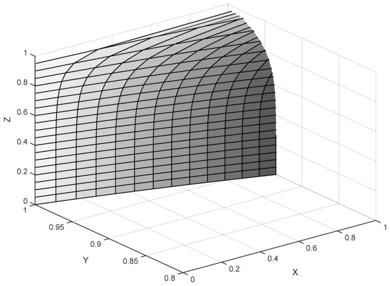
The boundary of the too-greedy zone for the 5-taxon caterpillar tree σ_cat. Greedy consensus for split probabilities is inconsistent for all choices of parameters behind the surface, and consistent in front of the surface. For example, if (X, Y, Z) ≈ (.9, .96, .5), so species tree branch lengths are (x, y, z) ≈ (0.1054, 0.0408, 0.6931), then greedy consensus with a large number of gene trees is expected to return the incorrect tree ((a, b), e, (c, d)).

The analogous expression for the boundary of the five-taxon unrooted anomaly zone (the branch lengths for which the most likely unrooted gene tree does not match the unrooted caterpillar species tree) is ([Deg13], equation (4))

$$18+X{Y}^3{Z}^6+2X{Y}^3+9XY-12X-18Y<0.$$ (3)

We note that if inequality (2) holds, then inequality (3) holds as well. This means that for the five-taxon caterpillar, the too-greedy zone is a subset of the unrooted anomaly zone. This relationship is also true for the rooted 4-taxon caterpillar case: the rooted too-greedy zone is a subset of the rooted anomaly zone. In both the rooted and unrooted cases for four and five taxa, respectively, when greedy consensus is misleading, it returns the anomalous gene tree. We leave it as an open question whether the too-greedy zones for larger trees are also subsets of the corresponding anomaly zones.

One can show that the minimum value of Y on the boundary surface in Figure 1 occurs when X = 1, Y ≈ 0.93498735, and Z = 0, so x = 0, y ≈ 0.06722228, z = ∞. For values of y larger than this, regardless of the values of x and z, branch length parameters are outside the too-greedy zone, and greedy split consensus is expected to return the correct species tree.

Moreover, if Z = 0 so that z is an infinite branch length in σ_cat, the too-greedy zone for splits coincides exactly with the too-greedy zone for clade consensus on the 4-taxon tree (((a, b), c), d) [DDBR09]. This is as expected, since placing the root of the 5-taxon caterpillar species tree “at infinity” makes non-trivial splits for it correspond exactly to clades in the 4-taxon caterpillar, by viewing e as an outgroup and noting that the lineage from e must coalesce last.

As was pointed out to us [Ané], the shape of the surface in Figure 1 has an interesting consequence. As Z increases from 0 to 1, the too-greedy zone in the XY -plane becomes smaller. Equivalently, in terms of branch lengths, as z increases from 0 to ∞, the too-greedy zone in the xy plane becomes larger, as shown in Figure 2. Thus smaller values of z result in greedy split consensus performing well for more choices of branch lengths x and y.

Fig. 2.

For z = 0.01, .05, .1, .5, 1, curves giving, from bottom to top, the boundary of the too-greedy zone in the xy-plane for the 5-taxon caterpillar tree. Note x, y, z are edge lengths in coalescent units. The too-greedy zone for a value of z is the region below the curve, illustrating that the region grows with z. For z > 1 the curve is visually indistinguishable from that for z = 1.

If one views the taxon e as an outgroup on σ_cat, this means that an outgroup that is closely related to all other taxa results in better performance of greedy split consensus than one that is more distantly related. While an extremely distantly related outgroup (z = ∞) enables determination of the root of each gene tree, so that knowing the splits on 5-taxon gene trees is equivalent to knowing the clades on 4-taxon trees omitting the outgroup, this actually reduces the ability of greedy split consensus to determine the correct unrooted topology of the species tree. Indeed, the too-greedy zone for clade consensus on a 4-taxon caterpillar as shown in Figure 3 of [DDBR09] matches precisely that for z = ∞ in Figure 2.

These comments have analogs for the unrooted anomaly zones for five taxa. In particular, the left side of inequality (3) is decreasing in z, so that increasing that branch length results in more values of x and y with (x, y, z) in the anomaly zone.

4 Linear invariants and inequalities for split probabilities

A useful concept for understanding probabilistic models in phylogenetics has been that of a phylogenetic invariant. An invariant of this sort is a multivariate polynomial that when evaluated at probabilities arising from the model gives 0, regardless of the particular parameter values associated to the model instance. Equivalently, it is a polynomial relationship between the probabilities that holds for all parameter values, and thus gives information about the probabilities implicitly.

A split invariant for a species tree topology is a polynomial in the probabilities of splits under the multispecies coalescent model that vanishes for all edge length assignments to the species tree. More completely, a split invariant associated to an n-taxon species tree topology ψ is a multivariate polynomial in 2ⁿ⁻¹ − 1 indeterminates (one for every split) which evaluates to zero at any vector of split probabilities ℙ_σ(𝒜|ℬ) arising from σ = (ψ, λ), regardless of the values of λ. Since probabilities of trivial splits are always 1 under the coalescent, we can and will consider only invariants in variables for the 2ⁿ⁻¹ − n − 1 non-trivial splits.

The trivial split invariant, which is valid for all ψ, is

$$n-3-\sum _{\begin{array}{c}\text{non-trival}\\ \text{splits}\mathcal{A}\mid \mathcal{B}\end{array}}{\mathbb{P}}_{\sigma }(\mathcal{A}\mid \mathcal{B}).$$ (4)

That this evaluates to 0 when the split probabilities arise from the multispecies coalescent on some species tree is established by Lemma 1.

4.1 Linear invariants and inequalities for unrooted species trees

In this section we explore linear relationships, both invariants and inequalities, between split probabilities that are tied to the U-STAR algorithm [ADR17]. Since U-STAR allows a distance method to be used to infer a species tree, these have a rather direct correspondence to equalities and inequalities defining tree metrics.

From equation (7) of [ADR17], we know the expected U-STAR distance on a species tree σ under the multispecies coalescent can be expressed as

$$D(a,b)=\sum _{\begin{array}{c}\text{splits}\mathcal{A}\mid \mathcal{B}\\ \text{separating}a,b\end{array}}{\mathbb{P}}_{\sigma }(\mathcal{A}\mid \mathcal{B}),$$

where a split is said to separate two taxa if they lie in different sets of the bipartition. Moreover, the expected U-STAR distance is a tree metric on σ. Using this in the 4-point condition for tree metrics implies a collection of linear equalities and inequalities in split probabilities that must hold for unrooted species trees. That is, these equalities and inequalities hold regardless of the location of the root on the species tree.

To state the result, we will say that a split 𝒜|ℬ of 𝒳 separates two nonempty disjoint subsets 𝒴₀, 𝒴₁ ⊂ 𝒳 provided 𝒴_i ⊆ 𝒜 and 𝒴_1−i ⊆ ℬ for one of i = 0, 1.

Theorem 1

Suppose σ is an n-taxon species tree on 𝒳, and a, b, c, d ∈ 𝒳 are any four taxa for which σ induces the quartet tree ab|cd. Then

$$\sum _{\begin{array}{c}\mathit{splits}\mathcal{A}\mid \mathcal{B}\\ \mathit{separating}ac,bd\end{array}}{\mathbb{P}}_{\sigma }(\mathcal{A}\mid \mathcal{B})=\sum _{\begin{array}{c}\mathit{splits}\mathcal{A}\mid \mathcal{B}\\ \mathit{separating}ad,bc\end{array}}{\mathbb{P}}_{\sigma }(\mathcal{A}\mid \mathcal{B})\le \sum _{\begin{array}{c}\mathit{splits}\mathcal{A}\mid \mathcal{B}\\ \mathit{separating}ab,cd\end{array}}{\mathbb{P}}_{\sigma }(\mathcal{A}\mid \mathcal{B}).$$

Proof

If a, b, c, d are 4 taxa on a metric tree displaying the quartet ab|cd, then for the associated tree metric d the 4-point condition [SS03] states that

$$d(a,c)+d(b,d)=d(a,d)+d(b,c)\ge d(a,b)+d(c,d).$$

The equality of this condition applied to the U-STAR expected distance gives

$$\sum _{\begin{array}{c}\text{splits}\mathcal{A}\mid \mathcal{B}\\ \text{separating}a,c\end{array}}{\mathbb{P}}_{\sigma }(\mathcal{A}\mid \mathcal{B})+\sum _{\begin{array}{c}\text{splits}\mathcal{A}\mid \mathcal{B}\\ \text{separating}b,d\end{array}}{\mathbb{P}}_{\sigma }(\mathcal{A}\mid \mathcal{B})=\sum _{\begin{array}{c}\text{splits}\mathcal{A}\mid \mathcal{B}\\ \text{separating}a,d\end{array}}{\mathbb{P}}_{\sigma }(\mathcal{A}\mid \mathcal{B})+\sum _{\begin{array}{c}\text{splits}\mathcal{A}\mid \mathcal{B}\\ \text{separating}b,c\end{array}}{\mathbb{P}}_{\sigma }(\mathcal{A}\mid \mathcal{B}).$$

Any split for which all four of a, b, c, d appear in the same split set does not appear in this equation. If one of a, b, c, d is separated from the other three in a split, then that split probability occurs exactly once on each side of the equation, and can be cancelled. If two of a, b, c, d are separated from the others, several cases must be considered. First, if ab is separated from cd by a split, that split probability occurs in all four sums, and so can be cancelled. Second, if ac is separated from bd by a split, that split probability occurs in both sums on the right, and not on the left. Third, if ad is separated from bc by a split, that split probability occurs in both sums on the left, and not on the right. Thus after all canceling and division by 2 we obtain the claimed equality.

Similar reasoning shows the 4-point inequality yields the inequality of the theorem.

Since the invariants of Theorem 1 depend only on displayed quartets, they hold for all rooted versions of a fixed unrooted species topology.

Example 1

We apply the theorem to a species tree with unrooted topology ((a, b), c, (d, e)). Using abbreviated notation such as s_ab = ℙ(Sp(ab)) = ℙ(ab|cde) for the 10 non-trivial split probabilities, by Theorem 1 for each quartet on the species tree we obtain an equality and inequality:

$$\begin{gathered} ab\mid cd:s_{ad}+s_{bc}=s_{ac}+s_{bd}\le s_{ab}+s_{cd}, \\ ab\mid ce:s_{ae}+s_{bc}=s_{ac}+s_{be}\le s_{ab}+s_{ce}, \\ ab\mid de:s_{ad}+s_{be}=s_{ae}+s_{bd}\le s_{ab}+s_{de}, \\ ac\mid de:s_{ad}+s_{ce}=s_{ae}+s_{cd}\le s_{ac}+s_{de}, \\ bc\mid de:s_{bd}+s_{ce}=s_{be}+s_{cd}\le s_{bc}+s_{de}. \end{gathered}$$

The first three equalities here span a space of dimension 2, as do the last three. The middle three are a basis for the span of them all.

One can compute all split probability invariants for the unrooted 5-taxon tree in Singular [DGPS16], by computing and intersecting the ideals of invariants for the 7 rooted versions of the tree. Doing so shows that the linear invariants given here together with the trivial invariant span the full space of linear invariants for the unrooted tree. There is also a quadratic invariant in a Gröbner basis for the ideal intersection,

$$(s_{ac}-s_{bc})(s_{ad}-s_{ae})=0,$$

which reflects the fact that for each of the rooted trees either s_ac = s_bc or s_ad = s_ae. As will be explained in the next section, these equalities arise as cherry-swapping invariants, since each of the 7 trees either has ab or de as a 2-clade. In addition there are 14 higher degree invariants (not shown) in the basis for the ideal, of total degree ranging from 3 to 8.

Singular code for these, and all other computations in this work, is provided in the Online Resource.

Example 2

For each of the 2 unrooted shapes of binary 6-taxon trees one can similarly compute all linear split invariants. For the unrooted tree shape with 2 cherries, exemplified by (((a, b), c), d, (e, f)), there is one additional linear split invariant, outside the span of those of Theorem 1:

$$s_{\mathit{ace}\mid \mathit{bdf}}-s_{\mathit{acf}\mid \mathit{bde}}+s_{\mathit{ade}\mid \mathit{bdf}}-s_{\mathit{adf}\mid \mathit{bce}}=0.$$

This also can be explained by the cherry-swapping invariants of the next section, since any rooted version of this tree will have at least one of ab or ef as a 2-clade.

For the unrooted shape with 3 cherries, exemplified by ((a, b), (c, d), (e, f)), in addition to the linear invariants of the above theorem one finds

$$s_{\mathit{ace}\mid \mathit{bdf}}=s_{\mathit{acf}\mid \mathit{bde}}=s_{\mathit{ade}\mid \mathit{bcf}}=s_{\mathit{adf}\mid \mathit{bce}}.$$

All equalities can be explained by the fact that any rooted version of the tree has at least 2 of the 2-clades ab, cd, and ef, and determining the cherry swapping invariants these clades imply.

4.2 Linear invariants for rooted species trees

Next we investigate linear split invariants that depend on the rooted species tree. More specifically, we construct a family of such invariants associated to each non-trivial clade on the species tree. The existence of these clade-induced split invariants, as given in Theorem 2 below, will form the basis of arguments in Section 5 that the root of the species tree can be identified from split probabilities.

Theorem 2

Let 𝒜 ⊂ 𝒳 be a subset of taxa with |𝒜|, |𝒜̄| ≥ 2. Choose ∅ ≠ 𝒞 ⊊ 𝒜̄, and distinct a, b ∈ 𝒜. Let 𝒜′ = 𝒜 \ {a, b}.

Then if 𝒜 is a clade on σ,

$$\sum _{\mathcal{S}\subseteq {\mathcal{A}}^{\prime }}{\mathbb{P}}_{\sigma }(Sp(\mathcal{S}\cup \{a\}\cup \mathcal{C}))-\sum _{\mathcal{S}\subseteq {\mathcal{A}}^{\prime }}{\mathbb{P}}_{\sigma }(Sp(\mathcal{S}\cup \{b\}\cup \mathcal{C}))=0.$$ (5)

We note that this theorem applies to any species tree, even if non-binary. Moreover, since a non-binary species tree σ can be thought of as any of its binary resolutions with length 0 assigned to any introduced edges, the clade probabilities arising from such a σ will satisfy the polynomials of the theorem for every binary resolution. Thus in the statement of the theorem the phrase ‘if 𝒜 is a clade on σ’ can be replaced with ‘if 𝒜 is a clade on a binary resolution of σ.’

Proof (of Theorem 2)

We derive this result in part using ideas developed for the construction of invariants for clade probabilities in [ADR11a].

Let Cl(𝒜) represent the event that 𝒜_g is a clade on an observed gene tree. Then note that

$${\mathbb{P}}_{\sigma }(Sp(\mathcal{A}))={\mathbb{P}}_{\sigma }(Cl(\mathcal{A}))+{\mathbb{P}}_{\sigma }(Cl(\overline{\mathcal{A}}))-{\mathbb{P}}_{\sigma }(Cl(\mathcal{A}),Cl(\overline{\mathcal{A}})),$$

where ℙ_σ(Cl(𝒜), Cl(𝒜̄)) denotes the probability of the two clades simultaneously being displayed on a gene tree. Thus equation (5) will follow from establishing the three equalities:

$$\sum _{\mathcal{S}\subseteq {\mathcal{A}}^{\prime }}{\mathbb{P}}_{\sigma }(Cl(\mathcal{S}\cup \{a\}\cup \mathcal{C}))-\sum _{\mathcal{S}\subseteq {\mathcal{A}}^{\prime }}{\mathbb{P}}_{\sigma }(Cl(\mathcal{S}\cup \{b\}\cup \mathcal{C}))=0,$$ (6)

$$\sum _{\mathcal{S}\subseteq {\mathcal{A}}^{\prime }}{\mathbb{P}}_{\sigma }(Cl(\overline{\mathcal{S}\cup \{a\}\cup \mathcal{C}}))-\sum _{\mathcal{S}\subseteq {\mathcal{A}}^{\prime }}{\mathbb{P}}_{\sigma }(Cl(\overline{\mathcal{S}\cup \{b\}\cup \mathcal{C}}))=0.$$ (7)

$$\sum _{\mathcal{S}\subseteq {\mathcal{A}}^{\prime }}{\mathbb{P}}_{\sigma }(Cl(\mathcal{S}\cup \{a\}\cup \mathcal{C}),Cl(\overline{\mathcal{S}\cup \{a\}\cup \mathcal{C}}))-\sum _{\mathcal{S}\subseteq {\mathcal{A}}^{\prime }}{\mathbb{P}}_{\sigma }(Cl(\mathcal{S}\cup \{b\}\cup \mathcal{C})),Cl(\overline{\mathcal{S}\cup \{b\}\cup \mathcal{C}}))=0,$$ (8)

That equation (6) holds is Theorem 6 of [ADR11a]. To establish equation (7), for any 𝒮 ⊆ 𝒜′, let 𝒮̃ = 𝒜′ \ 𝒮, and 𝒞̃ = (𝒜̄) \ 𝒞. With this notation

$$\overline{\mathcal{S}\cup \{a\}\cup \mathcal{C}}=\stackrel{\sim }{\mathcal{S}}\cup \{b\}\cup \stackrel{\sim }{\mathcal{C}},$$

where 𝒮̃ ⊆ 𝒜′ and ∅ ≠ 𝒞̃ ⊊ 𝒳 \ 𝒜. We thus see equation (7) is another instance of the equation (6). (It is essential here that 𝒞 be a proper subset of 𝒜̄, so that 𝒞̃ is nonempty; this is why 𝒜 must exclude at least 2 taxa.)

Establishing equation (8) requires more argument. Using the above notation, it can be restated as

$$\sum _{\mathcal{S}\subseteq {\mathcal{A}}^{\prime }}{\mathbb{P}}_{\sigma }(Cl(\mathcal{S}\cup \{a\}\cup \mathcal{C}),Cl(\stackrel{\sim }{\mathcal{S}}\cup \{b\}\cup \stackrel{\sim }{\mathcal{C}}))-\sum _{\mathcal{S}\subseteq {\mathcal{A}}^{\prime }}{\mathbb{P}}_{\sigma }(Cl(\mathcal{S}\cup \{b\}\cup \mathcal{C}),Cl(\stackrel{\sim }{\mathcal{S}}\cup \{a\}\cup \stackrel{\sim }{\mathcal{C}}))=0.$$ (9)

We establish equation (9) by showing a version of it conditioned on the partition of 𝒜 corresponding to lineages present at the MRCA(𝒜) in the species tree. Now consider any realization of the remainder of the coalescent process (i.e., on σ with edges below MRCA(𝒜) removed) which displays the clades 𝒮_g ∪ {A} ∪ 𝒞_g and 𝒮̃_g ∪ {B} ∪ 𝒞̃_g. First note that A and B are in different partition sets at MRCA(𝒜), or these clades could not be formed. But then this realization has the same probability as one where the lineages for B and A are exchanged. This exchange leads to a gene tree displaying clades 𝒮̂_g ∪ {B} ∪ 𝒞_g and ${\stackrel{\sim }{\widehat{\mathcal{S}}}}_g\cup \{A\}\cup {\stackrel{\sim }{\mathcal{C}}}_g$. Here 𝒮̂ is still a subset of 𝒜′, but generally differs from 𝒮 because some elements of 𝒮 are in the partition sets with A and B at MRCA(𝒜). Conditioned on the partition, this establishes a bijective correspondence between equiprobable realizations of the coalescent contributing to the two sums in the equality, and thus the conditioned equality holds. Summing over all possible partitions of 𝒜, weighted by their probabilities, give the unconditioned equation (9).

Example 3

Here we explicitly give the clade-induced split invariants of Theorem 2 for 5-taxon species trees, and compare them to the full set of invariants for such trees.

Caterpillar tree ((((a, b), c), d), e)

Consider the 2-clade 𝒜 = {a, b}, so 𝒜′ = ∅. With 𝒞 = {c}, {d}, and {e}, using the notation introduced in Example 1, equation (5) yields

$$s_{ac}-s_{bc}=0,s_{ad}-s_{bd}=0,s_{ae}-s_{be}=0.$$

We refer to these as cherry-swapping split invariants, since they hold because a, b form a 2-clade, and their lineages are thus exchangeable under the coalescent model. Two-element choices of 𝒞 give the same equalities, up to sign, as the ones already listed.

For the clade {a, b, c} using a and b as the two singleton taxa we find

$$s_{ad}+s_{\mathit{acd}}-s_{bd}-s_{\mathit{bcd}}=0,s_{ae}+s_{\mathit{ace}}-s_{be}-s_{\mathit{bce}}=0,$$

both of which were already implied by the cherry-swapping invariants. But using a and c as the singleton taxa we get

$$s_{ad}+s_{\mathit{abd}}-s_{cd}-s_{\mathit{bcd}}=0,s_{ae}+s_{\mathit{abe}}-s_{ce}-s_{\mathit{bce}}=0.$$ (10)

However, equations (10) differ only by sign. An additional invariant, with a and b interchanged from equations (10), is obtained by choosing b, c as the singletons. Alternately, it follows from equations (10) using the “cherry-swapping” exchangeability of lineages for a and b.

A computation with Singular shows these together with the trivial invariant span the space of all linear split invariants for this rooted tree. Note that the tree ((((a, b), c), e), d) would produce exactly the same set of invariants, so by evaluating linear invariants one would not be able to identify the root of such a caterpillar tree. This is an instance of Corollary 4 (a) below.

Balanced tree (((a, b), c), (d, e))

This tree has all the clades excluding at least 2 taxa that the caterpillar does, but in addition displays {d, e}. Thus all the invariants listed for the caterpillar hold, as well as additional ones from this cherry. For instance,

$$s_{ad}-s_{ae}=0.$$

These span the space of linear split invariants for this tree, as computed by Singular.

Pseudocaterpillar (((a, b), (d, e)), c)

This tree has only two clades that exclude at least two taxa, namely {a, b} and {d, e}, yielding the invariants

$$\begin{gathered} s_{ac}-s_{bc}=0,s_{ad}-s_{bd}=0,s_{ae}-s_{be}=0, \\ {s}_{ad}-s_{ae}=0,s_{bd}-s_{be}=0,s_{cd}-s_{ce}=0. \end{gathered}$$

Note that of these six invariants, the middle four are linearly dependent, with a 3-dimensional span. The span of all six invariants is 5-dimensional. All can be explained by cherry-swapping.

For the 5-taxon pseudocaterpilar, a computation with Singular produces a 7-dimensional space of linear invariants (including the trivial linear invariant), with

$$s_{ab}+2s_{bc}-2s_{ce}-s_{de}=0.$$ (11)

as the additional generator. Note that neither of Theorems 1 and 2 give equalities involving ℙ_σ(Sp(ab)) or ℙ_σ(Sp(de)) for this tree, so they cannot provide an explanation for this invariant. One will be given in Proposition 5 below.

For the 5-taxon trees, our Singular computations found a Gröbner basis for all invariants in split probabilities. For the pseudocaterpillar, there were only linear polynomials, indicating that those given above imply all higher degree invariants. For the caterpillar and balanced trees this is not the case, though we have no theoretical understanding of the form of the higher degree invariants. In particular, the balanced tree has an additional quadratic invariant under our choice of Gröbner basis, and the pseudocaterpillar has one quadratic and three cubic invariants.

Example 4

For each of the six shapes for 6-taxon species trees, we computed invariants for the split probabilities using Singular. In order to make the computations terminate, we limited the degree to 8. For all shapes we found that the clade-induced split invariants given by Theorem 2 spanned the space of linear invariants; that is, there were no ‘extra’ linear invariants such as that found for the 5-taxon pseudocaterpillar species trees. Table 1 shows the dimension of the space of non-trivial linear invariants, which depends upon the rooted topology.

Table 1.

Dimensions of the vector spaces of non-trivial linear invariants for 6-taxon species trees. These are defined on a space of (2⁵ − 6 − 1) = 25 non-trivial split probabilities.

Species Tree	dim
(((((a, b), c), d), e), f)	11
((((a, b), (c, d)), e), f)	13
((((a, b), c), (d, e)), f)	14
((((a, b), c), d), (e, f))	14
(((a, b), (c, d)), (e, f))	15
(((a, b), c), (d, (e, f)))	15

For the 6-taxon trees we found no non-linear invariants of degree less than our bound. However a dimension argument indicates higher-degree invariants must exist: There are 25 non-trivial split probabilities. After accounting for the trivial split invariant of equation (4), the space the linear invariants cut out is of dimension 24 minus that shown in Table 1. Since the variety of split probabilities has dimension at most 4 (the number of internal edges on the species tree), higher degree invariants must exist to further restrict the space cut out by the linear ones.

5 Identifiability of the rooted species tree from split probabilities

We first show that the clade-induced split invariants of the last section, which vanish if a species tree has a particular clade, do not vanish for generic parameter choices if the species tree lacks that clade (with some exceptions). This is the main ingredient in obtaining Theorem 4, that the rooted topological species tree is recoverable from split probabilities in most circumstances.

The following lemma is key to our argument.

Lemma 2

Let ψ be a binary rooted topological species tree on 𝒳, and 𝒳 = 𝒜 ⊔ 𝒟 a disjoint union of subsets with |𝒜|, |𝒟| ≥ 2. Suppose

1. 𝒜 is not a clade on ψ,

2. 𝒟 is not a 2-clade on ψ.

Then there exists some ∅ ≠ 𝒞 ⊊ 𝒟, a, b ∈ 𝒜, and some choice of edge lengths λ on ψ such that the clade-induced split invariant of Theorem 2, equation (5) does not vanish on the split probabilities arising under the multispecies coalescent model on σ = (ψ, λ).

Proof

We consider two cases, according to whether or not 𝒟 is a clade displayed on ψ.

First suppose 𝒟 is not a clade on ψ. Pick a minimal clade displayed on ψ that contains at least one element of 𝒜 and at least one element of 𝒟, and let v be its MRCA. Let w₁ and w₂ be the children of v. Note that the minimality of the clade implies one of the w_i, say w₁, has as its leaf descendants only elements of 𝒜, and the other, say w₂, has as its leaf descendants only elements of 𝒟. Also observe that 𝒜 \ desc_𝒳 (v) is nonempty, since otherwise the leaf descendants of w₁ would have to be all of 𝒜, contradicting that 𝒜 is not a clade on the tree. Similarly, 𝒟\desc_𝒳 (v) is nonempty. These statments furthermore imply v is not the root of the tree, so it has a parent u.

Choose a ∈ desc_𝒳 (w₁) ⊊ 𝒜, b ∈ 𝒜\ desc_𝒳 (v), and ∅≠ 𝒞 = desc_𝒳 (w₂) ⊊ 𝒟. Let all edge lengths on ψ below v have positive length x ≈ 0, edge (u, v) have length y ≫ 0, and the remaining edges have any finite positive length. Then a gene tree arising from the coalescent model will have probability ≈ 0 of displaying Sp(𝒮 ∪ {b} ∪ 𝒞) for 𝒮 ⊆ 𝒜′, since any displayed split of non-negligible probability with {B} ∪ 𝒞_g in a partition set will with probability ≈ 1 contain all of desc_𝒳 (v), and hence A. Thus all negative terms in equation (5) are negligible. On the other hand there is a positive term in that equation for ℙ(Sp(desc_𝒳 (v))), which has value ≈ 1. Thus equation (5) does not hold.

Next we consider the case when 𝒟 is a clade displayed on ψ, but, by condition (2), 𝒟 has at least 3 elements.

We first consider a particular form for ψ, and will then reduce the general tree to this form. To this end, suppose 𝒟 = {d₁, d₂, d₃} and ψ is the rooted caterpillar tree

$$(((\dots ((((d_1,d_2),d_3),a),c_1)\dots ),c_n),b)$$

with at least 5 taxa, 𝒜 = {a, b, c₁, …, c_n} with n ≥ 0, a, b chosen as shown. Let w = MRCA(𝒟), and v its parent, so v is also the parent of a ∈ 𝒜. Let 𝒞 = {d₃}. Choose all internal edge lengths of ψ to be x ≫ 0, except for those below v which we choose to be y ≈ 0. Then all rooted gene trees realizable with non-negligable probability will be formed by 𝒟_g ∪ {A} coalescing into some rooted gene tree in the branch above v, with this subtree then joining to the remaining taxa in 𝒜 in a tree that otherwise exactly matches the caterpillar structure of ψ. Thus the event Sp(S ∪{a}∪𝒞) is non-negligibly realizable only for 𝒮 = ∅, by gene trees with the rooted subtree on 𝒟_g ∪ {A} having {D₃,A} as a clade. But the probability of this 2-clade forming is ≈ 4/18 = 2/9, since of the 18 ranked rooted trees on 4 taxa, four have any given 2-clade. On the other hand, the event Sp(S ∪ {b} ∪ 𝒞) is non-negligibly realizable only for S = {c₁, … c_n}, by gene trees where the 4-taxon rooted subtree on 𝒟_g ∪ {A} has D₃ as an outgroup. Such gene trees occur with probability 3/18 = 1/6. Thus the invariant of equation (5) evaluates to ≈ 2/9 − 1/6, and is thus not zero.

Now for the general case, in which 𝒟 is a clade with 3 or more elements, by picking some internal edges of ψ within the subtree on 𝒟 to have lengths ≫ 0 and ≈ 0 we can ensure that with probability ≈ 1 that 𝒟 coalesces into exactly 3 lineages by MRCA(𝒟). Similarly by picking edge lengths ≫ 0 for those edges leading off of the path between MRCA(𝒟) and the root of ψ to groups of elements in 𝒜, we can ensure with probability ≈ 1 that these groups have coalesced before reaching that path. Then the argument above for the caterpillar tree applies with lineages for groups of taxa replacing the individual ones.

That condition (2) of the above lemma is necessary is shown by the following.

Proposition 4

Let ψ be a species tree topology on 𝒳, and 𝒳 = 𝒜 ⊔ 𝒟 a disjoint union of subsets with |𝒟| = 2. Then if 𝒟 is a clade on ψ, the polynomials defined for 𝒜 by equation (5) in Theorem 2 all vanish, regardless of whether 𝒜 is a clade on ψ.

Proof

Since 𝒟 = {d₁, d₂}, the clade-induced split invariants for 𝒜 in equation (5) require that 𝒞 be a singelton set, which we may assume is 𝒞 = {d₁}. Since 𝒟 is a 2-clade, by exchangeability of lineages under the coalescent implies

$$\begin{gathered} {\mathbb{P}}_{\sigma }(Sp(\mathcal{S}\cup \{a\}\cup \{d_1\}))={\mathbb{P}}_{\sigma }(Sp(\mathcal{S}\cup \{a\}\cup \{d_2\})) \\ ={\mathbb{P}}_{\sigma }(Sp(\stackrel{\sim }{\mathcal{S}}\cup \{b\}\cup \{d_1\})), \end{gathered}$$

where the last equality is obtained by taking the complementary split set. Thus equation (5) holds, since terms cancel in pairs.

From Theorem 2 we obtain the following.

Corollary 2

Let ψ be a rooted binary species tree topology on at least 5 taxa 𝒳, where 𝒳 = 𝒜 ⊔ 𝒟 is a disjoint union of subsets with |𝒜|, |𝒟| ≥ 2. If 𝒜 is not a clade on ψ and 𝒟 is not a 2-clade, then for generic choices of internal edge lengths λ (i.e., all except those in some set of measure zero) there exists some ∅ ≠ 𝒞 ⊊ 𝒟, a, b ∈ 𝒜, such that the corresponding clade-induced split invariant of equation (5) does not vanish on the split probabilities arising under the multispecies coalescent on σ = (ψ, λ).

Proof

The non-trivial split probabilities arising from the coalescent on σ can be expressed as polynomials in the exp(−λ_i). We can thus view the set of all vectors of split probabilities as the image of (0, 1)ⁿ⁻² under a polynomial map, which is therefore a semi-algebraic set. By Lemma 2, there is an invariant which does not vanish at some point in this set, so the composition of the invariant with the polynomial map is not identically zero on (0, 1)ⁿ⁻². Since this composition is a polynomial, its non-vanishing at a single point implies the set where it vanishes has measure zero in (0, 1)ⁿ⁻². Mapping this set to interior edge lengths by x = −log(X) shows the set of edge lengths for which the invariant vanishes has measure zero.

Corollary 3

Let ψ be a rooted binary species tree topology on a set 𝒳 of at least 5 taxa. For generic edge lengths λ, all clades on ψ excluding at least three taxa can be identified by evaluating clade-induced split invariants on the probabilities of splits under the multispecies coalescent on σ = (ψ, λ).

Clades on ψ excluding exactly two taxa can similarly be identified if their complement is not a 2-clade.

Proof

For any subset of 𝒜 ⊊ 𝒳 excluding at least three taxa, if we find any invariant given by Theorem 2 that fails to vanish on the split probabilities for σ = (ψ, λ), then 𝒜 is not a clade on ψ. If all such invariants vanish, then by Corollary 2, either 𝒜 is a clade on ψ, or λ lies in a set of measure zero (which is dependent on 𝒜, 𝒞, a, and b used in defining the invariant).

Thus, considering all such 𝒜, we can determine all clades excluding at least three taxa, unless the edge lengths λ lie in a set of measure zero (the finite union of sets of measure zero for each clade, each of which is a finite intersection of sets of measure zero for each invariant for that clade.)

Finally, suppose 𝒜 excludes only two taxa, with complement 𝒟. Then for generic edge lengths the non-vanishing of an appropriate invariant can detect whether 𝒟 is a 2-clade. If it is not, then using this knowledge, the vanishing of all clade split invariants associated to 𝒜 will identify it as a clade.

We now are able to use split invariants to fully identify rooted species trees in some cases, and find only 2 or 3 possible rootings in others. Although this result will be strengthened in Theorem 3 below by also using some inequalities, equalities alone lead to the following result.

Corollary 4

A binary rooted species tree topology can be identified from split probabilities via the clade-induced split invariants of equation (5) for generic edge lengths on all species trees on 5 or more taxa, except in the following cases of indeterminacy. Here T denotes a rooted subtree on 3 or more taxa, which is identifiable, and lower case letters denote other taxa.

1. ((T, a), b), ((T, b), a)

2. ((T, a), (b₁, b₂)), ((T, (b₁, b₂)), a)

3. ((T, (a₁, a₂)), (b₁, b₂)), ((T, (b₁, b₂)), (a₁, a₂)),

4. (((a, b), c), (d, e)), ((a, b), (c, (d, e))), ((a, b), (d, e)), c)

5. (((a, b), (c, d)), (e, f)), (((a, b), (e, f)), (c, d)), (((c, d), (e, f)), (a, b))

The various cases enumerated in the corollary are depicted in Figure 3.

Fig. 3.

For generic species tree edge lengths, split invariants can be used to determine rooted species tree topologies, up to the 5 ambiguous cases shown here, as proved in Corollary 4.

Proof

Given all split probabilities computed from a species trees with generic edge lengths, we may test every subset of 𝒳 omitting 3 or more taxa to see if it is a clade on ψ, using Corollary 3. We then form a list of all such clades (including trivial ones) on ψ.

If two clades on this list form a bipartition of 𝒳, then we have determined all clades on ψ, hence its rooted topology.

If no pair of clades on this list partition 𝒳, but we find three clades on the list that do, denote them by 𝒜, ℬ, and 𝒞 with |𝒜| ≥ |ℬ| ≥ |𝒞|. Since there are at least 5 taxa, we cannot have |𝒜| = 1. If |𝒜| = 2 then |ℬ| = 2, |𝒞| = 1 or 2, yielding cases 4 and 5. If |𝒜| ≥ 3, then we know ℬ ∪ 𝒞 is not a clade, since otherwise it would have appeared on the list, leading to a bipartition of 𝒳. Thus either 𝒜 ∪ ℬ or 𝒜 ∪ 𝒞 is a clade. Note that |ℬ| ≠ 1, else 𝒜 would not omit at least 3 taxa. If |ℬ| = 2, then we obtain cases 2, and 3. If |ℬ| ≥ 3, then 𝒜 ∪ ℬ is a clade, since 𝒜 ∪ 𝒞 and ℬ ∪ 𝒞 were not found on the list. Since all subclades of 𝒜, ℬ, and 𝒞 appear in the list, all clades on ψ are determined.

If there is no partition 𝒳 into two or three clades on the list, then there must be one with four, since if five or more were needed then the union of each pair would omit at least 3 taxa and at least one such union is a detectable clade. Denote the four clades by 𝒜, ℬ, 𝒞, and 𝒟, with |𝒜| ≥ |ℬ| ≥ |𝒞| ≥ |𝒟|. We also must have |𝒞| = |𝒟| = 1, since otherwise the union of each pair of sets would omit at least 3 taxa, and hence would already have been tested for being a clade. It is now enough to determine the clade structure formed by the union of these sets, since all subclades of them are already known.

If |ℬ| = 1, then |𝒜| ≥ 2, and none of ℬ ∪ 𝒞, ℬ ∪ 𝒟, and 𝒞 ∪ 𝒟 are clades since they omit at least 3 taxa and did not appear on the list of known clades. Thus the four clades must form a rooted unbalanced 4-leaf tree with 𝒜 in the cherry. We can then use invariants to check which of 𝒜 ∪ ℬ, 𝒜 ∪ 𝒞, 𝒜 ∪ 𝒟 is a clade, since we know their complement is not a 2-clade. This results in case 1.

If |ℬ| ≥ 2, then every pairwise union of the four clades except 𝒜 ∪ ℬ would have been tested, so 𝒜 ∪ ℬ must be a clade. As 𝒞 ∪ 𝒟 is not a clade, this also falls into case 1.

The identifiability results of Corollary 4 are based solely on the use of cladeinduced linear invariants, that is on certain linear equalities. Using other linear invariants and inequalities, we can strengthen these results. For example, those trees in case 4 of Corollary 4 can be distinguished by considering the sign (+/−) or vanishing (= 0) of the linear invariant given below. Indeed, this linear expression in split invariants is equivalent to that of the computationally-determined expression (11), and the following proposition gives a theoretical justification for its existence. However, this linear invariant appears to be a special one for a single 5-taxon tree, with no analogs for other trees.

Proposition 5

The expression

$${\mathbb{P}}_{\sigma }(Sp(ab))+{\mathbb{P}}_{\sigma }(Sp(ac))+{\mathbb{P}}_{\sigma }(Sp(bc))-{\mathbb{P}}_{\sigma }(Sp(de))-{\mathbb{P}}_{\sigma }(Sp(cd))-{\mathbb{P}}_{\sigma }(Sp(ce))$$ (12)

evaluates to 0 for the species tree (((a, b), (d, e)), c). Assuming all species tree edge lengths are finite and positive, expression (12) is positive for the species tree (((a, b), c), (d, e)) and negative for the species tree ((a, b), (c, (d, e))).

Proof

For the species tree (((a, b), (d, e)), c), let e₁ be the edge immediately above MRCA(a, b), and e₂ the edge above MRCA(d, e) in the species tree. To show expression (12) evaluates to 0, it is enough to show this conditioned on disjoint and exhaustive events. To this end, we compute (12) conditioned on whether coalescent events occur on edges e₁ and e₂.

Given that no coalescence occurs on either e₁ or e₂, the probabilities of Sp(ab) and Sp(de) are equal by exchangeability. Similarly, the other 4 split probabilities appearing in formula (12) are all equal. Thus all terms cancel.

Given that coalescences occurs on both e₁ and e₂, then the probabilities of Sp(ab) and Sp(de) are both 1. The other 4 probabilities are all 0, so again all terms cancel.

Assuming that a coalescent event occured on exactly one of e₁ and e₂, without loss of generality we may assume it is on e₁. Then Sp(ab) has probability 1, while Sp(ac) and Sp(bc) have probability 0. The next coalescent event produces the only other non-trivial split of the gene tree, which must be one of Sp(CD), Sp(CE), Sp(DE). Thus ℙ(Sp(cd)) + ℙ(Sp(ce)) + ℙ(Sp(de)) = 1, and again we find the expression gives 0.

For the species tree (((a, b), c), (d, e)), let e₁ be the edge above MRCA(a, b), e₂ that above MRCA(a, b, c), and e₃ that above MRCA(d, e). We will again consider disjoint exhaustive events, and show that conditioned on the number of coalescent events on these edges expression (12) is always non-negative, and sometimes positive. Thus, the unconditioned expression is positive.

If there are exactly 2 coalescences on the edges e₁, e₂, then in the formation of a gene tree a compound lineage ABC enters the population above the root, and exactly one of Sp(AB), Sp(AC), Sp(BC) form. Moreover, Sp(DE) will be present on any unrooted version of such a gene tree, and Sp(CD), Sp(CE) absent. Thus, in the conditional probability, the first three terms of expression (12) sum to 1, and the last three terms to −1, for a total of 0.

If there is exactly 1 coalescence on the edges e₁, e₂, then again exactly one of Sp(AB), Sp(AC), Sp(BC) must form on a gene tree, and the sum of the first three probabilities in (12) is 1. If Sp(AB) formed, then exactly one of Sp(DE), Sp(CD), Sp(CE) forms, and the expression in (12) is zero. If Sp(AB) does not form, say instead Sp(AC) does, then neither Sp(CD) nor Sp(CE) can appear on any such gene tree, while Sp(DE) forms with probability less than 1 since e₃ has finite length. In this case, expression (12) is positive. Similarly, if Sp(BC) forms, then the expression is positive.

If there are no coalescences on e₁, e₂, or e₃, then all 5 lineages of the taxa arrive at the root of the species tree distinct. Then by exchangeability one sees the probability of every split Sp(xy) is the same, so the expression evaluates to 0.

If there are no coalescences on e₁, e₂, but there is one on e₃, then Sp(DE) forms, but not Sp(CD) nor Sp(CE). Thus the last three terms yield −1. As the lineages at the root of the species tree will be A, B, C, and a combined DE, exactly one of Sp(AB), Sp(AC), Sp(BC) forms, so the first three terms add to 1, and all terms cancel.

The claim for the species tree ((a, b), (c, (d, e))) follows by interchanging taxon names from (((a, b), c), (d, e)).

The following proposition identifies species tree roots in case 1 of Corollary 4.

Proposition 6

Let 𝒳 be a set of at least 5 taxa, a, b ∈ 𝒳, and T any rooted species tree topology on 𝒳′= 𝒳 \ {a, b}. Let c ∈ 𝒳′. Suppose ψ is one of the species trees ((T, a), b), ((T, b), a), or (T, (a, b)), and σ = (ψ, λ) has positive length edges incident to the root. Then

$$\mathbb{P}(Sp(ac))-\mathbb{P}(Sp(bc))\{\begin{array}{l}>0if\mathit{and}\mathit{only}if\psi =((T,a),b),\hfill \\ =0if\mathit{and}\mathit{only}if\psi =(T,(a,b)),\hfill \\ <0if\mathit{and}\mathit{only}if\psi =((T,b),a).\hfill \end{array}$$

The intuition behind this proposition is rather simple. The polynomial ℙ(Sp(ac))−ℙ(Sp(bc)) is a clade-induced split invariant for the tree (T, (a, b)), identifying by its vanishing that ab is a clade. One might reasonably hope that the hyperplane defined by this invariant’s vanishing separates collections of split probabilities for the two alternative trees ((T, a), b)) and ((T, b), a)). That this is true is established by a rather technical proof which appears in Appendix B.

For case 2, we follow a similar tack, focusing on a split invariant for the clade ab₁b₂ on the tree (T, (a, (b₁, b₂)). The proof of the following is also in Appendix B.

Proposition 7

Let 𝒳 be a set of at least 6 taxa, a, b₁, b₂ ∈ 𝒳, and T any rooted species tree topology on 𝒳′ = 𝒳 \ {a, b₁, b₂}. Let c ∈ 𝒳′. Suppose ψ is one of the species trees ((T, a), (b₁, b₂)), ((T, (b₁, b₂)), a), or (T, (a, (b₁, b₂))), and σ = (ψ, λ) has positive length edges incident to the root. Then

$$\mathbb{P}(Sp(ac))+\mathbb{P}(Sp(a{b}_{2}c))-\mathbb{P}(Sp(b_{1}c))-\mathbb{P}(Sp(b_1{b}_{2}c))\{\begin{array}{l}>0if\mathit{and}\mathit{only}if\psi =((T,a),(b_1,b_2))\hfill \\ =0if\mathit{and}\mathit{only}if\psi =(T,(a,(b_1,b_2)))\hfill \\ <0if\mathit{and}\mathit{only}if\psi =((T,(b_1,b_2)),a)\hfill \end{array}$$

For case 3, we similarly have the following, also proved in the appendix.

Proposition 8

Let 𝒳 be a set of at least 7 taxa, a₁, a₂, b₁, b₂ ∈ 𝒳, and T any rooted species tree topology on 𝒳′= 𝒳 \ {a₁, a₂, b₁, b₂}. Let c ∈ χ′. Suppose ψ is one of the species trees ((T, (a₁, a₂)), (b₁, b₂)), ((T, (b₁, b₂)), (a₁, a₂)), or (T, ((a₁, a₂), (b₁, b₂))), and σ = (ψ, λ) has positive length edges incident to the root. Then,

$$\mathbb{P}(Sp(a_{1}c))+\mathbb{P}(Sp(a_1{a}_{2}c))+\mathbb{P}(Sp(a_1{b}_{2}c))+\mathbb{P}(Sp(a_1{a}_2{b}_{2}c))-\mathbb{P}(Sp(b_{1}c))-\mathbb{P}(Sp(b_1{a}_{2}c))-\mathbb{P}(Sp(b_1{b}_{2}c))-\mathbb{P}(Sp(b_1{a}_2{b}_{2}c))\{\begin{array}{l}>0if\mathit{and}\mathit{only}if\psi =((T,(a_1,a_2)),(b_1,b_2))\hfill \\ =0if\mathit{and}\mathit{only}if\psi =(T,((a_1,a_2),(b_1,b_2)))\hfill \\ <0if\mathit{and}\mathit{only}if\psi =((T,(b_1,b_2)),(a_1,a_2))\hfill \end{array}$$

We summarize these results with the following.

Theorem 3

For any species tree on 5 or more taxa with generic edge lengths, the rooted species tree topology is identifiable from split probabilities by testing linear equalities and inequalities, with the possible exception of case 5 of Corollary 4, the 6-taxon rooted trees with three 2-clades.

Note that we do not claim that there do not exist linear inequalities that could be used to identify the root in case 5, only that we have not found any among the candidates we considered for this purpose. Moreover, non-linear split invariants for those trees might be useful for root identification, but they are of higher degree than we were able to compute and remain unknown. While the practical import of this special case is small, understanding it better is desirable nonetheless.

A Greedy split consensus on 5-taxon trees: proofs

Here we prove Propositions 2 and 3 from Section 3.

With 𝒳 = {a, b, c, d, e}, there are 10 non-trivial splits, each with blocks of size 2 and 3. We use notation for split probabilities given in Example 1. Computations, assisted by the software COAL [DS05], produce the formulas in Table 2 for these split probabilities on the 3 species tree shapes, σ_bal, σ_pc, and σ_cat.

Table 2.

Split probabilities for gene trees arising on the 5-taxon species trees under the multispecies coalescent model.

	σbal	σpc
sab	$1-\frac{2}{15}X{Y}^{3}Z-\frac{2}{3}X$	$1-\frac{1}{45}{\mathit{XYZ}}^6-\frac{1}{9}XY-\frac{2}{3}X$
sac, sbc	$-\frac{2}{15}X{Y}^{3}Z+\frac{1}{3}X$	$\frac{1}{30}{\mathit{XYZ}}^6-\frac{1}{6}XY+\frac{1}{3}X$
sad, sae, sbd, sbe	$\frac{1}{30}X{Y}^{3}Z+\frac{1}{6}\mathit{XYZ}$	$-\frac{1}{45}{\mathit{XYZ}}^6+\frac{2}{9}XY$
scd, sce	$\frac{1}{30}X{Y}^{3}Z-\frac{1}{6}\mathit{XYZ}+\frac{1}{3}YZ$	$\frac{1}{30}{\mathit{XYZ}}^6-\frac{1}{6}XY+\frac{1}{3}Y$
sde	$1+\frac{1}{5}X{Y}^{3}Z-\frac{1}{3}\mathit{XYZ}-\frac{2}{3}YZ$	$1-\frac{1}{45}{\mathit{XYZ}}^6-\frac{1}{9}XY-\frac{2}{3}Y$

	σcat
sab	$1-\frac{1}{45}X{Y}^3{Z}^6-\frac{1}{9}X{Y}^3-\frac{2}{3}X$
sac, sbc	$-\frac{1}{45}X{Y}^3{Z}^6-\frac{1}{9}X{Y}^3+\frac{1}{3}X$
sad, sbd	$-\frac{1}{45}X{Y}^3{Z}^6+\frac{1}{18}X{Y}^3+\frac{1}{6}XY$
sae, sbe	$\frac{1}{30}X{Y}^3{Z}^6+\frac{1}{6}XY$
scd	$-\frac{1}{45}X{Y}^3{Z}^6+\frac{1}{18}X{Y}^3-\frac{1}{6}XY+\frac{1}{3}Y$
sce	$\frac{1}{30}X{Y}^3{Z}^6-\frac{1}{6}XY+\frac{1}{3}Y$
sde	$1+\frac{1}{30}X{Y}^3{Z}^6+\frac{1}{6}X{Y}^3-\frac{1}{3}XY-\frac{2}{3}Y$

Proof (of Proposition 2)

Given the equalities of split probabilities in Table 2 we need only show that s_ab, s_de ≥ s_ac, s_ad, s_cd for each of the trees σ_bal and σ_ps, for a total of 12 inequalities. Note that positive branch lengths imply 0 < X, Y, Z < 1.

While each of the inequalities can be checked without machine assistance, as an example we use the software Maple to verify one of them: s_de > s_cd for σ_bal. Note

$$s_{de}-s_{cd}=1+\frac{1}{6}X{Y}^{3}Z-\frac{1}{6}\mathit{XYZ}-YZ.$$

The Maple command

$$\text{solve}(\{1+(1/6)\ast \mathrm{X}\ast \mathrm{Y}^3\ast \mathrm{Z}-(1/6)\ast \mathrm{X}\ast \mathrm{Y}\ast \mathrm{Z}-\mathrm{Y}\ast \mathrm{Z}>0,0<\mathrm{X},0<\mathrm{Y},0<\mathrm{Z},\mathrm{X}<1,\mathrm{Y}<1,\mathrm{Z}<1\})$$

produces as output

$$\{0<\mathrm{X},0<\mathrm{Y},0<\mathrm{Z},\mathrm{X}<1,\mathrm{Y}<1,\mathrm{Z}<1\}$$

verifying the claim.

Proof (of Proposition 3)

That s_ab > s_xy for xy ≠ de can be verified as in the preceding proof.

Suppose now that s_de ≥ s_ab. Then since s_ab is larger than all the remaining split probabilities by the above calculations, the true non-trivial splits on the species tree have the highest probability, and greedy consensus for gene tree splits is consistent.

Now assume instead that s_ab > s_de, so s_ab is the strict maximum of the split probabilities. Under the greedy consensus algorithm, splits incompatible with Sp(ab) are discarded and only the splits s_cd, s_ce, and s_de remain as candidate splits for acceptance by the algorithm.

It can be verified that s_de > s_ce for all 0 < X, Y, Z < 1. However,

$$s_{de}-s_{cd}=1+\frac{1}{18}X{Y}^3{Z}^6+\frac{1}{9}X{Y}^3-\frac{1}{6}XY-Y=F(X,Y,Z)$$

can have either sign. If F(X, Y,Z) > 0, then greedy consensus will return the correct species tree. If F(X, Y,Z) < 0, it will return the tree ((a, b), e, (c, d)).

B Identifiability of trees: additional proofs

The proofs we give of Propositions 6, 7, and 8 depend on a careful analysis of probabilities under the coalescent. That of Proposition 6 is the simplest, and serves as a model for the others.

B.1 Proof of Proposition 6

The proof of Proposition 6 depends on several lemmas.

We begin with a definition. Consider a non-binary rooted species tree ((x₁, x₂, … x_k):L, y) formed by attaching a single outgroup taxon y to a claw tree with k taxa x_i, with edge length L > 0. Under the multispecies coalescent model we will be interested in the case where the gene lineages, one for each x_i, have coalesced ℓ times, from k to k − ℓ lineages, by the time they reach the root of the tree, and then further coalescences occur with the y lineage in the root population, until a single tree is formed. For 𝒜 ⊂ 𝒳 = {x₁, x₂, … x_k, y}. We denote the probability that a resulting gene tree displays a split Sp(𝒜_g) as

$$p(\mathcal{A}\mid k,\ell ).$$

Note that this probability does not depend on branch lengths in the species tree, since L > 0 and we have conditioned on ℓ. Furthermore, since the x_i lineages are exchangeable under the coalescent model on this tree, p(𝒜 | k, ℓ) actually depends on 𝒜 only through the number of x_i ∈ 𝒜 and whether y ∈ A, but not on the particular x_i ∈ 𝒜.

By an m-split, we mean a split of taxa where one block of the partition has size m. We now give recursions and base cases for the probability of various 2-splits for the above species tree.

Lemma 3

1. p(x₁x₂ | k, 0) = p(x₁y | k, 0) for k ≥ 2,

2. $p(x_1{x}_2\mid 3,\ell )=p(x_{1}y\mid 3,\ell )=\frac{1}{3}$ for ℓ = 0, 1, 2,

3. $p(x_{1}y\mid k,0)=\frac{1}{\left(\begin{array}{c}k+1\\ 2\end{array}\right)}+\frac{\left(\begin{array}{c}k-1\\ 2\end{array}\right)}{\left(\begin{array}{c}k+1\\ 2\end{array}\right)}p(x_{1}y\mid k-1,0)$ for k ≥ 3,

4. $p(x_1{x}_2\mid k,\ell )=\frac{1}{\left(\begin{array}{c}k\\ 2\end{array}\right)}+\frac{\left(\begin{array}{c}k-2\\ 2\end{array}\right)}{\left(\begin{array}{c}k\\ 2\end{array}\right)}p(x_1{x}_2\mid k-1,\ell -1)$, for k ≥ 4, k > ℓ ≥ 1,

5. $p(x_{1}y\mid k,\ell )=\frac{\left(\begin{array}{c}k-1\\ 2\end{array}\right)}{\left(\begin{array}{c}k\\ 2\end{array}\right)}p(x_{1}y\mid k-1,\ell -1)$ for k ≥ 3, k > ℓ ≥ 1.

Proof

These all follow directly from properties of the coalescent model. We give reasoning for several, leaving the rest to the reader.

For claim (1), observe no coalescent events occur below the root of the tree, so exchangeability of lineages at the root implies the statement.

For claim (4), note that for the split Sp(X₁X₂) to form, the first coalescent event must either be between the x₁ and x₂ lineages, which occurs with probability $1/\left(\begin{array}{c}k\\ 2\end{array}\right)$, or be between x_i lineages with i ≠ 1, 2, which occurs with probability $\left(\begin{array}{c}k-2\\ 2\end{array}\right)/\left(\begin{array}{c}k\\ 2\end{array}\right)$, with the split forming subsequently.

We next establish some probability bounds.

Lemma 4

For k ≥ 4, k > ℓ ≥ 0, $p(x_{1}y\mid k,\ell )<\frac{1}{k}$.

Proof

Lemma 3 (3) and (2) imply $p(x_{1}y\mid 4,0)=\frac{1}{5}<\frac{1}{4}$. For k > 4, ℓ = 0, Lemma 3 (3) and an inductive hypothesis then show

$$p(x_{1}y\mid k,0)<\frac{1}{\left(\begin{array}{c}k+1\\ 2\end{array}\right)}+\frac{\left(\begin{array}{c}k-1\\ 2\end{array}\right)}{\left(\begin{array}{c}k+1\\ 2\end{array}\right)}\frac{1}{k-1}=\frac{1}{k+1}<\frac{1}{k}.$$

For ℓ ≥ 1, first consider the case that k − ℓ = 1, 2, or 3. The using Lemma 3 (5) repeatedly and Lemma 3 (2) shows

$$\begin{gathered} p(x_{1}y\mid k,\ell )=\frac{\left(\begin{array}{c}k-1\\ 2\end{array}\right)}{\left(\begin{array}{c}k\\ 2\end{array}\right)}\frac{\left(\begin{array}{c}k-2\\ 2\end{array}\right)}{\left(\begin{array}{c}k-1\\ 2\end{array}\right)}\cdots \frac{\left(\begin{array}{c}3\\ 2\end{array}\right)}{\left(\begin{array}{c}4\\ 2\end{array}\right)}p(x_{1}y\mid 3,\ell -k+3) \\ =\frac{6}{k(k-1)}·\frac{1}{3}=\frac{2}{k(k-1)}<\frac{1}{k}. \end{gathered}$$

If instead k − ℓ ≥ 4, Lemma 3 (5) and what has already been established imply

$$\begin{gathered} p(x_{1}y\mid k,\ell )=\frac{\left(\begin{array}{c}k-1\\ 2\end{array}\right)}{\left(\begin{array}{c}k\\ 2\end{array}\right)}\frac{\left(\begin{array}{c}k-2\\ 2\end{array}\right)}{\left(\begin{array}{c}k-1\\ 2\end{array}\right)}\cdots \frac{\left(\begin{array}{c}k-\ell \\ 2\end{array}\right)}{\left(\begin{array}{c}k-\ell +1\\ 2\end{array}\right)}p(x_{1}y\mid k-\ell ,0) \\ \le \frac{(k-\ell )(k-\ell -1)}{k(k-1)}\frac{1}{k-\ell }<\frac{1}{k}. \end{gathered}$$

Next, we obtain a key inequality.

Lemma 5

For k = 3, ℓ = 0, 1, 2 and for k > 3, ℓ = 0,

$$p(x_1{x}_2\mid k,\ell )-p(x_{1}y\mid k,\ell )=0.$$

For k ≥ 4 and k > ℓ ≥ 1,

$$p(x_1{x}_2\mid k,\ell )-p(x_{1}y\mid k,\ell )>0.$$

Proof

For k = 3, ℓ = 0, 1, 2 and for k > 3, ℓ = 0, the claimed equalities follow from Lemma 3 (2) and (1), respectively.

For the inequality when k ≥ 4, k > ℓ ≥ 1, by Lemma 3 (4) and (5),

$$\begin{gathered} p(x_1{x}_2\mid k,\ell )-p(x_{1}y\mid k,\ell )=\frac{1}{\left(\begin{array}{c}k\\ 2\end{array}\right)}\left(1+\left(\begin{array}{c}k-2\\ 2\end{array}\right)p(x_1{x}_2\mid k-1,\ell -1)-\left(\begin{array}{c}k-1\\ 2\end{array}\right)p(x_{1}y\mid k-1,\ell -1)\right) \\ =\frac{1}{\left(\begin{array}{c}k\\ 2\end{array}\right)}\left(1+\left(\begin{array}{c}k-2\\ 2\end{array}\right)(p(x_1{x}_2\mid k-1,\ell -1)-p(x_{1}y\mid k-1,\ell -1))-(k-2)p(x_{1}y\mid k-1,\ell -1)\right). \end{gathered}$$ (13)

Using Lemma 3 (2) in equation (13) shows

$$p(x_1{x}_2\mid 4,\ell )-p(x_{1}y\mid 4,\ell )=\frac{1}{18}>0$$

for ℓ = 1, 2, 3, establishing the k = 4 case of the inequality.

For k > 4, by Lemma 3 (1) and Lemma 4 equation (13) yields

$$p(x_1{x}_2\mid k,1)-p(x_{1}y\mid k,1)>\frac{1}{\left(\begin{array}{c}k\\ 2\end{array}\right)}\left(1+\left(\begin{array}{c}k-2\\ 2\end{array}\right)0-(k-2)\frac{1}{k-1}\right)>0.$$

This shows the inequality holds for ℓ = 1, and provides base cases for an inductive proof for ℓ ≥ 1.

Finally, equation (13), an inductive hypothesis, and Lemma 4 show that for ℓ ≥ 2

$$p(x_1{x}_2\mid k,\ell )-p(x_{1}y\mid k,\ell )>\frac{1}{\left(\begin{array}{c}k\\ 2\end{array}\right)}\left(1+\left(\begin{array}{c}k-2\\ 2\end{array}\right)0-(k-2)\frac{1}{k-1}\right)>0.$$

Proof (of Proposition 6)

That the equality holds for species tree (T, (a, b)) is an instance of Theorem 2. It is enough to establish the inequality for ((T, a), b), since that for ((T, b), a) will follow by interchanging taxon names.

On the species tree ((T, a), b), let v denote the MRCA of T and a. Observe that for the splits Sp(AC) or Sp(BC) to form, it is necessary that the c lineage not coalesce with any other below v. In any such realization of the coalescent process below v, lineages from taxa on T will have coalesced to k−1 lineages by v, where k ≥ 3. There the lineage from a enters, and ℓ coalescent events, k > ℓ ≥ 0 occur on the edge immediately ancestral to v.

To establish the inequality, we consider it conditioned on a number of disjoint and exhaustive events: For each possible k, ℓ, let 𝒞 = 𝒞(k, ℓ) denote the event that k − 1 agglomerated lineages from T reach v, one of which is the lineage from c alone, and that ℓ coalescent events occur in the population immediately ancestral to v. Fixing 𝒞 = 𝒞(k, ℓ), with y = b, x₁ = c, x₂ = a we have

$$\begin{gathered} \mathbb{P}(Sp(ac)\mid \mathcal{C})=p(x_1{x}_2\mid k,\ell ), \\ \mathbb{P}(Sp(bc)\mid \mathcal{C})=p(x_{1}y\mid k,\ell ). \end{gathered}$$

Lemma 5 thus shows ℙ(Sp(ac | 𝒞)−ℙ(Sp(bc | 𝒞)) is positive for k ≥ 4, k > ℓ ≥ 1, and zero for other relevant cases. Multiplying by the probabilities of each 𝒞 = 𝒞(k, ℓ) and summing, we obtain the desired unconditioned expression ℙ(Sp(ac)) − ℙ(Sp(bc)). Because T has at least three taxa, there are some positive summands from k ≥ 4, ℓ ≥ 1, so the desired inequality holds.

B.2 Proof of Proposition 7

While the proof of Proposition 7 follows the same line of reasoning as that of Proposition 6, there are further technical details. We first extend some of the results from the previous section to splits of size 3. These will be applied in arguments for the species tree ((T, (b₁, b₂)), a).

Lemma 6

1. p(𝒜 | k, 0) = p(ℬ | k, 0) for |𝒜| = |ℬ|,

2. $p(x_1{x}_2{x}_3\mid k,0)=\frac{3}{\left(\begin{array}{c}k+1\\ 2\end{array}\right)}p(x_1{x}_2\mid k-1,0)+\frac{\left(\begin{array}{c}k-2\\ 2\end{array}\right)}{\left(\begin{array}{c}k+1\\ 2\end{array}\right)}p(x_1{x}_2{x}_3\mid k-1,0)$ for k ≥ 4,

3. p(x₁x₂x₃ | 3, ℓ) = p(x₁x₂y | 3, ℓ) = 1, for ℓ = 0, 1, 2,

4. $p(x_1{x}_2{x}_3\mid 4,\ell )=\frac{1}{2}p(x_1{x}_2\mid 3,\ell -1)$ for ℓ = 1, 2, 3,

5. $p(x_1{x}_2{x}_3\mid k,\ell )=\frac{3}{\left(\begin{array}{c}k\\ 2\end{array}\right)}p(x_1{x}_2\mid k-1,\ell -1)+\frac{\left(\begin{array}{c}k-3\\ 2\end{array}\right)}{\left(\begin{array}{c}k\\ 2\end{array}\right)}p(x_1{x}_2{x}_3\mid k-1,\ell -1)$ for k ≥ 5, k > ℓ ≥ 1,

6. $p(x_1{x}_{2}y\mid k,\ell )=\frac{1}{\left(\begin{array}{c}k\\ 2\end{array}\right)}p(x_{1}y\mid k-1,\ell -1)+\frac{\left(\begin{array}{c}k-2\\ 2\end{array}\right)}{\left(\begin{array}{c}k\\ 2\end{array}\right)}p(x_1{x}_{2}y\mid k-1,\ell -1)$ for k ≥ 4, k > ℓ ≥ 1.

Proof

For claim (1), it suffices to note that k+1 lineages enter the population above the root, with no coalescent events having occurred below, so the probabilities of any two m-splits are the same by exchangeability of lineages under the coalescent model.

For claim (2), again k+1 lineages enter the root population, with no previous coalescence. For Sp(X₁X₂X₃) to form, the first coalescent event above the root must be between a pair of lineages chosen from x₁, x₂, x₃, or disjoint from them. It is between a pair chosen from them with probability $\frac{3}{\left(\begin{array}{c}k+1\\ 2\end{array}\right)}$. Then, for Sp(X₁X₂X₃) to form, this pair’s lineage must join with the remaining x_i lineage. By claim (1), this has probability p(x₁x₂ | k − 1, 0). Multiplying these probabilities, we obtain the first summand. The first coalescent event not involving any of the x₁, x₂, x₃ lineages, and then the desired split forming with 1 less lineage present gives the second summand.

The remaining verifications are left to the reader.

Lemma 7

For k ≥ 4, k > ℓ ≥ 0,

$$p(x_{1}y\mid k,\ell )+p(x_1{x}_{2}y\mid k,\ell )<\frac{1}{k-2}.$$

Proof

We first show the inequality for ℓ = 0, by induction on k. From Lemmas 3 and 6, $p(x_{1}y\mid 4,0)+p(x_1{x}_{2}y\mid 4,0)=\frac{2}{5}$, establishing the base case of k = 4.

If k ≥ 5, an inductive hypothesis, Lemma 3 (3), Lemma 6 (1) and (2), and Lemma 4 yield

$$\begin{gathered} p(x_{1}y\mid k,0)+p(x_1{x}_{2}y\mid k,0)=\frac{1}{\left(\begin{array}{c}k+1\\ 2\end{array}\right)}\left(1+(k+1)p(x_{1}y\mid k-1,0)+\left(\begin{array}{c}k-2\\ 2\end{array}\right)(p(x_{1}y\mid k-1,0)+p(x_1{x}_{2}y\mid k-1,0))\right) \\ <\frac{1}{\left(\begin{array}{c}k+1\\ 2\end{array}\right)}\left(1+\frac{k+1}{k-1}+\left(\begin{array}{c}k-2\\ 2\end{array}\right)\frac{1}{k-3}\right)=\frac{k^2+k+2}{(k+1)k(k-1)}<\frac{1}{k-2}. \end{gathered}$$

Next observe that for ℓ = 1, 2, 3, Lemmas 3 and 6 imply

$$p(x_{1}y\mid 4,\ell )+p(x_1{x}_{2}y\mid 4,\ell )=\frac{7}{18}<\frac{1}{4-2}.$$

With the k = 4, ℓ = 1, 2, 3 cases and the k ≥ 4, ℓ = 0 cases already established, we now proceed by induction on ℓ. For k ≥ 5, k > ℓ ≥ 1 by Lemma 3 (5), Lemma 6 (6), Lemma 4, and an inductive hypothesis,

$$\begin{gathered} p(x_{1}y\mid k,\ell )+p(x_1{x}_{2}y\mid k,\ell )=\frac{\left(\begin{array}{c}k-1\\ 2\end{array}\right)+1}{\left(\begin{array}{c}k\\ 2\end{array}\right)}p(x_{1}y\mid k-1,\ell -1)+\frac{\left(\begin{array}{c}k-2\\ 2\end{array}\right)}{\left(\begin{array}{c}k\\ 2\end{array}\right)}p(x_1{x}_{2}y\mid k-1,\ell -1) \\ =\frac{k-1}{\left(\begin{array}{c}k\\ 2\end{array}\right)}p(x_{1}y\mid k-1,\ell -1)+\frac{\left(\begin{array}{c}k-2\\ 2\end{array}\right)}{\left(\begin{array}{c}k\\ 2\end{array}\right)}(p(x_{1}y\mid k-1,\ell -1)+p(x_1{x}_{2}y\mid k-1,\ell -1)) \\ <\frac{k-1}{\left(\begin{array}{c}k\\ 2\end{array}\right)}\frac{1}{k-1}+\frac{\left(\begin{array}{c}k-2\\ 2\end{array}\right)}{\left(\begin{array}{c}k\\ 2\end{array}\right)}\frac{1}{k-3}=\frac{1}{k-1}<\frac{1}{k-2}. \end{gathered}$$

Lemma 8

Let

$$P(k,\ell )=p(x_1{x}_2\mid k,\ell )+p(x_1{x}_2{x}_3\mid k,\ell )-p(x_{1}y\mid k,\ell )-p(x_1{x}_{2}y\mid k,\ell ).$$

Then for k = 4, ℓ = 0, 1, 2, 3, and for k ≥ 5, ℓ = 0, P(k, ℓ) = 0. For k ≥ 5, k > ℓ ≥ 1, P(k, ℓ) > 0.

Proof

Note that for k = 4, the event Sp(x₁x₂) is the same as Sp(x₃x₄y), and Sp(x₁x₂x₃) is the same as Sp(x₄y), so using exchangeability of the x_i lineages we have

$$\begin{gathered} p(x_1{x}_2\mid 4,\ell )=p(x_1{x}_{2}y\mid 4,\ell ), \\ p(x_1{x}_2{x}_3\mid k,\ell )=p(x_{1}y\mid k,\ell ). \end{gathered}$$

Thus P(4, ℓ) = 0 for ℓ = 0, 1, 2, 3. For k ≥ 5, Lemma 6 (1) implies P(k,0) = 0.

For k ≥ 5, ℓ ≥ 1, by Lemmas 3 (4), (5) and 6 (5), (6) we find

$$P(k,\ell )=\frac{1}{\left(\begin{array}{c}k\\ 2\end{array}\right)}[1+(k-2)(p(x_1{x}_2\mid k-1,\ell -1)-p(x_{1}y\mid k-1,\ell -1))-(k-2)(p(x_{1}y\mid k-1,\ell -1)+p(x_1{x}_{2}y\mid k-1,\ell -1))+2p(x_1{x}_2\mid k-1,\ell -1)+p(x_1{x}_{2}y\mid k-1,\ell -1)+\left(\begin{array}{c}k-3\\ 2\end{array}\right)P(k-1,\ell -1)].$$

Using Lemmas 5 and 7, the non-negativity of probabilities, and an inductive hypothesis that P(k − 1, ℓ − 1) ≥ 0, it follows that

$$P(k,\ell )>\frac{1}{\left(\begin{array}{c}k\\ 2\end{array}\right)}\left(1+(k-2)·0-(k-2)\frac{1}{k-2}+2·0+0+\left(\begin{array}{c}k-3\\ 2\end{array}\right)0\right)=0.$$

Lemma 9

Consider a species tree with topology ((T, (b₁, b₂)), a), where T is a subtree on at least three taxa, one of which is c. Suppose the edge above (T, (b₁, b₂)) has positive length. Then under the multispecies coalescent model,

$$\mathbb{P}(Sp(ac))+\mathbb{P}(Sp(a{b}_{2}c))-\mathbb{P}(Sp(b_{1}c))-\mathbb{P}(Sp(b_1{b}_{2}c))<0.$$

Proof

Let v denote the MRCA on the species tree of the taxa on T and the b_i.

To establish the claimed inequality, it is enough to show it holds when conditioned on whether b₁ and b₂ lineages have coalesced before reaching v or not. If they have coalesced before v to form a single lineage, then the events Sp(ab₂c) and Sp(b₁c) have probability zero. Thus using b for b₁b₂ we wish to show

$$\mathbb{P}(Sp(ac))-\mathbb{P}(Sp(bc))<0.$$

This follows immediately from Proposition 6.

We henceforth condition on the two b_i lineages being distinct at v. Noticing that all four probabilities in the expression of interest are 0 if the c lineage coalesces with any lineage below v, we further condition on the c lineage being distinct at v, where there are thus k ≥ 4 lineages entering the population above v, and ℓ coalescent events occuring between v and the root.

Then, with 𝒞 = 𝒞(k, ℓ) denoting the events we condition on,

$$\begin{gathered} \mathbb{P}(Sp(ac)\mid \mathcal{C})=p(x_{1}y\mid k,\ell ), \\ \mathbb{P}(Sp(a{b}_{2}c)\mid \mathcal{C})=p(x_1{x}_{2}y\mid k,\ell ), \\ \mathbb{P}(Sp(b_{1}c)\mid \mathcal{C})=p(x_1{x}_2\mid k,\ell ), \\ \mathbb{P}(Sp(b_1{b}_{2}c)\mid \mathcal{C})=p(x_1{x}_2{x}_3\mid k,\ell ). \end{gathered}$$

From Lemma 8 we find conditioned on 𝒞 that the expression is strictly negative for k ≥ 5, k > ℓ ≥ 1, and zero for k ≥ 5, ℓ = 0 and k = 4, ℓ = 0, 1, 2, 3. Thus weighting the conditioned expressions by the probabilities of the events 𝒞 and summing, we see the full expression is negative, as long as k ≥ 5 and ℓ ≥ 1 is possible. Since T has at least 3 taxa, this only requires that the edge above v has positive length.

To handle the species tree ((T, a), (b₁, b₂)) we proceed analogously, but consider a rooted species tree ((x₁, x₂, … x_k):L, y₁, y₂) formed by attaching a trifurcating root to two outgroups y₁, y₂ and a claw tree with k taxa, with a positive edge length L. We will be interested in the case where the gene lineages, one for each x_i, have coalesced ℓ times, from k to k − ℓ lineages, by the time they reach the root of the tree, and then further coalescence occurs in the root population until a single tree is formed. With 𝒳 = {x₁, … x_k, y₁, y₂} and 𝒜 ⊂ 𝒳, let

$$r(\mathcal{A}\mid k,\ell )=\mathbb{P}(Sp(\mathcal{A})\mid k,\ell )$$

for this species tree. By exchangeability of lineages in the coalescent model, r(𝒜 | k, ℓ) depends on 𝒜 only up to the number of x_i and the number of y_i it contains.

The reader who has followed previous arguments should be able to verify the following.

Lemma 10

1. r(𝒜 | k, 0) = r(ℬ | k, 0) for |𝒜| = |ℬ|,

2. $r(x_1{x}_2\mid 3,0)=\frac{1}{5},r(x_1{x}_2\mid 3,\ell )=\frac{1}{3}$ for ℓ = 1, 2,

3. $r(x_1{x}_2\mid k,0)=\frac{1}{\left(\begin{array}{c}k+2\\ 2\end{array}\right)}+\frac{\left(\begin{array}{c}k\\ 2\end{array}\right)}{\left(\begin{array}{c}k+2\\ 2\end{array}\right)}r(x_1{x}_2\mid k-1,0)$ for k ≥ 3,

4. $r(x_1{x}_2\mid k,\ell )=\frac{1}{\left(\begin{array}{c}k\\ 2\end{array}\right)}+\frac{\left(\begin{array}{c}k-2\\ 2\end{array}\right)}{\left(\begin{array}{c}k\\ 2\end{array}\right)}r(x_1{x}_2\mid k-1,\ell -1)$ , for k ≥ 4, k > ℓ ≥ 1,

5. $r(x_1{y}_1\mid 2,0)=\frac{1}{3}$, r(x₁y₁ | 2,1) = 0,

6. $r(x_1{y}_1\mid k,\ell )=\frac{\left(\begin{array}{c}k-1\\ 2\end{array}\right)}{\left(\begin{array}{c}k\\ 2\end{array}\right)}r(x_1{y}_1\mid k-1,\ell -1)$ for k ≥ 3, k > ℓ ≥ 1.

7. $r(x_1{x}_2{x}_3\mid 4,\ell )=\frac{1}{2}r(x_1{x}_2\mid 3,\ell -1)$ for ℓ = 1, 2, 3,

8. $r(x_1{x}_2{x}_3\mid k,\ell )=\frac{3}{\left(\begin{array}{c}k\\ 2\end{array}\right)}r(x_1{x}_2\mid k-1,\ell -1)+\frac{\left(\begin{array}{c}k-3\\ 2\end{array}\right)}{\left(\begin{array}{c}k\\ 2\end{array}\right)}r(x_1{x}_2{x}_3\mid k-1,\ell -1)$ for k ≥ 5, k > ℓ ≥ 1,

9. r(x₁x₂y₁ | 2, 0) = r(x₁x₂y₁ | 2, 1) = 1, $r(x_1{x}_2{y}_1\mid 3,1)=\frac{1}{9}$, r(x₁x₂y₁ | 3, 2) = 0,

10. $r(x_1{x}_2{y}_1\mid k,0)=\frac{3}{\left(\begin{array}{c}k+2\\ 2\end{array}\right)}r(x_1{x}_2\mid k-1,0)+\frac{\left(\begin{array}{c}k-1\\ 2\end{array}\right)}{\left(\begin{array}{c}k+2\\ 2\end{array}\right)}r(x_1{x}_2{y}_1\mid k-1,0)$ for k ≥ 3,

11. $r(x_1{x}_2{y}_1\mid k,\ell )=\frac{1}{\left(\begin{array}{c}k\\ 2\end{array}\right)}r(x_1{y}_1\mid k-1,\ell -1)+\frac{\left(\begin{array}{c}k-2\\ 2\end{array}\right)}{\left(\begin{array}{c}k\\ 2\end{array}\right)}r(x_1{x}_2{y}_1\mid k-1,\ell -1)$ for k ≥ 4, k > ℓ ≥ 1,

12. r(x₁y₁y₂ | 2, 0) = r(x₁y₁y₂ | 2, 1) = 1,

13. $r(x_1{y}_1{y}_2\mid k,\ell )=\frac{\left(\begin{array}{c}k-1\\ 2\end{array}\right)}{\left(\begin{array}{c}k\\ 2\end{array}\right)}r(x_1{y}_1{y}_2\mid k-1,\ell -1)$ for k ≥ 3, k > ℓ ≥ 1.

Lemma 11

1. $r(x_1{y}_1\mid k,0)\le \frac{1}{k+2}$ for k ≥ 3,

2. $r(x_1{y}_1\mid k,\ell )+r(x_1{y}_1{y}_2\mid k,\ell )<\frac{1}{k-1}$ if k ≥ 3 and ℓ = 0, or if k ≥ 4 and k > ℓ ≥ 1.

Proof

For claim (1) first note that Lemma 10 (1) and (2) establish the k = 3 case. Then using Lemma 10 (3) one sees inductively that for k > 3,

$$\begin{gathered} r(x_1{y}_1\mid k,0)\le \frac{1}{\left(\begin{array}{c}k+2\\ 2\end{array}\right)}+\frac{\left(\begin{array}{c}k\\ 2\end{array}\right)}{\left(\begin{array}{c}k+2\\ 2\end{array}\right)}\frac{1}{k+1}=\frac{k^2+k+2}{(k+2){(k+1)}^2} \\ \le \frac{{(k+1)}^2}{(k+2){(k+1)}^2}=\frac{1}{k+2}. \end{gathered}$$

For claim (2) when ℓ = 0, note that by Lemma 10 (1), (2), (5), (9), and (10),

$$r(x_1{y}_1\mid 3,0)+r(x_1{y}_1{y}_2\mid 3,0)=\frac{1}{5}+\frac{3}{10}·\frac{1}{3}+\frac{1}{10}·1=\frac{2}{5}<\frac{1}{2},$$

so the base case of k = 3 holds. Then for k > 3, using Lemma 10 (1), (3), and (10) we have

$$\begin{gathered} r(x_1{y}_1\mid k,0)+r(x_1{y}_1{y}_2\mid k,0)=\frac{1}{\left(\begin{array}{c}k+2\\ 2\end{array}\right)}+\frac{\left(\begin{array}{c}k\\ 2\end{array}\right)+3}{\left(\begin{array}{c}k+2\\ 2\end{array}\right)}r(x_1{y}_1\mid k-1,0)+\frac{\left(\begin{array}{c}k-1\\ 2\end{array}\right)}{\left(\begin{array}{c}k+2\\ 2\end{array}\right)}r(x_1{y}_1{y}_2\mid k-1,0) \\ =\frac{1}{\left(\begin{array}{c}k+2\\ 2\end{array}\right)}+\frac{k+2}{\left(\begin{array}{c}k+2\\ 2\end{array}\right)}r(x_1{y}_1\mid k-1,0)+\frac{\left(\begin{array}{c}k-1\\ 2\end{array}\right)}{\left(\begin{array}{c}k+2\\ 2\end{array}\right)}\left(r(x_1{y}_1\mid k-1,0)+r(x_1{y}_1{y}_2\mid k-1,0)\right). \end{gathered}$$

Using an inductive hypothesis and claim (1) of this proposition yields

$$\begin{gathered} r(x_1{y}_1\mid k,0)+r(x_1{y}_1{y}_2\mid k,0)<\frac{2}{(k+2)(k+1)}+\frac{2}{k+1}·\frac{1}{k+1}+\frac{(k-1)(k-2)}{(k+2)(k+1)}·\frac{1}{k-2} \\ =\frac{1}{k+2}+\frac{2}{{(k+1)}^2}<\frac{1}{k+1}+\frac{2}{{(k+1)}^2}<\frac{1}{k-1}. \end{gathered}$$

Assume now k ≥ 4 and k > ℓ ≥ 1, and consider first the case that k – ℓ = 1 or 2.

Applying Lemma 10 (6) and (13) repeatedly we have

$$r(x_1{y}_1\mid k,\ell )+r(x_1{y}_1{y}_2\mid k,\ell )=\frac{3}{\left(\begin{array}{c}k\\ 2\end{array}\right)}(r(x_1{y}_1\mid 3,\ell -k+3)+r(x_1{y}_1{y}_2\mid 3,\ell -k+3)).$$

From Lemma 10

$$\begin{gathered} r(x_1{y}_1\mid 3,1)+r(x_1{y}_1{y}_2\mid 3,1)=\frac{1}{9}+\frac{1}{3}=\frac{4}{9}, \\ r(x_1{y}_1\mid 3,2)+r(x_1{y}_1{y}_2\mid 3,2)=0+\frac{1}{3}=\frac{1}{3}, \end{gathered}$$

so for k ≥ 4,

$$r(x_1{y}_1\mid k,\ell )+r(x_1{y}_1{y}_2\mid k,\ell )<\frac{6}{k(k-1)}·\frac{4}{9}<\frac{1}{k-1}.$$

If k – ℓ ≥ 3, then applying Lemma 10 (6) and (13) repeatedly gives

$$r(x_1{y}_1\mid k,\ell )+r(x_1{y}_1{y}_2\mid k,\ell )=\frac{\left(\begin{array}{c}k-\ell \\ 2\end{array}\right)}{\left(\begin{array}{c}k\\ 2\end{array}\right)}(r(x_1{y}_1\mid k-\ell ,0)+r(x_1{y}_1{y}_2\mid k,-\ell ,0)).$$

Using what we proved above, this shows

$$r(x_1{y}_1\mid k,\ell )+r(x_1{y}_1{y}_2\mid k,\ell )=\frac{\left(\begin{array}{c}k-\ell \\ 2\end{array}\right)}{\left(\begin{array}{c}k\\ 2\end{array}\right)}·\frac{1}{k-\ell -1}<\frac{1}{k-1}.$$

Lemma 12

Let

$$R(k,\ell )=r(x_1{x}_2\mid k,\ell )+r(x_1{x}_2{y}_1\mid k,\ell )-r(x_1{y}_1\mid k,\ell )-r(x_1{y}_1{y}_2\mid k,\ell ).$$

Then for k = 3, ℓ = 0, 1, 2, and for k ≥ 4, ℓ = 0, R(k, ℓ) = 0. For k ≥ 4 and k > ℓ ≥ 1, R(k, ℓ) > 0.

Proof

For k = 3, the events Sp(x₁x₂) and Sp(x₃y₁y₂) are the same, as are Sp(x₁x₂y₁) and Sp(x₃y₂), so using exchangability of the x_i and of the y_i lineages

$$\begin{gathered} r(x_1{x}_2\mid k,\ell )=r(x_1{y}_1{y}_2\mid k,\ell ), \\ r(x_1{x}_2{y}_1\mid k,\ell )=r(x_1{y}_1\mid k,\ell ). \end{gathered}$$

Thus R(3, ℓ) = 0 for ℓ = 0, 1, 2. For k ≥ 3, Lemma 10 (1) implies R(k,0) = 0.

Now consider k ≥ 4, k > ℓ ≥ 1. By Lemma 10 (4), (6), (11), and (13) we find

$$R(k,l)=\frac{1}{\left(\begin{array}{c}k\\ 2\end{array}\right)}(1+r(x_1{y}_1\mid k-1,\ell -1)+\left(\begin{array}{c}k-2\\ 2\end{array}\right)R(k-1,\ell -1)-(k-2)(r(x_1{y}_1\mid k-1,\ell -1)+r(x_1{y}_1{y}_2\mid k-1,\ell -1))).$$

An inductive hypothesis that R(k – 1, ℓ – 1) ≥ 0, Lemma 11, and the positivity of r(x₁y₁ | k – 1, ℓ – 1) then show

$$R(k,l)>\frac{1}{\left(\begin{array}{c}k\\ 2\end{array}\right)}\left(1+0+\left(\begin{array}{c}k-2\\ 2\end{array}\right)0-(k-2)\frac{1}{k-2}\right)=0.$$

Lemma 13

Consider a species tree with topology ((T, a), (b₁, b₂)), where T is a subtree on at least three taxa, one of which is c. Suppose the edge above (T, a) has positive length. Then under the multispecies coalescent model,

$$\mathbb{P}(Sp(ac))+\mathbb{P}(Sp(a{b}_{2}c))-\mathbb{P}(Sp(b_{1}c))-\mathbb{P}(Sp(b_1{b}_{2}c))>0.$$

Proof

Let ρ denote the root of the species tree, and v the MRCA of the taxa on T and a.

To establish the claimed inequality, it is enough to show it holds when conditioned on whether the b₁ and b₂ lineages have coalesced before reaching ρ or not. If they have coalesced below ρ to form a single lineage, then the events Sp(ab₂c) and Sp(b₁c) have probability zero. Thus using b for b₁b₂ we wish to show

$$\mathbb{P}(Sp(ac))-\mathbb{P}(Sp(bc))>0.$$

This follows immediately from Proposition 6.

We henceforth condition on the event that the lineages from b₁ and b₂ are distinct at ρ. Noticing that all four probabilities in the expression of interest are 0 if the c lineage coalesces with any lineage below v, we further condition on the event that the c lineage is distinct at v, so there are k ≥ 3 distinct lineages at v, and that ℓ coalescent events occur on the edge above v. Calling this event 𝒞 = 𝒞(k, ℓ),

$$\begin{gathered} \mathbb{P}(Sp(ac)\mid \mathcal{C})=r(x_1{x}_2\mid k,\ell ), \\ \mathbb{P}(Sp(a{b}_{2}c)\mid \mathcal{C})=r(x_1{x}_2{y}_1\mid k,\ell ), \\ \mathbb{P}(Sp(b_{1}c)\mid \mathcal{C})=r(x_1{y}_1\mid k,\ell ), \\ \mathbb{P}(Sp(b_1{b}_{2}c)\mid \mathcal{C})=r(x_1{y}_2{y}_2\mid k,\ell ). \end{gathered}$$

From Lemma 12 we find that conditioned on 𝒞 the expression of interest is strictly positive for k ≥ 4, k > ℓ ≥ 1, and zero for k = 3, ℓ = 0, 1, 2 and k ≥ 4, ℓ = 0. Weighting the conditioned expressions by the probabilities of the 𝒞 and summing we get the unconditioned expression. Since T has at least 3 taxa and the branch length above v has positive length, some of the summands corresponds to the event 𝒞(k, ℓ) with k ≥ 4, k > ℓ ≥ 1; thus the full expression is positive.

Finally, Proposition 7 follows from Theorem 2, Lemma 9 and Lemma 13.

B.3 Proof of Proposition 8

To establish Proposition 8, we first extend the results of Lemma 10, and those that follow it, to splits of size 4.

A proof of the following is left to the reader.

Lemma 14

1. r(x₁x₂x₃y₁ | 3,0) = 1,

2. $r(x_1{x}_2{x}_3{y}_1\mid k,0)=\frac{6}{\left(\begin{array}{c}k+2\\ 2\end{array}\right)}r(x_1{x}_2{y}_1\mid k-1,0)+\frac{\left(\begin{array}{c}k-2\\ 2\end{array}\right)}{\left(\begin{array}{c}k+2\\ 2\end{array}\right)}r(x_1{x}_2{x}_3{y}_1\mid k-1,0)$ for k ≥ 4,

3. $r(x_1{x}_2{x}_3{y}_1\mid 4,\ell )=\frac{1}{2}r(x_1{x}_2{y}_1\mid 3,\ell -1)$ for ℓ = 1, 2, 3,

4. $r(x_1{x}_2{x}_3{y}_1\mid k,\ell )=\frac{3}{\left(\begin{array}{c}k\\ 2\end{array}\right)}r(x_1{x}_2{y}_1\mid k-1,\ell -1)+\frac{\left(\begin{array}{c}k-2\\ 2\end{array}\right)}{\left(\begin{array}{c}k\\ 2\end{array}\right)}r(x_1{x}_2{x}_3{y}_1\mid k-1,\ell -1)$ for k ≥ 5, k > ℓ ≥ 1,

5. r(x₁x₂y₁y₂ | 3, ℓ) = 1 for ℓ = 0, 1, 2,

6. $r(x_1{x}_2{y}_1{y}_2\mid k,\ell )=\frac{1}{\left(\begin{array}{c}k\\ 2\end{array}\right)}r(x_1{y}_1{y}_2\mid k-1,\ell -1)+\frac{\left(\begin{array}{c}k-2\\ 2\end{array}\right)}{\left(\begin{array}{c}k\\ 2\end{array}\right)}r(x_1{x}_2{y}_1{y}_2\mid k-1,\ell -1)$ for k ≥ 4, k > ℓ ≥ 1,

Lemma 15

Let

$$r(x_1{y}_1\mid k,\ell )+r(x_1{x}_2{y}_1\mid k,\ell )+r(x_1{y}_1{y}_2\mid k,\ell )+r(x_1{x}_2{y}_1{y}_2\mid k,\ell ).$$

Then $U(k,\ell )<\frac{1}{k-2}$ for k ≥ 4, k > ℓ ≥ 0.

Proof

We first take up the case that ℓ = 0, and observe by Lemmas 10 and 14 that for k ≥ 4,

$$U(k,0)=\frac{1}{\left(\begin{array}{c}k+2\\ 2\end{array}\right)}(1+(2k+3)(r(x_1{y}_1\mid k-1,0)+(r(x_1{y}_1{y}_2\mid k-1,0))-(r(x_1{y}_1{y}_2\mid k-1,0)+\left(\begin{array}{c}k-2\\ 2\end{array}\right)U(k-1,0)).$$

Since

$$U(3,0)=\frac{1}{5}+\frac{1}{5}+\frac{1}{5}+1=\frac{8}{5},$$

we see

$$U(4,0)=\frac{1}{5}\left(1+11\left(\frac{1}{5}+\frac{1}{5}\right)-\frac{1}{5}+1·\frac{8}{5}\right)=\frac{34}{75}<\frac{1}{4-2},$$

establishing the k = 4, ℓ = 0 case. Proceeding inductively for k ≥ 5, and using Lemma 11 (2), we have

$$\begin{gathered} U(k,0)<\frac{1}{\left(\begin{array}{c}k+2\\ 2\end{array}\right)}\left(1+(2k+3)\frac{1}{k-2}-0+\left(\begin{array}{c}k-2\\ 2\end{array}\right)\frac{1}{k-3}\right) \\ =\frac{k^2+2k+6}{k^2+3k+2}·\frac{1}{k-2}<\frac{1}{k-2}. \end{gathered}$$

For ℓ > 0, if k ≥ 4, k > ℓ ≥ 1, Lemmas 10 and 14 show

$$U(k,\ell )=\frac{1}{\left(\begin{array}{c}k\\ 2\end{array}\right)}\left(\left(\begin{array}{c}k-2\\ 2\end{array}\right)U(k-1,\ell -1)+(k-1)(r(x_1{y}_1\mid k-1,\ell -1)+r(x_1{y}_1{y}_2\mid k-1,\ell -1))\right).$$ (14)

In particular, since

$$\begin{gathered} U(3,1)=\frac{1}{9}+\frac{1}{9}+\frac{1}{3}+1=\frac{14}{9}, \\ U(3,2)=0+0+\frac{1}{3}+1=\frac{4}{3}, \end{gathered}$$

then

$$\begin{gathered} U(4,1)=\frac{1}{6}\left(\frac{8}{5}+3\left(\frac{1}{5}+\frac{1}{5}\right)\right)=\frac{7}{15}<\frac{1}{4-2}, \\ U(4,2)=\frac{1}{6}\left(\frac{14}{9}+3\left(\frac{1}{9}+\frac{1}{3}\right)\right)=\frac{13}{27}<\frac{1}{4-2}, \\ U(4,3)=\frac{1}{6}\left(\frac{4}{3}+3\left(0+\frac{1}{3}\right)\right)=\frac{7}{18}<\frac{1}{4-2}, \end{gathered}$$

providing, along with the cases with ℓ = 0, the base cases for induction. Now for k ≥ 5, k > ℓ ≥ 1, we see from equation (14), Lemma 11 (2), and an inductive hypothesis that

$$\begin{gathered} U(k,\ell )<\frac{1}{\left(\begin{array}{c}k\\ 2\end{array}\right)}\left(\left(\begin{array}{c}k-2\\ 2\end{array}\right)\frac{1}{k-3}+(k-1)\frac{1}{k-2}\right) \\ =\frac{k^2-2k+2}{k(k-1)(k-2)}<\frac{1}{k-2}. \end{gathered}$$

Lemma 16

Let

$$S(k,\ell )=r(x_1{x}_2\mid k,\ell )+r(x_1{x}_2{x}_3\mid k,\ell )+r(x_1{x}_2{x}_3{y}_1\mid k,\ell )-r(x_1{y}_1\mid k,\ell )-r(x_1{y}_1{y}_2\mid k,\ell )-r(x_1{x}_2{y}_1{y}_2\mid k,\ell ).$$

Then for k = 4, ℓ = 0, 1, 2, 3 and for k ≥ 5, ℓ = 0, S(k, ℓ) = 0. For k ≥ 5, k > ℓ ≥ 1, S(k, ℓ) > 0.

Proof

Since for k = 4, the events Sp(x₁x₂) = Sp(x₃x₄y₁y₂), Sp(x₁x₂x₃) = Sp(x₄y₁y₂), and Sp(x₁x₂x₃y₁) = Sp(x₄y₂), so using exchangeability of the x_i and of the y_i lineages we have

$$\begin{gathered} r(x_1{x}_2\mid 4,\ell )=r(x_1{x}_2{y}_1{y}_2\mid 4,\ell ), \\ r(x_1{x}_2{x}_3\mid 4,\ell )=r(x_1{y}_1{y}_2\mid 4,\ell ), \\ r(x_1{x}_2{x}_3{y}_1\mid 4,\ell )=r(x_1{y}_1\mid 4,\ell ), \end{gathered}$$

so S(4, ℓ) = 0 for ℓ = 0, 1, 2, 3. For k ≥ 5, Lemma 10 (1) implies S(k,0) = 0.

For k ≥ 5, k > ℓ ≥ 1, using Lemmas 10 and 14 we find

$$S(k,\ell )=\frac{1}{\left(\begin{array}{c}k\\ 2\end{array}\right)}(\left(\begin{array}{c}k-3\\ 2\end{array}\right)S(k-1,\ell -1)-(k-3)U(k-1,\ell -1)+kR(k-1,\ell -1)+1+2r(x_2{y}_1\mid k-1,\ell -1)+r(x_1{y}_1{y}_2\mid k-1,\ell -1))).$$

Using an inductive hypothesis, Lemmas 15, and 12 and non-negativity of probabilities, this implies

$$S(k,\ell )>\frac{1}{\left(\begin{array}{c}k\\ 2\end{array}\right)}\left(\left(\begin{array}{c}k-3\\ 2\end{array}\right)·0-(k-3)\frac{1}{k-3}+k·0+1+2·0+0\right)=0.$$

Proof (of Proposition 8)

On the species tree ((T, (a₁, a₂)), (b₁, b₂)) let ρ denote the root, v the MRCA of the taxa on T and the a_i, and let c be a taxon on T. We first show that since the edge above v has positive length, then

$$\mathbb{P}(Sp(a_{1}c))+\mathbb{P}(Sp(a_1{a}_{2}c))+\mathbb{P}(Sp(a_1{b}_{2}c))+\mathbb{P}(Sp(a_1{a}_2{b}_{2}c))-\mathbb{P}(Sp(b_{1}c))-\mathbb{P}(Sp(b_1{a}_{2}c))-\mathbb{P}(Sp(b_1{b}_{2}c))-\mathbb{P}(Sp(b_1{a}_2{b}_{2}c))>0.$$ (15)

To establish this, it is enough to show it holds when conditioned on whether or not the a₁ and a₂ lineages have coalesced before reaching v, and whether or not the b₁ and b₂ lineages have coalesced before reaching ρ. If both pairs have coalesced in this way, then the events Sp(a₁c), Sp(a₁b₂c), Sp(a₁a₂b₂c), Sp(b₁c), Sp(b₁a₂c), and Sp(b₁a₂b₂c) all have probability zero. Using a for a₁a₂ and b for b₁b₂ we need only show

$$\mathbb{P}(Sp(ac))-\mathbb{P}(Sp(bc))>0.$$

This follows immediately from Proposition 6. Similarly, the cases in which exactly one of the pairs of a₁, a₂ lineages or b₁, b₂ lineages have coalesced in the population immediately ancestral to their respective MRCAs follow from Proposition 7.

We henceforth condition on the event that the a_i lineages are distinct at v and the b_i lineages are distinct at ρ. Noticing that all eight probabilities in the expression of interest are 0 if the c lineage coalesces with any lineage below v, we further condition on the c lineage being distinct at v (so there are k ≥ 4 lineages in total entering the population above v) and ℓ coalescent events occur between v and ρ.

Then, with 𝒞 = 𝒞(k, ℓ) denoting the event that these conditioning requirements are met,

$$\begin{gathered} \mathbb{P}(Sp(a_{1}c)\mid \mathcal{C})=r(x_1{x}_2\mid k,\ell ), \\ \mathbb{P}(Sp(a_1{a}_{2}c)\mid \mathcal{C})=r(x_1{x}_2{x}_3\mid k,\ell ), \\ \mathbb{P}(Sp(a_1{b}_{2}c)\mid \mathcal{C})=r(x_1{x}_2{y}_1\mid k,\ell ), \\ \mathbb{P}(Sp(a_1{a}_2{b}_{2}c)\mid \mathcal{C})=r(x_1{x}_2{x}_3{y}_1\mid k,\ell ), \\ \mathbb{P}(Sp(b_{1}c)\mid \mathcal{C})=r(x_1{y}_1\mid k,\ell ), \\ \mathbb{P}(Sp(b_1{a}_{2}c)\mid \mathcal{C})=r(x_1{x}_2{y}_1\mid k,\ell ), \\ \mathbb{P}(Sp(b_1{b}_{2}c)\mid \mathcal{C})=r(x_1{y}_1{y}_2\mid k,\ell ), \\ \mathbb{P}(Sp(b_1{a}_2{b}_{2}c)\mid \mathcal{C})=r(x_1{x}_2{y}_1{y}_2\mid k,\ell ). \end{gathered}$$

After substituting these in to the expression in (15), from Lemma 16 we see that when conditioned on 𝒞 it is strictly positive for k ≥ 5, k ≥ ℓ ≥ 1 and zero for k = 4, ℓ = 0, 1, 2, 3 and for k ≥ 5, ℓ = 0. Thus weighting the conditioned expressions by the probabilities of the 𝒞 and summing over all relevant k and ℓ, we see the unconditioned inequality (15) holds since T has at least 3 taxa so summands with k ≥ 5, ℓ ≥ 1 are present.

Interchanging the a_i and b_i in inequality (15) shows the negativity of the expression on the tree ((T, (b₁, b₂)), (a₁, a₂)). Since its vanishing on the tree (T, ((a₁, a₂), (b₁, b₂))) was shown in Theorem 2, the proof is complete.

References

- [AD17].Alanzi ARA, Degnan JH. Inferring rooted species trees from unrooted gene trees using approximate Bayesian computation. Mol Phylogenet Evol. 2017 doi: 10.1016/j.ympev.2017.07.017. [DOI] [PMC free article] [PubMed] [Google Scholar]
- [ADR11a].Allman ES, Degnan JH, Rhodes JA. Determining species tree topologies from clade probabilities under the coalescent. J Theor Biol. 2011;289:96–106. doi: 10.1016/j.jtbi.2011.08.006. [DOI] [PubMed] [Google Scholar]
- [ADR11b].Allman ES, Degnan JH, Rhodes JA. Identifying the rooted species tree from the distribution of unrooted gene trees under the coalescent. J Math Biol. 2011;62(6):833–862. doi: 10.1007/s00285-010-0355-7. [DOI] [PubMed] [Google Scholar]
- [ADR13].Allman ES, Degnan JH, Rhodes JA. Species tree inference by the STAR method, and generalizations. J Comput Biol. 20(1):50–61. doi: 10.1089/cmb.2012.0101. [DOI] [PubMed] [Google Scholar]
- [ADR17].Allman ES, Degnan JH, Rhodes JA. Species tree inference from gene splits by unrooted STAR methods. IEEE/ACM Trans Comput Biol Bioinf. 2017 doi: 10.1109/TCBB.2016.2604812. to appear. [DOI] [PMC free article] [PubMed] [Google Scholar]
- [Ané].Ané C. personal communication. 2016.
- [CK15].Chifman J, Kubatko L. Identifiability of the unrooted species tree topology under the coalescent model with time-reversible substitution processes, site-specific rate variation, and invariable sites. J Theor Biol. 2015;374:35–47. doi: 10.1016/j.jtbi.2015.03.006. [DOI] [PubMed] [Google Scholar]
- [DDBR09].Degnan JH, DeGiorgio M, Bryant D, Rosenberg NA. Properties of consensus methods for inferring species trees from gene trees. Syst Biol. 2009;58(1):35–54. doi: 10.1093/sysbio/syp008. [DOI] [PMC free article] [PubMed] [Google Scholar]
- [Deg13].Degnan James H. Anomalous unrooted gene trees. Syst Biol. 2013;62:574–590. doi: 10.1093/sysbio/syt023. [DOI] [PubMed] [Google Scholar]
- [DGPS16].Decker Wolfram, Greuel Gert-Martin, Pfister Gerhard, Schönemann Hans. Singular 4-1-0 — A computer algebra system for polynomial computations. 2016 http://www.singular.uni-kl.de.
- [DS05].Degnan JH, Salter LA. Gene tree distributions under the coalescent process. Evolution. 2005;59(1):24–37. [PubMed] [Google Scholar]
- [EESvH08].Ewing GB, Ebersberger I, Schmidt HA, von Haeseler A. Rooted triple consensus and anomalous gene trees. BMC Evolutionary Biology. 2008;8:118. doi: 10.1186/1471-2148-8-118. [DOI] [PMC free article] [PubMed] [Google Scholar]
- [HD10].Heled J, Drummond AJ. Bayesian inference of species trees from multilocus data. Mol Biol Evol. 2010;27:570–580. doi: 10.1093/molbev/msp274. [DOI] [PMC free article] [PubMed] [Google Scholar]
- [KCK09].Kubatko LS, Carstens BC, Knowles LL. STEM: species tree estimation using maximum likelihood for gene trees under coalescence. Bioinformatics. 2009;25(7):971–973. doi: 10.1093/bioinformatics/btp079. [DOI] [PubMed] [Google Scholar]
- [LK17].Long Colby, Kubatko Laura. Identifiability and reconstructibility of species phylogenies under a modified coalescent. 2017 doi: 10.1007/s11538-018-0456-9. arXiv:1701.06871. [DOI] [PubMed] [Google Scholar]
- [LKDA10].Larget BR, Kotha SK, Dewey CN, Ané C. BUCKy: Gene tree/species tree reconciliation with Bayesian concordance analysis. Bioinformatics. 2010;26:2910–2911. doi: 10.1093/bioinformatics/btq539. [DOI] [PubMed] [Google Scholar]
- [LP07].Liu L, Pearl DK. Species trees from gene trees: Reconstructing Bayesian posterior distributions of a species phylogeny using estimated gene tree distributions. Syst Biol. 2007;56:504–514. doi: 10.1080/10635150701429982. [DOI] [PubMed] [Google Scholar]
- [LY11].Liu L, Yu L. Estimating species trees from unrooted gene trees. Syst Biol. 2011;60:661–667. doi: 10.1093/sysbio/syr027. [DOI] [PubMed] [Google Scholar]
- [LYE10].Liu L, Yu L, Edwards SV. A maximum pseudo-likelihood approach for estimating species trees under the coalescent model. BMC Evolutionary Biology. 2010;10:302. doi: 10.1186/1471-2148-10-302. [DOI] [PMC free article] [PubMed] [Google Scholar]
- [LYPE09].Liu L, Yu L, Pearl DK, Edwards SV. Estimating species phylogenies using coalescence times among sequences. Syst Biol. 2009;58:468–477. doi: 10.1093/sysbio/syp031. [DOI] [PubMed] [Google Scholar]
- [MW15].Mirarab Siavash, Warnow Tandy. ASTRAL-II: coalescent-based species tree estimation with many hundreds of taxa and thousands of genes. Bioinformatics. 31:i44–i52. doi: 10.1093/bioinformatics/btv234. [DOI] [PMC free article] [PubMed] [Google Scholar]
- [PBL+11].Philippe H, Brinkmann H, Lavrov DV, Littlewood DTJ, Manuel M, Wörheide G, Baurain D. Resolving difficult phylogenetic questions: Why more sequences are not enough. PLOS Biol. 2011;9(3):e1000602. doi: 10.1371/journal.pbio.1000602. [DOI] [PMC free article] [PubMed] [Google Scholar]
- [RTvdM+12].Ronquist F, Teslenko M, van der Mark P, Ayres DL, Darling A, Höhna S, Larget B, Liu L, Suchard MA, Huelsenbeck JP. MrBayes 3.2: Efficient Bayesian phylogenetic inference and model choice across a large model space. Syst Biol. 2012;61(3):539–542. doi: 10.1093/sysbio/sys029. [DOI] [PMC free article] [PubMed] [Google Scholar]
- [SS03].Semple C, Steel M. Phylogenetics, volume 24 of Oxford Lecture Series in Mathematics and its Applications. Oxford University Press; Oxford: 2003. [Google Scholar]
- [VW15].Vachaspati P, Warnow T. ASTRID: Accurate Species TRees from Internode Distances. BMC Genomics. 2015;16(Suppl 10):S3. doi: 10.1186/1471-2164-16-S10-S3. [DOI] [PMC free article] [PubMed] [Google Scholar]
- [Wu12].Wu Y. Coalescent-based species tree inference from gene tree topologies under incomplete lineage sorting by maximum likelihood. Evolution. 2012;66(3):763–775. doi: 10.1111/j.1558-5646.2011.01476.x. [DOI] [PubMed] [Google Scholar]